RCP8.5-projected changes in German Bight storm surge characteristics from regionalized ensemble simulations for the end of the twenty-first century

This study investigates climate-induced changes in height, frequency and duration of storm surges in the German Bight. The regionally coupled climate model system MPIOM-REMO with a focus on the North Sea has been utilized to dynamically downscale 30 members of the global climate model system MPI-ESM1.1-LR for the historical period 1950–2005 and a continuation until 2099 with the RCP8.5 scenario. Results of all members have been collected into the historical (1970–1999) and the rcp85 (2070–2099) data pools amounting to 900 years of the corresponding climate state. The global mean sea level rise was not considered. Nevertheless, the mean ensemble German Bight SSH trend amounts to about 13 ± 1 cm/century (PI control: 3 cm/century) due to adaptation of the ocean circulation to the changing climatic conditions. Storm surges were defined as SSH above mean high tidal water plus 1.5, 2.5, 3.5 m for “regular”, heavy, extreme storm surges, and then clustered to events. Our simulated storm surge events show a clear location-dependent increase in frequency (6–11%), median duration (4–24%), and average duration (9–20%) in the German Bight. Only along the central German Bight coast (Cuxhaven), longer lasting events gain more relevance. Heavy storm surge events show also a strong increase in frequency (7–34%) and average duration (10–22%). Maximum sea levels during storm events increase strongest and most significant along the northern German Bight and Danish coasts with more than 30 cm/century for the 60-year return period at Hörnum and 10–15 cm/century for shorter return periods. Levels of return periods shorter than a few years significantly increase everywhere along the southern German Bight coasts (around 5 cm/century for the 2-year return period). Highest SSH maxima do not change, and consequently, extreme storm surge events show hardly any response to climate change. Furthermore, our results indicate a shift of seasonality from the last to the first quarter of a year. As the main driver for the encountered alteration of German Bight storm surge characteristics, we identified a change in wind conditions with a pronounced increase of frequency of strong westerly winds.

1. Introduction

The European continental coast of the North Sea, particularly the German Bight, is vulnerable to extreme sea levels (ESL) and storm surges, especially the inner part of the German Bight with the German city of Cuxhaven and the Elbe River up to one of the largest European harbor cities, Hamburg, about 120 km away from the coast. Storm surges can lead to harmful inundation of the hinterland along the North Sea coast as well as along the wide Elbe River up to the large busy port of Hamburg, where near-river areas were heavily flooded in 1962, 1990, and 2007. It is clear that such inundation events are always connected with high costs for the recovery of flood damages if not even with the loss of lifes. Extreme storm surges can also dramatically change the coastal morphology including loss of land and dunes on the East and North Frisian Islands as happened during the storm surges in 2006, 2007, 2013. Therefore, the entire Danish, German, Dutch, and Belgium North Sea coastline and some riversides are protected by dikes, which have been improved after the disastrous storm surge of 1962 (340 people were killed). Since then, despite even more extreme storm surges, all these dikes and other coast-protecting structures have been upgraded and well-maintained successfully preventing a new destructive flooding. Estimates of potential future changes in sea level extremes are thus of high relevance to develop an effective coastal protection plan for changing climatic conditions.

According to the latest IPCC Assessment Report (AR6), chapter 9 (Fox-Kemper et al., 2021), the global mean sea level rise accelerated particularly after the late 1960s with average rates of 3.7 mm/yr for the period 2006–2018, mostly due to thermal ocean water expansion (38%) and melting glaciers (41%). On the regional scale, the increase can substantially deviate from the global mean (Arns et al., 2015, 2020), but the increasing regional mean sea level has been identified as the main driver for increasing high water levels. The AR6 authors also summarize that ESL, which used to occur once every century in the recent past, will be 20–30 times more frequent by 2050, if only raising global mean sea level (MSL) contributes to an increasing ESL and the other causes (changing tides, storm surges, waves) remain constant. Nevertheless, synthesis reports on global and regional climate change impacts during the twenty-first century suggest generally increasing wind speeds and cyclone activity over the sub-polar North Atlantic ocean (e.g., IPCC, NOSCCA, ENSEMBLES). Changing regional wind conditions in the vicinity of the Northwest European Shelf have been shown to affect the statistics of storm surges in the North Sea (Woth et al., 2006), since the dominant weather conditions in this region are strongly influenced by the North Atlantic storm tracks and their high synoptic variability (Rogers, 1997; Chang and Fu, 2002; Weisse and von Storch, 2009).

Climate-related investigations for the North Sea, in particular with focus on the German Bight, have been concentrating on ESL heights and return periods in recent decades, e.g., from observations (e.g., Müller-Navarra and Giese, 1999; Gönnert, 2003; Ganske et al., 2018), or their climate-induced changes from model simulations. For example, Lang and Mikolajewicz (2020) estimated from climate model projections (1% scenario) for the German Bight that potential ESL future changes would be around 15–30 cm for 1- to 30-year return periods. Their more general conclusion is an ESL increase with climate change of 50% of the expected mean sea level rise (SLR). From both observations and global climate model simulations, Weisse et al. (2014) found for European coasts that ESL long-term trends essentially correspond to long-term mean SLR. Gaslikova et al. (2013) estimated from climate models simulating the A1B and B1 climate scenarios an increasing storm surge height of 10% along the North Frisian and below 8% along the East Frisian coasts for 2071–2100 compared to 1961–1990, with a 50-year return level increase of about 40 cm. Grabemann et al. (2020) investigated for the German Bight the potential amplification of storm surge tides in the past for instance due to a shift of the spring tide water level toward the time of the peak sea level of a storm surge or due to a coincidence of storm surge tides and extreme river runoff.

All these studies look at ESL in terms of absolute sea surface height (SSH) when investigating storm surges and their intensity. However, extreme sea levels are expected to change with their underlying mean (=background) sea level (Marcos and Woodworth, 2018; Lang and Mikolajewicz, 2020; Fox-Kemper et al., 2021) and consequently also with the mean tidal high water level (MHW). In the German Bight, where the wind is the most dominant factor for MSL variability (Dangendorf et al., 2013), the wind-induced component corresponds essentially to the partition of SSH above MHW (plus a threshold accounting for tidal high water variability). In this article, we aim to derive estimates of the future wind surge component of ESL events along the southern North Sea coast under a continuous global warming scenario. This is new and has not been undertaken so far. A particular focus is laid on changes in the statistics regarding frequency and duration of extreme sea level exceedances above MHW. Our results on potential long-term changes in storm surge characteristics provide essential information for the planning and construction of coastal flood protection measures such as dikes, locks, and barrage gates.

Our approach for this investigation is based on statistical non-parametric methods (see next section) applied to the results of a large downscaled climate ensemble using a well established climate model system. This approach of creating a sound and sufficiently large data basis to enable statistically significant studies without fitting curves to the analyzed data is also new for the investigation of storm surge characteristics. Firstly, a global climate model system was applied with thirty different reasonable initial conditions for the historical period 1950–2005 with corresponding realistic partial pressure of CO2 (pCO2) in the atmosphere for that period. These simulations were then continued with atmospheric pCO2 following the RCP8.5 emission scenario until 2099. Results of this were then used to force the subsequently applied regionally coupled ocean-atmosphere climate model system for each single member, with a grid setting to obtain a high resolution for the North Sea. With this, we produced thirty members with fine resolution data for the North Sea for the periods 1950–2005 and 2006–2099. This approach is described in more detail in the next section. High natural variability of the atmospheric circulation leads to high uncertainty in projected North Sea storm surge behavior (Sterl et al., 2009), which underlines the necessity for large ensembles and transient simulations. Our comprehensive approach with respect to physical process representation and statistical validity thus reduces uncertainties in the characterization and quantification of potential extreme sea level events during the twenty-first century. In comparison to Lang and Mikolajewicz (2020), our study was performed with a horizontal resolution twice as high for the North Sea region, which allows in particular for a better representation of local topographic features and the orography of the coastline influencing the propagation and dissipation of tidal energy.

In the following section, the modeling approach is described in more detail as well as the preparation of the model results investigated. After that, our model results will be validated by means of comparison with other global model results and observational data to be sure that our data are reasonable. Also, trends in observational and our simulated data will be listed. Thereafter, further model results will be analyzed to find changes in the above mentioned characteristics of storm surges. A discussion section interprets our findings and illuminates further model results with respect to causes for the findings. A conclusion will close the article.

2. Methods

2.1. Model system and its application

Our modeling approach is a dynamical downscaling of a global climate ensemble, for which we use two different model systems:

• for the global climate ensemble: the global Max Planck-Institute Earth System Model version MPI-ESM1.1-LR with a low horizontal resolution of 1.9° for the atmosphere and 1.5° for the ocean (Giorgetta et al., 2013);

• for the downscaling: the well established coupled climate model system MPIOM-REMO, which is described in detail by Mikolajewicz et al. (2005), Elizalde et al. (2014), and Sein et al. (2015). It has been utilized similarly by other research groups as well (Mathis et al., 2018, 2019; Lang and Mikolajewicz, 2019, 2020). Compartments are the global ocean model MPIOM with a horizontal resolution of 5–10 km in the area of interest and the regional atmosphere model REMO covering Europe and its greater vicinity with a resolution of 0.22° (ca. 24 km). Both models are coupled. More information see below.

The application of these two model systems consists of:

• Step 1: MPI-ESM1.1-LR to create 30 members of a global climate model ensemble;

• Step 2: MPIOM-REMO to downscale all 30 members using 6-hourly results of step 1 as forcing outside the coupling area for the ocean surface boundary of MPIOM (using bulk formula for heat exchange and evaporation) and along the lateral atmospheric boundaries of REMO.

Each member of this ensemble covers the period 1950–2005 with the corresponding historical atmospheric pCO2 and their continuation from 2006 to 2099 under the RCP8.5 emission scenario. Members differ from each other only due to different initial states, taken from historical initial states of the years 1950–1959 of three previous simulations with the same model system, which were analyzed by Mathis and Mikolajewicz (2020). An additional control run with constant pre-industrial atmospheric pCO2 (PI) simulated the full period 1950–2099 to obtain information about model-internal variability and possible drifts.

The settings of the MPIOM-REMO components (Figure 1) are as follows: For MPIOM, the grid poles are shifted to Europe and North America leading to a horizontal resolution of about 5 km in the southern North Sea and German Bight and about 12 km along the northwest European shelf edge. This refinement of the horizontal resolution is important to gain a more realistic coastline, which influences the near-coastal circulation including the propagation of tides and external surges (Rasquin et al., 2020). Tides were taken into account via the full lunisolar tidal potential (Thomas et al., 2001). The vertical dimension is resolved with 30 z-layers with varying thicknesses (16, 10, 10, 10, 11, 13, 16, 19 m for the upper 105 m). The surface layer is set to this thickness to avoid dry-falling surface grid cells due to high tidal ranges. REMO runs on the EURO-CORDEX22 grid, which is slightly extended to the north and the east and has a coarser resolution compared to EURO-CORDEX (see www.euro-cordex.euro-cordex. for further information). A nudging method is applied to ensure a smooth transition zone around the borders of REMO. These two models are coupled with hourly data exchange via the OASIS-3 coupler (Valcke, 2013).

FIGURE 1

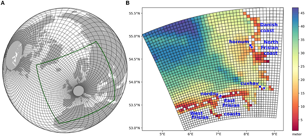
Figure 1. (A) Grid of downscaling coupled MPIOM-REMO model system. Grid lines display the grid of MPIOM. Green lines mark the EURO-CORDEX22 region of REMO, which is coupled with MPIOM. (B) Zoom of the MPIOM grid into the German Bight with grid lines and bathymetry (m) to visualize the fine horizontal resolution of MPIOM in this area. Time series at locations of Norderney (“nordny”), Cuxhaven (“cuxhav”), and Hörnum (“hornum”) will be presented in this study as representatives for the southern, central, and eastern/northern German Bight coasts. Their real positions are marked with stars, their model positions with filled circles.

For a downscaling, Mathis et al. (2018) show that the application of a regional ocean model with prescribed lateral open boundary conditions can introduce large errors to signals of changing properties. In contrast, a coupled ocean-atmosphere model system with a global ocean model focusing on the region of interest would be advantageous, because it does not need open boundary forcing data and avoids their potential problems. This holds also, if the horizontal resolution of the global ocean model is fine in the region of interest but coarse on the opposite side of the globe. Pätsch et al. (2017) compared regional model results for the North Sea with the ones of the global MPIOM and found that the global model was capable to simulate the circulation and the water mass distribution adequately, which is a proof of concept. Furthermore, the global domain of MPIOM allows for a consistent simulation of climatic signals propagating from the open Atlantic to the shelf. Therefore, the downscaling model system MPIOM-REMO is advantageous particularly for investigating climate change impacts on sea level extremes in the North Sea, driven by large-scale changes in the North Atlantic climate system.

In the following, we always refer to the simulation results of the regionalized MPIOM-REMO system if not stated otherwise.

2.2. Investigated time series, extreme values, storm surges

Observed and simulated time series have been taken as they are for validation purposes and estimation of trends. For statistical analyses, data have been detrended using the trends of the hourly time series at the corresponding stations. Detrending has been applied to all time series, not only the hourly data but also the time series of high and low water levels, even if the latter start before the hourly ones, as in case of the observed high and low water levels at Cuxhaven and Hörnum. The remaining trends in high and low water time series, which differ from each other (change of tidal range) and from trends of hourly SSH data, have not been subtracted. They are also subject of this investigation, as extreme sea levels occur only during high tidal phases.

For the investigation and comparison of the two climate states, i.e., the historical one at the end of the twentieth century and the future state at the end of the twenty-first century, the detrended results of all 30 members for the period 1970–1999 and 2070–2099 have been collected into the historic and the RCP8.5 pools, respectively. Each of these two pools contains data of 900 years representing the corresponding climate states being 100 years apart. Moreover, SSH was related to mean high water of the corresponding period by deducting it. In order to take potentially different responses along the different coastal regions of the German Bight into consideration, three locations were selected for station time series and data pools: Norderney, Cuxhaven, and Hörnum (Figure 1) as representatives for the West and East Frisian coasts, the central coast, and the Danish and North Frisian coasts, respectively.

German authorities distinguish between “regular”, heavy and extreme storm surges defined as sea surface height above the corresponding MHW plus 1.5, 2.5, 3.5 m, respectively. For the calculation of storm surge properties such as frequency, duration, and maximum height reached, storm surges were clustered to storm surge events. Storm surges, which are <60 h apart, are considered to belong to one event. Exceedance of SSH above MHW was taken from time series of tidal high and low water levels. The time of first exceedance (start time) was then interpolated from the time of the previous low water and the time of the next high water. The end time of an exceedance series was estimated correspondingly. With this, we obtained the full duration of a storm surge event. Time series of “regular” or “normal” storm surge events contain all three types of storm surge events (“normal”, heavy, and extreme), since they all are storm surges with SSH above MHW plus 1.5 m.

Our statistical analyses of extreme values like storm surge heights will also include the calculation of return levels, which are often part of engineering measures for the design of coast-protecting constructions. They express levels, which will be exceeded on average once in the associated return period (=recurrence interval, e.g., a certain level of extreme SSH above MHW will be exceeded every x years on average). This can be calculated by ranking all data of a series (like the data in a pool) in decending order and associating the reciprocal cumulative exceedance probability as return period: rp = (N+1)/r with r, N being the rank of a value and the total number of values, respectively.

Tests with block maxima other than the yearly maximum value, such as 2-, 5-, or 10-highest values per year, have shown for the observed tidal gauge time series at Cuxhaven covering more than 100 years (Supplementary Figure 1) that marked differences occur in return periods shorter than 7 years. To include these shorter time scales, we use the 10 highest values instead of only yearly maxima as extreme values of SSH in our statistical analysis. In accordance with our storm surge clustering, when collecting the 10 highest values of a year, a next highest value of the sorted series was selected only, if it was at least 60 h apart from all previous ones.

Due to the high amount of data in these 900 year pools, we are able to perform the statistical extreme value analyses with non-parametric methods. That means we do not have to select an equation to fit an analytical (theoretical) curve to the distribution of our data like the Generalized Extreme Value distribution (GEV). Such a tool is applied to extend the available amount of data and extrapolate the series, if the amount of data is not sufficient for significant statistical analyses. Using the original distribution is advantageous, since the use of fitted artificial distributions may lead to different results (Arns et al., 2013).

3. Validation of model results

Since we do not perform conventional hindcast simulations driven, e.g., with reanalysis atmospheric forcing, a validation of model results in the traditional sense is not possible. The aim is rather to produce simulation results with natural variability. Therefore, the only way of a validation is to have a look at certain statistical properties of our model results and compare these with observational data or other published climate model results.

Our simulated global mean sea surface temperature increase by about 2.3°C from 2000 to 2099 in both our global and the regionalized climate simulations (Figure 2). According to the IPCC Report AR5 (Collins et al., 2013) and AR6 (Fox-Kemper et al., 2021), this is at the lower end of the range of other climate models, which simulated the RCP8.5 and SSP5-8.5 scenarios for AR5 and AR6, respectively. From this, we expect a rather moderate effect of climate change on our simulation results compared to other models.

FIGURE 2

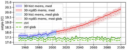
Figure 2. Ensemble range and median of global mean SST of our 30 MPIOM-REMO (solid, “med”) and MPI-ESM1.1-LR (dashed, “med glob”) ensemble simulations. Green lines: PI control simulation results.

A comparison of extreme SSH in terms of yearly maxima from tidal gauge data, PI control and ensemble simulations for Norderney, Cuxhaven, and Hörnum is presented in Figure 3. For this comparison, SSH data are not detrended but related to the respective MHW (1970–1999). The observed data do include the full mean SLR of up to 7 mm/yr in the German Bight from 1958 to 2014 (Jänicke et al., 2021), while the simulated ones do not. This is partly canceled out due to subtraction of MHW (1970–1999) from the data. The remaining SLR from 2000 to 2020 amounts to maximal 14 cm and can be neglected, because it is far below the variability (ca. 2 m) of the yearly maxima above MHW ranging from ca. 1 to 3 m. The range of all member results covers the observed time series. Moreover, most of the observed data are even within the range of ensemble mean ± standard deviation (blue shading in Figure 3). The tidal gauge data can be considered as a realization of the historical simulations fitting well into the ensemble. From this, we can conclude that the simulated extreme SSH data and their variability are well captured by the model system for the historic period.

FIGURE 3

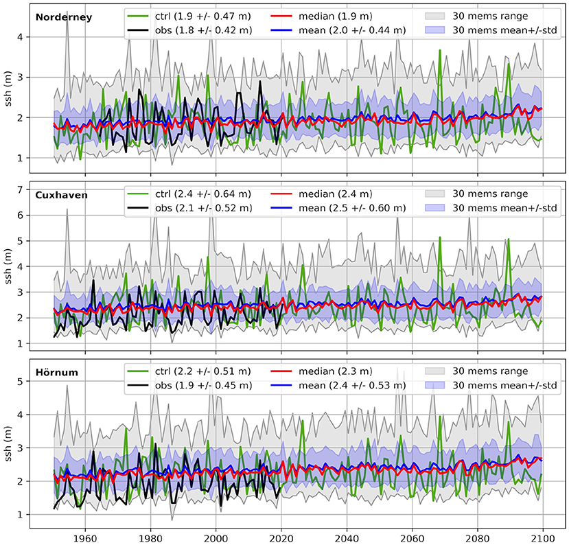
Figure 3. Extreme SSH in terms of yearly maxima above MWH (1970–1999) of the transient ensemble simulations (gray shading), ensemble mean (blue) ± ensemble standard deviation (blue shading), ensemble median (red), observed data (black), and PI control simulation (green) at Norderney, Cuxhaven, and Hörnum. For this graph, time series were not detrended. Numbers in legend: overall mean ± standard deviation, for ensemble mean: mean ± mean of standard deviation. Source of observed data: Wasserstraßen- und Schifffahrtsamt Elbe-Nordsee, location Tönning, Germany.

4. Results

4.1. Horizontal distribution of extreme SSH changes in the German Bight

Changes of extreme sea levels display quite divers patterns for the German Bight. For the southeastern North Sea, the rcp85-hist differences of the 30-, 15-, 10-, and 2-year return levels were calculated for each ensemble member. Their averages and medians are presented on horizontal maps to visualize their distribution in the German Bight region (Figure 4). Insignificant mean differences on the 95% confidence level according to the Mann–Whitney U-test are marked with dots.

FIGURE 4

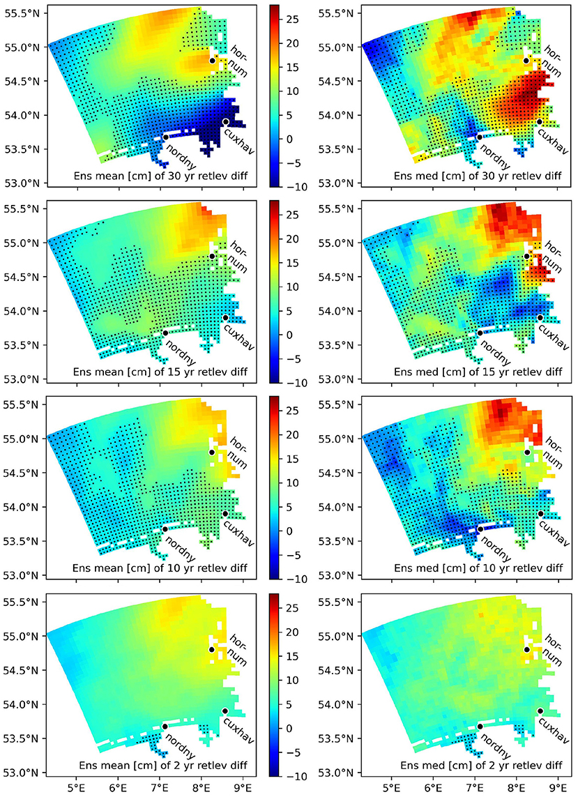
Figure 4. Ensemble mean (left) and median (right) of the rcp85-hist differences of 30-, 15-, 10-, 2-year return levels (top to bottom) in the German Bight. Statistically insignificant areas (p > 0.05) are dotted. Units correspond to a trend in cm/century.

The 30-year return levels show a significant increase near the coast only around Hörnum of 15–20 cm/century, while the 15-year return level increases significantly along the Danish coast with rates of 20–25 cm/century. A significant 10-year return level increase occurs along the entire Danish and North Frisian coasts by 13–25 cm/century with higher values in the north. The 2-year return level increases significantly nearly everywhere along the coasts of Denmark, Germany, and the Netherlands with rates of 10–17 cm/century in the north and 4–10 cm/century in the south. Also for the difference of the mean yearly maximum of each member's rcp85 and hist periods (see Supplementary Figure 2), we find significant increases everywhere in the German Bight: ensemble means and medians raise by up to 15 and 17 cm/century, respectively, in the north, by around 7.5 and 5 cm/century in the south.

Other authors found similar horizontal distributions of increasing ESL or storm surge heights. Gaslikova et al. (2013) compared their milder A1B scenario period 2071–2100 with the control period 1961–1990 and found the only statistically significant increase of storm surge heights (up to 13 cm in 110 years, 10% of control results) along the North Frisian and Danish coasts but insignificant and less increase (<8% of control results) along the East Frisian coast. Lang and Mikolajewicz (2020) found a similar distribution of significant 20- and 50-year ESL return level increases in their simulations. Estimated magnitudes of increases are also here not comparable, because they simulated another scenario (yearly 1% increase of atmospheric pCO2 from pre-industrial stage) and compare results being more than 100 years apart.

To summarize, for all significant increases of return levels, higher values are found along the Danish and North Frisian coasts, lower values along the West and East Frisian coasts. Furthermore, the ensemble median return levels always show stronger increases than the mean values. From this, we can conclude that the number of moderate storm surges will increase more than the number of extreme ones in these regions.

This high diversity regarding the change of extreme SSH in the German Bight with more significant and stronger increases along the Danish and North Frisian coasts and weaker increases along the East and West Frisian coasts is the reason to analyse data also at Norderney and Hörnum representing the aforementioned regions, and at Cuxhaven for the central German Bight coast.

4.2. Trends in extreme SSH at Norderney, Cuxhaven, and Hörnum

Observed and simulated SSH time series show trends in their yearly means and yearly maxima as well as tidal high and low water levels (see Supplementary Table 1 and Figure 3 for visual impression of yearly maxima trends). The PI control simulation displays a trend of 3 cm/century for the yearly mean SSH as well as for its tidal high and low water levels (HWL, LWL). This points to a very slight model adjustment or an imprint of natural multi-decadal variability (Lang and Mikolajewicz, 2019). The remaining 10 cm/century in the yearly mean SSH trend of the ensemble simulations at all three stations is due to climate-induced changes of water properties (density) effecting the baroclinic flow and subsequently the global dynamic circulation. Noteworthy, the simulated global mean SSH remains constant in the ensemble simulations, because MPIOM is a volume conserving ocean model.

Extreme water levels in terms of yearly maximum SSH show divers results in the ensemble simulations in the German Bight: half of the members display a significant location-dependent increase of 23–30 ± 5–7 cm/century on the 95% confidence level, which is 10–17 cm/century above the increase of SSH. This points already to a slight increase of extreme sea levels above the simulated MHW. Interestingly, the observed time series show trends (Supplementary Table 1), which basically correspond to our German Bight simulation results (Figure 4): low/no significant increase at Norderney, highest significant increase at Hörnum.

This principal distribution of trends was also found by other authors. It agrees with results of Gaslikova et al. (2013) and Lang and Mikolajewicz (2020) (as mentioned above). Sterl et al. (2009) found from climate ensemble simulations (scenario A1B corresponding to the milder RCP6.0) no storm surge height increases along the Dutch coast, which includes the West Frisian Islands. Weisse et al. (2014) review the knowledge about European ESL and summarize essentially from observations that ESL long-term trends correspond more or less to SLR. Since we simulated the stronger RCP8.5 climate scenario, it is plausible that our results show slightly higher increases along the southern and eastern German Bight coasts.

Trends in tidal high and low water levels defer from the ones in SSH for observations as well as for simulations (Supplementary Table 1). HWL increases faster and LWL similar to yearly mean SSH. Obviously, the simulated tidal range increases with time by about 0.5–1.1 cm/century (1.6–2.2 cm/century in full time series). The observational data for Cuxhaven show an order of magnitude higher tidal range trends (about 12 cm/century, corresponding to results of other authors (Jänicke et al., 2021), because our simulations do not include a global mean SLR and—with this—a potential shift of the North Atlantic Ocean and the North Sea amphidromic systems.

Supplementary Table 1 lists more details of trends in observed and simulated time series.

4.3. Return levels of storm surge heights at the three stations

The return plots of extreme SSH above the corresponding MHW (10 highest yearly values) of all 30 members for both climate states are presented in Figure 5 displaying their ranges, their median levels, their data pools, the PI control simulation results, and the observed data at Norderney, Cuxhaven, and Hörnum. Particularly for return periods less than about 4 years, the simulated data are higher than the observed data. For higher return periods, the range of simulated levels includes the observed data. This is in agreement with Figure 3, where the observed station data are also in the lower part of the simulated range of the historical extreme sea levels. The reason for this is the horizontal and particularly vertical resolution of near-coastal regions in the ocean model (see Section 6).

FIGURE 5

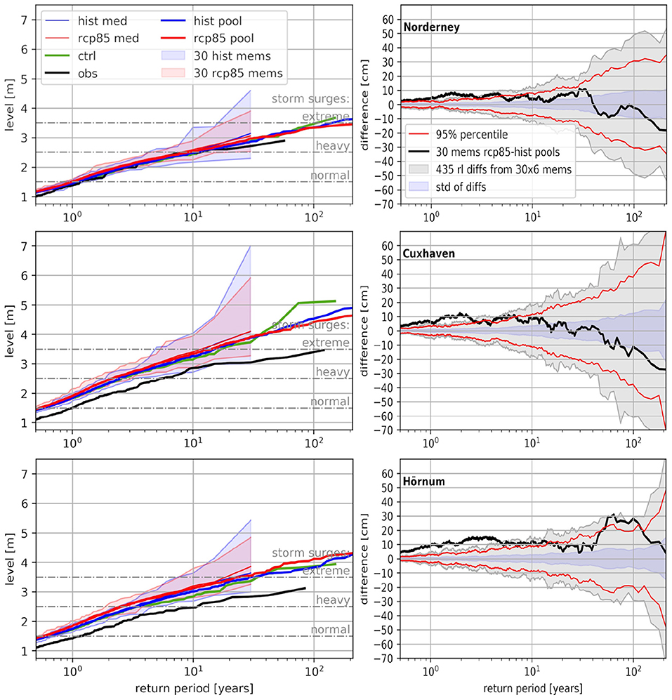
Figure 5. (Left) Return value plots for extreme ssh above MHW (yearly 10 highest) at Norderney, Cuxhaven, and Hörnum for observational data (black), PI control simulation data (green), ranges of 30 members for hist (blue shading) and rcp85 (red shading) simulation data and for the hist (red) and rcp85 (blue) pooled data. Thin red and blue lines display the median of the corresponding range. Measured data are relative to MHW (1970–1999), PI control data to MHW (1950–2099), hist member results to MHW (1970–1999), rcp85 member results to MHW (2070–2099). (Right) Difference of pooled rcp85-hist data (black), range of all possible differences of 30 pools of 6 full random members (gray shading), mean of all differences ± std (blue shading), 95 % confidence interval of all differences (red).

The difference of the pooled return levels, rcp85-hist and its significance interval on the 95% confidence level are shown in the right panels of Figure 5 (black and red lines, respectively). The significance interval between the red lines is assumed to be natural (internal) variability and therefore insignificant for change signals (calculation see below). As visible in the 2D distributions of our projected return level changes in the German Bight (Figure 4), strongest significant changes are detected along the North Frisian coast: (a) highest and most significant increase of storm surge heights are found at Hörnum, return levels of up to 13 years increase by up to 16 cm/century, return levels of 50–100 years by 25–30 cm/century; (b) storm surges are highest at Cuxhaven but not their climate-induced increase, levels with return periods below 7 years increase by up to 13 cm/century, no significant increase for longer return periods; (c) at Norderney, only up to 5-yearly return levels increase significantly by up to 8 cm/century; (d) other changes are insignificant.

When relating our results to findings of other authors, it is important to keep in mind that we infer extreme SSH above MHW. Other authors investigate the absolute extreme SSH data, which include increasing MSL probably leading to stronger climate-induced changes. Weisse et al. (2014) display in their Figure 1 observed monthly SSH maxima at Cuxhaven and estimate from their generalized extreme value distribution a 50-year return level, which increases by about 30 cm from 1920 to 2020, while their Figure 4 shows an approximate MSL increase of 18–20 cm for this period, reducing the increase of the 50-year return level to about 10 cm. Lang and Mikolajewicz (2020) found no significant increase of this return level from end of twentieth to end of twenty-first centuries—similar to our results, while Gaslikova et al. (2013) inferred an increase by about 40 cm.

In summary, maximum heights of normal and heavy storm surge events will increase significantly at all stations, most extreme ones only at Hörnum coast.

The significance interval in Figure 5 has been estimated by calculating all possible 435 return level differences of 30 data pools. Each pool consisted of the data (full 150 years) of six randomly selected members collecting 900 years of data, which were sorted in descending order to gain return levels. The absolute values of all pool differences are mirrored at the zero line to create the range of differences and to reflect that the direction of the differences does not matter. The 95% confidence interval is then the area between the positive and the negative 95th percentile of all difference amounts for each return period. Inside this confidence interval, differences are insignificant and associated with internal variability.

4.4. Overall changes of storm surge characteristics at the three stations

For a clear visualization of changes in the properties such as frequency, duration, and maximum height of clustered storm surge events, simple histogram plots at the three stations Norderney, Cuxhaven, and Hörnum are presented in Figure 6: storm surge duration vs. maximum height during an event, the number of events per year in colored shading (Section 2.2 describes our way of clustering storm surges to events). Additionally, Table 1 lists the frequency and duration data for the different storm surge types and their changes from the historical (1970–1999) to the RCP8.5 (2070–2099) pools. Table 1 gives also the proportions of heavy and extreme storm surge events among all events.

FIGURE 6

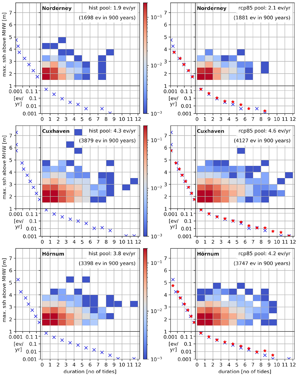
Figure 6. Clustered storm surge events: duration in numbers of tidal periods (12.425 h, 0–1 means up to 1 tidal period) vs. highest SSH (0.5 m bins) for historical and rcp85 pools (left and right) at Norderney, Cuxhaven, and Hörnum (top to bottom). Shading gives the number of events per year. Diagrams on the left and bottom of each histogram display numbers of all events per year summed over all durations and over all heights, respectively. The right diagrams show both the historical (blue crosses) and the RCP8.5 sums (red stars).

TABLE 1

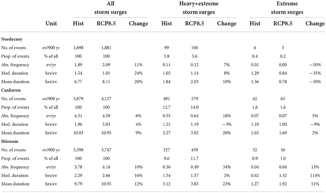
Table 1. Storm surge frequency and duration in historical and RCP8.5 pools and their changes. “prop.” means proportion, “abs.” means absolute, “med.” means median.

The total number of storm surge events increases by 10.8, 6.4, and 10.3% at the three respective stations. This originates mainly from the “normal” storm surges with MHW+1.5 m < SSH ≤ MHW+2.5 m, which are the dominant types. Heavy and extreme storm surge events show a very diverse behavior, as can be seen in Table 1. Essentially, the number of heavy events increases stronger from south to north. Occurrences of extreme events are too low at Norderney to obtain significant results, but for Cuxhaven and Hörnum, they also increase strongest in the north. Furthermore, the proportion of heavy events increases, while the one of extreme events rather decreases (except for Hörnum) during the 100 years from our historical to RCP8.5 periods.

The mean duration of storm surge events clearly increases for all types and at all stations (Figure 6, Table 1). While the historical period shows hardly storm surge events longer than 9 tidal periods, they might last a tidal cycle longer a 100 years later. However, the maximum duration does not change. The large difference to the median duration—the mean is about the five-fold median—is due to the fact that shorter storm surges occur much more often than longer ones. The median duration of all events increases by 4-5 percentage points more than the mean at Norderney and Hörnum (Table 1). Obviously, the frequency of shorter lasting events increases more than the longer ones at the two stations. In contrast, the Cuxhaven median duration increases by ca. 5 points less than the mean: frequency of longer storm surge events increases stronger than for shorter ones.

In agreement to our previous findings, Figure 6 also illustrates that there is no change of the overall maximum SSH achieved during storm events in our simulated data. This means that the extreme SSH values reached during storm surge events increase with a similar rate as the MHW, which raises slightly faster than the mean sea level. Weisse et al. (2014) concluded also from their investigation similar long-term trends of ESL and MSL. For the other content of this section, the authors could not find corresponding published study results to be compared with.

4.5. Seasonal changes of storm surge characteristics at the three stations

The seasonal changes of absolute frequency and mean and maximum duration of storm surge events are presented for all three known stations in Figure 7 for the hist and the rcp85 pools. Supplementary Figure 3 shows additionally the observational and control simulation data for these parameters plus the relative frequency and the median duration.

FIGURE 7

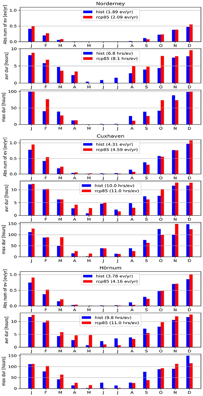
Figure 7. Clustered storm surge events (all types) for each month of a year at Norderney, Cuxhaven, Hörnum. (First panels) absolute frequencies; (middle and lower panels) average and maximum duration. Numbers in legends are calculated over all events in the corresponding pools.

For all storm surge events, the seasonal distribution shows a clear change signal regarding absolute frequency (upper panels in Figure 7) as well as relative frequency (second panel in Supplementary Figure 3) of storm surge events. The absolute frequency increases overall by the end of this century but only in December to April, while it decreases in August to November at all stations. This shift of the storm surge season has been found by Lang and Mikolajewicz (2020) as well in their 1% scenario simulations.

The average duration of events (middle panels in Figure 7) at Norderney and Hörnum increases during the storm season October to February/March. In the central German Bight, at Cuxhaven, the mean duration increases in the last 3 months of a year, while the absolute number of events decreases in October and November. So, during these months, longer events increase more than shorter ones.

The maximum duration of storm surge events (lower panel in Figure 7) does not show a clear seasonal change between the two climate periods. Even its overall maximum does not change due to RCP8.5 climate change until the end of this century. Although these distributions originate from single (random) events, this result is in line with the general trend toward more frequent and partly longer lasting events with slightly higher maximum SSH in the future but no overall increase.

For heavy+extreme storm surge events (not shown), there is no clear seasonal change visible in the data. During May, June, and July, no historical and no RCP8.5 heavy storm surge events occur neither in observations nor in the model simulations. Extreme storm surge events are too seldom to obtain significant statements. While there are no extreme storm surges during April to September in the historical and control simulations at all stations, the rcp85 pool shows some short events in April and September.

5. The main cause of storm surge changes: Wind

In the previous section, we described changes in storm surge characteristics found in our simulation results. We detected an increase in frequency, more in the first quarter of a year than in the last one, and an increase in duration of clustered storm surge events. In addition, our analyses showed no increase in overall severity (maximum height) of storm surges but weak rises along the West and East Frisian and moderate rises along the North Frisian and Danish coasts.

There are several phenomena, which can modify (and increase) storm surges in the German Bight. The most important driver is a wind with sufficient speed or speed and duration from westerly directions (Dangendorf et al., 2014). External surges, which are generated by North Atlantic storm events or by an altered North Atlantic circulation with increased sea levels in the east, can travel into the North Sea, propagate like a tidal wave to the German Bight and potentially amplify storm surges (Müller-Navarra and Giese, 1999; Ganske et al., 2018; Grabemann et al., 2020). Moreover, low pressure systems over the deep regions northeast of Scotland can induce waves traveling similarly to the German Bight and increase high water levels (Bruss et al., 2010). Also, extremely low air pressure above the area of interest could lead to a further lift of the sea surface (inverse barometric effect).

In this article, we focus on the main factor wind speed and direction and their climate-induced changes. Up to 90% of the observed MSL variability at Cuxhaven can be explained with the zonal wind stress (Dangendorf et al., 2013). Since our simulated sea level variability agrees well with the observed at all three stations (Figure 3), we can assume that our wind simulation results are also reasonably well-reflecting the natural wind variability.

After collecting the wind data in a similar way as the SSH data for the storm surge analyses obtaining again 900 years data pools, we further collect the wind speed data in 10° direction bins. The distribution of certain statistical parameters of wind speed as a function of these wind direction bins is presented in Figure 8. We find slight increases in speed for the 1-, 5-, 30-, and 50-year return levels especially for southwesterly to westerly wind directions. Moreover, the frequency of wind speeds above 20 m/s (almost 9 Bft) clearly increases for directions of 225–300° with the largest change at around 270°. This would be sufficiently strong to generate storm surges in the German Bight (Ganske et al., 2018). Thus, the detected increases concern rather westerly and southwesterly directions, which agrees well with our results of stronger increasing storm surge activities in the north. A frequency increase of southwesterly to westerly strong winds was also detected by Gaslikova et al. (2013) in their A1B scenario simulations, while Lang and Mikolajewicz (2020) inferred rather more frequent wind maxima coming from 250 to 300°.

FIGURE 8

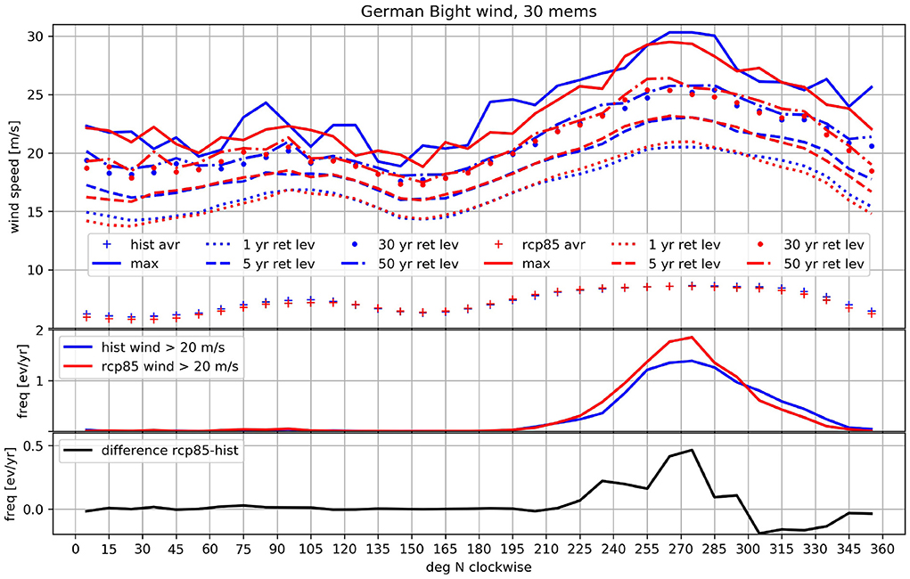
Figure 8. Wind speed, direction, and frequency for the marine German Bight region from hist and rcp85 pools (blue and red colors, respectively). Wind data have been collected in 10° bins of the wind direction. (Upper) Average and maximum wind speed as well as 5-, 30-, and 50-year return levels in the bins. (Middle) Frequency in events per year for wind speeds above 20 m/s. (Lower) rcp85-hist difference of frequencies in (Middle).

The frequency data in Figure 8 include all data exceeding 20 m/s without clustering. Higher values of this frequency lead to both higher frequencies of resulting storm surge events as well as to higher duration of storm events.

The monthly distribution of wind speed, direction, and frequency in direction bins (Supplementary Figure 4 and Supplementary Table 2) displays for the rcp85 pool clearly higher frequencies of wind directions around 270° during the “kernel storm season” from October to March with strongest increases in January and February. The average velocity of these winds hardly changes, which is the reason, why we hardly detect changes in the maximum surge levels or in extreme storm surge activities at all.

Overall, our simulation results show a clear increase of frequency and duration of storm surges in the entire German Bight but an increase in maximum height reached during storm surges only in the northern German Bight and along the Danish west coast.

6. Discussion

Müller-Navarra and Giese (1999) calculated storm surge effective wind directions for the German Bight (Wilhelmshaven) to be between westerly and northerly. Ganske et al. (2018) list the newly defined parameter “effective wind”, which was calculated following Müller-Navarra and Giese (1999), for the German Bight to be between 295° at Husum (northern German Bight coast) and 315° at Borkum (southern German Bight coast). The “effective wind” is defined as the projection of the 10 m horizontal wind to the direction with the most severe impact on the coastal water level (highest wind surge). Gönnert (2003) investigated storm surge and wind time series and found the “critical wind direction” for “normal” to heavy storm surges to be 230–360°, for extreme storm surges 280–310°. Jensen et al. (2006) mention a wind direction of 247.5–337.5° as a condition for potential storm surges in the inner German Bight. Obviously, there is a range of wind directions responsible for storm surges in the German Bight with southwesterly directions to be effective for the northern German Bight coasts and northwesterly directions effecting rather the southern parts of the German Bight.

In our analyses, we found an increasing frequency of southwesterly to westerly strong winds with a weak increase of wind speed. According to Müller-Navarra and Giese (1999) and Gerber et al. (2016), these directions would rather effect the North Frisian and Danish coasts, which is well supported by our findings. Northwesterly strong winds, which would increase the number or heights of storm surges along the East and West Frisian coasts, occur hardly with higher frequency or strength. The result of all this is the pronounced increase of return levels along the North Frisian and Danish coasts and a weak or no increase along the West and East Frisian coasts, as visible in Figure 4. However, the climate change impact induced in our model simulations by the RCP8.5 emission scenario is not sufficient to create overall higher storm surge levels in terms of SSH above MHW than nowadays.

We have to keep in mind, that a SLR itself would already increase the SSH above MHW in the German Bight (tidal high water levels would increase more than the sea level itself). Jänicke et al. (2021) have shown this already for North Sea stations for the past. The reason is a physical one: a reduced damping (Idier et al., 2017). The bottom friction effect is reduced in deeper water allowing the tidal wave to be higher. This would subsequently result in higher potential sea levels during storm surges. Arns et al. (2015) estimated from model investigations that a MSL raise of 54 cm would lead to an increase of storm surge heights of up to 15 cm around the North Frisian Islands, which is, however, location-dependent due to non-linear effects. Additionally, a stronger stratification due to more heating from the atmosphere would have this effect as well, which is explained in more detail by Li et al. (2021).

Furthermore, there are certain limitations of our downscaling ocean model setting due to the horizontal resolution and particularly the surface layer thickness of 16 m. This prevents the consideration of shallow coastal areas, especially the Wadden Sea, which has a damping effect not only for tides but also for the propagation of storm surges (see paragraph above). Additionally, the shallow but large Wadden Sea and large estuaries like the one of the Elbe River act as a temporary buffer for water piled up by the wind, which can reduce the extreme sea level, because the water masses are distributed over a larger area. However, this is valid for all simulations and the entire period to the same extent and is canceled out when comparing different temporal segments of the entire period.

The influence of external storm surges was not investigated here but is subject for further data analyses. The fact of more frequent winds from the west may be accompanied by more external surges from the North Atlantic, which would have an influence on German Bight storm surges. Our results suggest indirectly that the external surges play a minor role, because our simulated storm surges did not increase in height. On the other hand, they may have directly increased the frequency. This is subject to further analyses.

Wind waves have also not been considered in our numerical simulations, which could be done by additionally employing a wind wave model. Idier et al. (2019) mention that waves can increase storm surges by a few up to tens of centimeters. Mean sea level rise, waves and external storm surges could potentially increase the maximum sea level reached during storm surge events.

With our approach, model uncertainties have not been considered, because we used only one model system for all simulations. However, we mentioned in the validation section that our general model results such as global mean SST are within the range of other model simulations published by the IPCC (Collins et al., 2013; Fox-Kemper et al., 2021).

As published by other authors already, weather conditions may become more persistent in future with decreasing temperature differences between the poles and low latitudes, which is, however, still under debate (Kornhuber and Tamarin-Brodsky, 2021). This theory would be supported by our findings of longer lasting storms followed by correspondingly longer lasting storm surge events in the future.

7. Summary and conclusions

For the investigation of climate-induced changes in maximum height, frequency, and duration of storm surges in the German Bight, the regionalized climate model system MPIOM-REMO was applied to create a simulation ensemble of thirty members for the historical period 1950–2005 and the continuation until 2099 under the RCP8.5 scenario. A pre-industrial (PI) control simulation was also run for the entire period. The model system consisted of the global ocean circulation model MPIOM with a fine horizontal resolution in the North Sea region, which was coupled with the regional atmospheric circulation model REMO over the EURO-CORDEX region. Outside the domain of REMO, the system was forced with simulation results of the previously performed global climate simulation ensemble with MPI-ESM1.1-LR for the same period on the base of thirty different initial states in 1950. Results of all regionalized members of the period 1970–1999 and 2070–2099 have been collected into the historical and the rcp85 pools, respectively, adding up 900 years of model results of the corresponding climate state.

Due to an adaptation of the global circulation to the RCP8.5-induced climate change, the mean ensemble German Bight SSH trend amounts to about 13 ± 1 cm/century (PI control: 3 cm/century). Storm surges were defined according to the German authorities as occurrences with SSH above mean tidal high water (MHW) plus 1.5, 2.5, 3.5 m for “regular”, heavy, and extreme storm surges, respectively, and clustered to storm surge events if <60 h apart. MHW raised with a slightly higher rate than the mean SSH of about 14 ± 1 cm/century, while mean tidal low water increased with a smaller rate indicating a tidal range increase.

Our ensemble simulations clearly show an increase in frequency and duration of storm surge events. The change of maximum height of events shows a divers pattern in the German Bight with significant high increases along the North Frisian and Danish coasts and low increases along the West and East Frisian coasts: At Hörnum (North Frisian coast), return levels of up to 13 years increase by up to 16 cm/century, return levels of 50–100 years by 25–30 cm/century; at Cuxhaven (central German Bight coast), up to 7-year return levels increase by up to 13 cm/century, further significant increases are not detected; at Norderney (East Frisian coast), only levels below 5-year return period increase significantly by up to 8 cm/century. Higher storm surge return levels do not increase relative to the corresponding MHW. Thus, extreme storm surge events show hardly any response to the climate change induced by the RCP8.5 emission scenario. A shift of seasonality is obtained in the simulated data from the last to the first quarter of a year.

The detected changes of storm surge characteristics are associated with changes in the wind fields showing a pronounced increase of occurrence of strong southwesterly to westerly winds with only a slight increase of wind speed during storm surge events. These wind directions are able to produce storm surges along the North Frisian and Danish coasts. Consequently, pronounced significant increases in return levels are detectable along these coasts.

Owing to the large number of our ensemble simulations, we were—for the first time—able to show in an explicit and non-parametric way that the climate change signal of extreme storm surges in the German Bight is strongly blurred by high natural variability, even in a strong global warming scenario. Only for the Danish and North Frisian coasts, the climate change due to this scenario was strong enough to significantly increase storm surge return levels of more than about 7 years.

Data availability statement

The datasets presented in this study can be found in online repositories. The names of the repository/repositories and accession number(s) can be found at: doi: 10.26050/WDCC/ECCES_MPIOM-REMO.

Author contributions

BM created the database, performed the analysis, and wrote the first draft of the manuscript. UM contributed with suggestions of analyses methods to be applied. MM and TP contributed to conception and design of the study. All authors contributed to manuscript revision, read, and approved the submitted version.

Funding

This research was performed within the project ECCES: Effects of climate change on extreme sea levels in the North Sea under realistic consideration of external surges and atmosphere-ocean feedback mechanisms, which was part of ClimXtreme, a German research network on climate change and extreme events. ECCES was funded by the German Federal Ministry of Education and Research (BMBF) under grant number 01LP1901B. MM was funded by Germany's Excellence Strategy EXC 2037 CLICCS—Climate, Climatic Change, and Society with project No. 390683824.

Acknowledgments

We would like to thank the DKRZ (Deutsches Klimarechenzentrum, German Climate Computing Center) and their great support. Their computational resources were made available through funding support from the German Federal Ministry of Education and Research (BMBF). We would also like to thank Veit-Hinnerk Bayer of the Wasserstraßen- und Schifffahrtsamt Elbe-Nordsee as well as Michael Nicklau of Wasserstraßen- und Schifffahrtsamt Ems-Nordsee for providing tidal gauge data and helpful information about these observations.

Conflict of interest

The authors declare that the research was conducted in the absence of any commercial or financial relationships that could be construed as a potential conflict of interest.

Publisher's note

All claims expressed in this article are solely those of the authors and do not necessarily represent those of their affiliated organizations, or those of the publisher, the editors and the reviewers. Any product that may be evaluated in this article, or claim that may be made by its manufacturer, is not guaranteed or endorsed by the publisher.

Supplementary material

The Supplementary Material for this article can be found online at: https://www.frontiersin.org/articles/10.3389/fclim.2022.992119/full#supplementary-material

References

Arns, A., Wahl, T., Dangendorf, S., and Jensen, J. (2015). The impact of sea level rise on storm surge water levels in the northern part of the German bight. Coast. Eng. 96, 118–131. doi: 10.1016/j.coastaleng.2014.12.002

CrossRef Full Text | Google Scholar

Arns, A., Wahl, T., Haigh, I., Jensen, J., and Pattiaratchi, C. (2013). Estimating extreme water level probabilities: a comparison of the direct methods and recommendations for best practise. Coast. Eng. 81, 51–66. doi: 10.1016/j.coastaleng.2013.07.003

CrossRef Full Text | Google Scholar

Arns, A., Wahl, T., Wolff, C., Vafeidis, A., Haigh, I., Woodworth, P., et al. (2020). Non-linear interaction modulates global extreme sea levels, coastal flood exposure, and impacts. Nat. Commun. 11:1918. doi: 10.1038/s41467-020-15752-5

PubMed Abstract | CrossRef Full Text | Google Scholar

Bruss, G., Gönnert, G., and Mayerle, R. (2010). Extreme scenarios at the german north sea coast a numerical model study. Coast. Eng. Proc. 1. doi: 10.9753/icce.v32.currents.26

CrossRef Full Text | Google Scholar

Chang, E. K., and Fu, Y. (2002). Interdecadal variations in northern hemisphere winter storm track intensity. J. Clim. 15, 642–658. doi: 10.1175/1520-0442(2002)015<0642:IVINHW>2.0.CO;2

CrossRef Full Text | Google Scholar

Collins, M., Knutti, R., Arblaster, J., Dufresne, J.-L., Fichefet, T., Friedlingstein, P., et al. (2013). Long-term Climate Change: Projections, Commitments and Irreversibility. Cambridge: Cambridge University Press.

Google Scholar

Dangendorf, S., Calafat, F. M., Arns, A., Wahl, T., Haigh, I. D., and Jensen, J. (2014). Mean sea level variability in the north sea: processes and implications. J. Geophys. Res. 119, 6820–6841. doi: 10.1002/2014JC009901

CrossRef Full Text | Google Scholar

Dangendorf, S., Mudersbach, C., Wahl, T., and Jensen, J. (2013). Characteristics of intra-, inter-annual and decadal sea-level variability and the role of meteorological forcing: the long record of Cuxhaven. Ocean Dyn. 63, 209–224. doi: 10.1007/s10236-013-0598-0

CrossRef Full Text | Google Scholar

Elizalde, A., Groeger, M., Mathis, M., Mikolajewicz, U., Bülow, K., Hüttl-Kabus, S., et al. (2014). Mpiom-remo a coupled regional model for the north sea. KLIWAS Schrift. 58, 17. doi: 10.5675/Kliwas_58/2014_MPIOM-REMO

CrossRef Full Text | Google Scholar

Fox-Kemper, B., Hewitt, H., Xiao, C., Adalgeirsdóttir, G., Drijfhout, S., Edwards, T., et al. (2021). Ocean, Cryosphere and Sea Level Change. Cambridge; New York, NY: Cambridge University Press, 1211–1362.

Google Scholar

Ganske, A., Fery, N., Gaslikova, L., Grabemann, I., Weisse, R., and Tinz, B. (2018). Identification of extreme storm surges with high-impact potential along the German North Sea coastline. Ocean Dyn. 68, 1371–1382. doi: 10.1007/s10236-018-1190-4

CrossRef Full Text | Google Scholar

Gaslikova, L., Grabemann, I., and Groll, N. (2013). Changes in north sea storm surge conditions for four transient future climate realizations. Nat. Hazards 66, 1501–1518. doi: 10.1007/s11069-012-0279-1

CrossRef Full Text | Google Scholar

Gerber, M., Ganske, A., Müller-Navarra, S., and Rosenhagen, G. (2016). Categorisation of meteorological conditions for storm tide episodes in the german bight. Meteorol. Zeitsch. 25, 447–462. doi: 10.1127/metz/2016/0660

CrossRef Full Text | Google Scholar

Giorgetta, M. A., Jungclaus, J., Reick, C. H., Legutke, S., Bader, J., Bottinger, M., et al. (2013). Climate and carbon cycle changes from 1850 to 2100 in mpi-esm simulations for the coupled model intercomparison project phase 5. J. Adv. Model. Earth Syst. 5, 572–597. doi: 10.1002/jame.20038

CrossRef Full Text | Google Scholar

Gönnert, G. (2003). Sturmfluten und windstau in der Deutschen Bucht - Charakter, veränderungen und maximalwerte im 20. Jahrhundert. Die Küste 67, 185–365. Available online at: https://hdl.handle.net/20.500.11970/101500

Google Scholar

Grabemann, I., Gaslikova, L., Brodhagen, T., and Rudolph, E. (2020). Extreme storm tides in the german bight (North sea) and their potential for amplification. Nat. Hazards Earth Syst. Sci. 20, 1985–2000. doi: 10.5194/nhess-20-1985-2020

CrossRef Full Text | Google Scholar

Idier, D., Bertin, X., Thompson, P., and Pickering, M. D. (2019). Interactions between mean sea level, tide, surge, waves and flooding: mechanisms and contributions to sea level variations at the coast. Surveys Geophys. 40, 1603–1630. doi: 10.1007/s10712-019-09549-5

CrossRef Full Text | Google Scholar

Idier, D., Cois Paris, F., Cozannet, G. L., Boulahya, F., and Dumas, F. (2017). Sea-level rise impacts on the tides of the european shelf. Contin. Shelf Res. 137, 56–71. doi: 10.1016/j.csr.2017.01.007

CrossRef Full Text | Google Scholar

Jänicke, L., Ebener, A., Dangendorf, S., Arns, A., Schindelegger, M., Niehüser, S., et al. (2021). Assessment of tidal range changes in the North sea from 1958 to 2014. J. Geophys. Res. 126:e2020JC016456. doi: 10.1029/2020JC016456

PubMed Abstract | CrossRef Full Text | Google Scholar

Jensen, J., Mudersbach, C., Müller-Navarra, S., H.; Bork, I., Koziar, C., and Renner, V. (2006). Modellgestützte untersuchungen zu sturmfluten mit sehr geringen eintrittswahrscheinlichkeiten an der deutschen Nordseeküste. Die Küste 71, 123–167. Available online at: https://hdl.handle.net/20.500.11970/101559

Google Scholar

Kornhuber, K., and Tamarin-Brodsky, T. (2021). Future changes in northern hemisphere summer weather persistence linked to projected arctic warming. Geophys. Res. Lett. 48:e2020GL091603. doi: 10.1029/2020GL091603

CrossRef Full Text | Google Scholar

Lang, A., and Mikolajewicz, U. (2019). The long-term variability of extreme sea levels in the german bight. Ocean Sci. 15, 651–668. [10.5194/os-15-651-2019]10.5194/os-15-651-2019

Google Scholar

Lang, A., and Mikolajewicz, U. (2020). Rising extreme sea levels in the German Bight under enhanced CO₂ levels: a regionalized large ensemble approach for the North Sea. Clim. Dyn. 55, 1829–1842. doi: 10.1007/s00382-020-05357-5

CrossRef Full Text | Google Scholar

Li, W., Mayer, B., and Pohlmann, T. (2021). The influence of baroclinity on tidal ranges in the north sea. Estuar. Coast. Shelf Sci. 250:107126. doi: 10.1016/j.ecss.2020.107126

CrossRef Full Text | Google Scholar

Marcos, M., and Woodworth, P. L. (2018). Changes in extreme sea levels. CLIVAR Exchanges 20–24. Available online at: https://nora.nerc.ac.uk/id/eprint/519546/1/Variations-Exhanges-Winter2018.pdf#page=21

Google Scholar

Mathis, M., Elizalde, A., and Mikolajewicz, U. (2018). Which complexity of regional climate system models is essential for downscaling anthropogenic climate change in the Northwest European Shelf? Clim. Dyn. 50, 2637–2659. doi: 10.1007/s00382-017-3761-3

CrossRef Full Text | Google Scholar

Mathis, M., Elizalde, A., and Mikolajewicz, U. (2019). The future regime of atlantic nutrient supply to the northwest European shelf. J. Mar. Syst. 189, 98–115. doi: 10.1016/j.jmarsys.2018.10.002

CrossRef Full Text | Google Scholar

Mathis, M., and Mikolajewicz, U. (2020). The impact of meltwater discharge from the greenland ice sheet on the atlantic nutrient supply to the northwest European shelf. Ocean Sci. 16, 167–193. doi: 10.5194/os-16-167-2020

CrossRef Full Text | Google Scholar

Mikolajewicz, U., Sein, D. V., Jacob, D., Koenigk, T., Podzun, R., and Semmler, T. (2005). Simulating Arctic sea ice variability with a coupled regional atmosphere-ocean-sea ice model. Meteorol. Zeitsch. 14, 793–800. doi: 10.1127/0941-2948/2005/0083

CrossRef Full Text | Google Scholar

Müller-Navarra, S. H., and Giese, H. (1999). Improvements of an empirical model to forecast wind surge in the German Bight. Deutsch. Hydrogr. Zeitsch. 51, 385–405. doi: 10.1007/BF02764162

CrossRef Full Text | Google Scholar

Pätsch, J., Burchard, H., Dieterich, C., Gräwe, U., Gröger, M., Mathis, M., et al. (2017). An evaluation of the north sea circulation in global and regional models relevant for ecosystem simulations. Ocean Model. 116, 70–95. doi: 10.1016/j.ocemod.2017.06.005

CrossRef Full Text | Google Scholar

Rasquin, C., Seiffert, R., Wachler, B., and Winkel, N. (2020). The significance of coastal bathymetry representation for modelling the tidal response to mean sea level rise in the german bight. Ocean Sci. 16, 31–44. doi: 10.5194/os-16-31-2020

CrossRef Full Text | Google Scholar

Rogers, J. C. (1997). North atlantic storm track variability and its association to the north atlantic oscillation and climate variability of northern europe. J. Clim. 10, 1635–1647.

Google Scholar

Sein, D. V., Mikolajewicz, U., Gröger, M., Fast, I., Cabos, W., Pinto, J. G., et al. (2015). Regionally coupled atmosphere-ocean-sea ice-marine biogeochemistry model rom: 1. Description and validation. J. Adv. Model. Earth Syst. 7, 268–304. doi: 10.1002/2014MS000357

CrossRef Full Text | Google Scholar

Sterl, A., van den Brink, H., de Vries, H., Haarsma, R., and van Meijgaard, E. (2009). An ensemble study of extreme storm surge related water levels in the north sea in a changing climate. Ocean Sci. 5, 369–378. doi: 10.5194/os-5-369-2009

CrossRef Full Text | Google Scholar

Thomas, M., Sündermann, J., and Maier-Reimer, E. (2001). Consideration of ocean tides in an OGCM and impacts on subseasonal to decadal polar motion excitation. Geophys. Res. Lett. 28, 2457–2460. doi: 10.1029/2000GL012234

CrossRef Full Text | Google Scholar

Valcke, S. (2013). The oasis3 coupler: a European climate modelling community software. Geosci. Model Dev. 6, 373–388. doi: 10.5194/gmd-6-373-2013

CrossRef Full Text | Google Scholar

Weisse, R., Bellafiore, D., Menéndez, M., Méndez, F., Nicholls, R. J., Umgiesser, G., et al. (2014). Changing extreme sea levels along european coasts. Coast. Eng. 87, 4–14. doi: 10.1016/j.coastaleng.2013.10.017

CrossRef Full Text | Google Scholar

Weisse, R., and von Storch, H. (2009). Marine Climate and Climate Change. Storms, Wind Waves and Storm Surges, 1st Edn. Berlin; Heidelberg: Springer.

Google Scholar

Woth, K., Weisse, R., and Von Storch, H. (2006). Climate change and north sea storm surge extremes: an ensemble study of storm surge extremes expected in a changed climate projected by four different regional climate models. Ocean Dyn. 56, 3–15. doi: 10.1007/s10236-005-0024-3

CrossRef Full Text | Google Scholar