Forced changes in El Niño–Southern Oscillation due to global warming and the associated uncertainties in ACCESS-ESM1.5 large ensembles

Understanding the forced response of El Niño–Southern Oscillation (ENSO) to future global warming (GW) is important for reliable climate projections; however, many important aspects of this response are yet to be fully understood. Here, we use two large ensembles of CMIP6 historical and SSP3-7.0 experiments (each with 40 ensemble members), performed with ACCESS-ESM1.5, to investigate the combined greenhouse gas (GHG) and aerosol forced changes in selected ENSO properties. We document the forced changes in ENSO's amplitude, power spectrum, skewness, and feedbacks and quantify the internal variability associated with these forced changes. There is a modest but statistically significant GW-induced increase in the ensemble-mean ENSO amplitude and a sizable ensemble variation (due to internal variability) with both increases (in 80% of the members) and decreases. To understand the mechanism of this variation, we examine the role of changes in the mean state and atmosphere-ocean coupling processes in the Pacific. We find that the ensemble variation of GW-induced ENSO amplitude change is most sensitive to the zonal wind forcing change. A change in the zonal gradient of mean sea surface temperatures (SSTs) also plays an important role in the ENSO amplitude change, with the changes in the atmospheric Bjerknes feedback and thermocline feedback playing a minor role. The implications and some caveats of these findings are discussed.

Introduction

El Niño–Southern Oscillation (ENSO) is the dominant mode of interannual climate variability, which impacts global weather through teleconnections. It is important to understand its dynamical responses to the historical and future climate changes, in order to provide skillful predictions of ENSO under the present climate and reliable projections under a possible future warming climate. Observational data have played a central role in increasing our understanding of historical ENSO variability (Bjerknes, 1969; Rasmusson and Carpenter, 1982; Wallace et al., 1998). Models have also played a critical role in this understanding by interpreting observational data and providing a tool to examine different aspects of ENSO dynamics by experimentations (Gill and Rasmusson, 1983; Zebiak and Cane, 1987; Battisti and Hirst, 1989; Jin, 1997). Subsequently, models of intermediate complexity have been successfully used in routine predictions of ENSO variability at seasonal-to-interannual timescales. At the same time, global atmosphere-ocean coupled models with comprehensive physical parametrizations (hereafter, CGCMs) and earth system models (ESMs) with the addition of biogeochemical processes have been developed for wider climate and earth system applications. Different generations of these models have been used in successive Coupled Model Intercomparison Projects (CMIPs), under which numerical simulations were performed with standardized forcing datasets for pre-industrial, historical and possible future climate conditions (Taylor et al., 2012; Eyring et al., 2016). Among other things, these climate simulations have provided an unprecedented opportunity to study climate variability associated with historical ENSO events and their changes under possible future pathways of anthropogenic GHG and aerosol emissions.

A significant number of past studies have sought to understand the effects of GHG induced global warming (GW) on ENSO variability using multi-model simulations from various CMIP archives (Philip and van Oldenborgh, 2006; Collins et al., 2010; Chen et al., 2015, 2017; Ham and Kug, 2016; Rashid et al., 2016; Ying et al., 2019; Fredriksen et al., 2020; Cai et al., 2021). Many of these studies showed a small forced (i.e., ensemble-averaged) response of ENSO to GW (but with a large inter-model variation), while others reported a strong forced ENSO response, often using a subset of models chosen based on some criteria. However, the latest, CMIP6 models show a somewhat stronger ensemble-mean increase in ENSO variability than the CMIP5 models do (Fredriksen et al., 2020; Grose et al., 2020; Cai et al., 2022). Contrasting results of weakened ENSO variability in equilibrated GW simulations have also been published (e.g., Callahan et al., 2021). While much has been learned from such multi-model studies, an obstacle to reconciling the contrasting results has been the structural differences between different models used in these studies. The structural difference arises from differences in the model formulation, numerics, and physical parametrizations of the participating models, among other things. With the recent advances in high performance computing, many modeling centers have now performed large ensembles (LEs) of simulations using single models, with typically more than 30 ensemble members per experiment. The LEs use the same set of forcing (for the same experiment) but different initial conditions and thus provide an opportunity to remove the effect of structural differences from model analysis results including ENSO analysis (Zheng et al., 2018; Deser et al., 2020; Ng et al., 2021; Hyun et al., 2022). However, a downside of such single-model LEs is that the analysis results may be affected by any systematic biases of the model, which could otherwise be greatly reduced using a large enough multi-model ensemble. Therefore, single-model LEs are not a replacement, rather they are complementary to multi-model ensembles.

In this study, we investigate the response of ENSO to GW using two sets of single-model LE simulations performed with the Australian Community Climate and Earth System Simulator version 1.5 (ACCESS-ESM1.5) (Ziehn et al., 2020). The experiments used are the CMIP6 historical and SSP3-7.0 experiments. We choose the SSP3-7.0 experiment over other ScenarioMIP experiments, as this was recommended for performing large ensemble simulations and studying the potential changes in internal variability mode, such as ENSO, over a substantial range of global average radiative forcing and temperature change (Eyring et al., 2016; O'Neill et al., 2016). Some previous studies looked at ENSO responses to GW using single-model LEs for CMIP5 experiments (Maher et al., 2018; Zheng et al., 2018; Ng et al., 2021; Hyun et al., 2022). They found small increases or decreases in ensemble-mean (i.e., forced) ENSO amplitude with large ensemble variations (or, inter-member uncertainties); Maher et al. (2018) and Ng et al. (2021) also found different ENSO responses in two different models. Hyun et al. (2022) suggest that an inverse relationship between the intensity of present-day internal variability and future ENSO amplitude change is the cause of ensemble variations they found in two large ensembles. They, however, did not offer any physical mechanism for such an inverse relationship. Here, we find a small but statistically significant forced change in ENSO amplitude in ACCESS-ESM1.5 LE, with a wide variation among the ensemble members. In addition to this forced ENSO response and the associated uncertainties, we investigate the role of the main ENSO processes in the ensemble variation of the ENSO amplitude change. In particular, we examine the impacts of GW-induced changes in ENSO forcing, ENSO feedbacks and the zonal gradient of tropical Pacific mean SSTs on ensemble variations of ENSO amplitude change. To our knowledge, this is the first attempt to examine the relation between the ENSO amplitude and process changes in single-model LEs.

This article is organized as follows. First, we describe the observational data, ACCESS-ESM1.5 LE simulations for the historical and SSP3-7.0 experiments, and the analysis method. The changes in the tropical Pacific mean-state SST between two experiments are then described. After this, we discuss the changes of selected ENSO properties under GW; this is followed by a discussion of the relative contributions of the mean-state SST and different ENSO processes to ENSO amplitude changes. Finally, a summary and discussion of the results are provided.

Observational and reanalysis data, ACCESS-ESM1.5 large ensembles, and analysis method

The SST data for 1870–2014 from the HadISST dataset (Rayner et al., 2003), zonal wind stress (ZWS) (1958–2014) from ERA interim and ERA5 reanalyses (Dee et al., 2011; Hersbach et al., 2020), and the thermocline depth (THD) (1958–2014) calculated from the ORAS4 ocean temperature reanalysis (Balmaseda et al., 2013) were used to compare with the analysis results of ACCESS-ESM1.5 historical LE simulations. The ACCESS-ESM1.5 historical and SSP3-7.0 LE simulations, each with 40 members, cover the 1850–2014 and 2015–2100 periods, respectively. The same CMIP6 historical and future scenario forcing data were used as boundary conditions for all simulations of the respective experiment, with different ensemble members starting from different initial conditions. The latter were taken from the ACCESS-ESM1.5 pre-industrial control simulation at 20-year intervals. The details of the ACCESS-ESM1.5 model and its experiment designs for CMIP6 have been described in Ziehn et al. (2020). An overview of all the ACCESS simulations for CMIP6, the preparation of forcing datasets and some climate and biogeochemical results are presented in Mackallah et al. (2022). Rashid et al. (2022) discuss the simulation of historical climate variability (including ENSO) and change in a subset of the ACCESS-ESM1.5 LE. The ACCESS-ESM1.5 simulated ENSO variability for the historical period compares favorably with the observed ENSO variability. However, there are some biases, especially in the simulation of seasonal ENSO phase locking and skewness (to be discussed below), which are commonly experienced by many state-of-the-art climate models.

As explained in the introduction, the ENSO response to GW is estimated using the changes in ENSO properties in the SSP3-7.0 ensemble with respect to the historical ensemble. The change of an ensemble-mean ENSO property between the two experiments is defined as the forced change and the ensemble (or inter-member) variation of GW-induced changes in individual ensemble members indicates the uncertainty due to internal variability. We quantify the uncertainty in salient ENSO properties: ESNO seasonal phase locking, power spectra and skewness, but an especial focus is given on the ensemble variation of ENSO amplitude changes. We study the roles of the prominent ENSO processes—the ZWS forcing of ENSO-related SST variability, the atmospheric Bjerknes feedback, and the thermocline feedback—and the zonal gradient of mean SSTs in the ensemble variation of ENSO amplitude changes. The ENSO forcing and feedbacks are defined using ENSO indices calculated for various Niño regions and are specified at appropriate places below.

Changes in the tropical pacific mean state of SST

The time-mean SSTs and their seasonal cycle in the tropical Pacific play an important role in determining the overall character of ENSO. Many studies have shown that a biased mean state can have adverse impacts on the simulated ENSO events, for example, by affecting the air-sea interaction processes (e.g., Sun et al., 2016; Bayr et al., 2018). The seasonal and ensemble mean SSTs from ACCESS-ESM1.5 LEs are shown in Figure 1 for the historical and SSP3-7.0 experiments, along with observations. The corresponding ensemble spreads are also shown (as light blue and red colors), calculated as the ensemble minimum and maximum at each longitude. During the DJF and MAM seasons, there are significant cold biases in the simulated mean SSTs in the western and central equatorial Pacific. The largest cold biases are found during MAM (the coldest being −1.1°C near 175°E), when the cold bias region extends to the eastern equatorial Pacific. This cold SST bias is associated with biases in atmospheric vertical motion (descending bias) and erroneous positive feedbacks by low-level clouds in the eastern equatorial Pacific, as shown by Rashid and Hirst (2016) for ACCESS-1.3 (the coupled model version of ACCESS-ESM1.5 used for CMIP5). The origin of the vertical motion and cloud feedback biases is the atmospheric model, and these biases enhance in the coupled simulation. Some other CMIP5 models also show similar or worse MAM cold SST biases, especially those which show seasonal phase locking bias of ENSO as for ACCESS-1.3 (Rashid and Hirst, 2016). The smallest cold biases are found during JJA and SON also in the western equatorial Pacific. In all but the MAM season, there are warm SST biases in the eastern equatorial Pacific. These warm biases, while confined in smaller regions, are larger in magnitude than the cold biases, with the maximum warm bias exceeding 2.6°C found during SON in the far eastern Pacific. The ensemble spreads are in general very small compared to the corresponding mean SST values.

FIGURE 1

Figure 1. Seasonal mean equatorial Pacific SSTs (°C), averaged over 5°S−5°N latitudes, from observations (black curve) and ACCESS-ESM1.5 large ensemble simulations for CMIP6 (colored curves). The time mean SSTs were calculated over 1870–2014 for HadISST and over 1850–2014 and 2015–2100 for the historical and SST3-7.0 experiments, respectively. The ensemble-means (thick blue and red curves) and ensemble spreads (blue and red shades) were estimated from 40 ensemble members of each experiment. The spreads were estimated as the difference between the ensemble maximum and minimum of seasonal mean SSTs at each longitude.

The projected SST warming due to the increased GHG concentrations in the SSP3-7.0 scenario exceeds 2°C in all four seasons. The largest projected warming occurs in MAM (with a Pacific average of 2.49°C) and the smallest warming in SON (with a Pacific average of 2.24°C), with the maximum warmings for all seasons occurring in the eastern Pacific. The ensemble spreads are, again, a lot smaller than the projected warming.

Realistic simulations of time mean ZWS and thermocline depth are also important for simulated ENSO dynamics. ACCESS-ESM1.5 simulates these variables reasonably well, with some associated biases; these are briefly discussed in Supplementary Figures S1, S2.

Changes of selected ENSO properties under global warming

The properties of simulated ENSO events and the associated biases for ACCESS-1.3 were discussed in detail before (Rashid et al., 2013; Rashid and Hirst, 2016). ACCESS-ESM1.5 shares similar ENSO properties and biases (some of which are discussed in Rashid et al., 2022). Briefly, the ENSO evolutions in these two models are consistent with an extended Bjerknes feedback loop, in which the growth phase occurs through a deepening thermocline and increasing SST anomalies in the eastern equatorial Pacific, forced by western-central equatorial Pacific westerly wind anomalies. The zonal advective and thermocline feedbacks and Kelvin wave propagations are involved in this growth phase. The increasing SST anomalies reinforce the westerly anomalies through an atmospheric positive feedback. The decay phase occurs through a weakening of the thermocline feedback associated with the seasonal shift of the westerly wind anomaly and a strengthened thermodynamic damping (Rashid and Hirst, 2016).

Recently, a variety of metrics have been proposed for ENSO assessment in climate model simulations (Planton et al., 2020). Here, we examine the GW-induced changes in some important ENSO properties (amplitude, power spectra, seasonal phase locking and skewness) using the ACCESS-ESM1.5 historical and SSP3-7.0 experiments (Figure 2). The Niño-3 index (detrended monthly SST anomalies averaged over 5°S−5°N and 210°E−270°E) is frequently used as an index of ENSO, and we do the same here. The simulated ENSO amplitudes (defined as the standard deviations of the Niño-3 index) for individual ensemble members are shown in Figure 2A. The amplitudes in the historical ensemble are mostly larger than the observed amplitude (the horizontal dashed line), which become even larger in the SSP3-7.0 ensemble (in 32 out of 40 members). The ensemble-mean amplitudes are, respectively, 0.85 and 0.92°C for the two experiments, an 8% increase due to GW. The difference of means for the two ensembles is highly statistically significant, as determined by a two-sided t-test (p = 1.5 × 10⁻⁶) and confirmed by a separate bootstrap resampling test. Figure 2B shows the power spectra of the Niño-3 indices calculated from observations (black curve), ESM1.5 historical (blue curve and shading) and SSP3-7.0 (red curve and shading) experiments. The observed spectrum shows two prominent peaks around 3.5- and 5.5-year periods (the inverse of the frequencies at which the primary and secondary maximum spectral powers occur). Note that the precise positions of spectral peaks may somewhat change depending on the time period and the observational dataset used. A single prominent spectral peak, at just over 3-year period, appears in the ESM1.5 ensemble means for the historical and SSP3-7.0 experiments. However, many of the individual members of the LE show two or more peaks in their spectra. The ENSO-peak period also varies within the ensemble members, ranging from 2.6 to 4.8 years for the historical ensemble and 2.4–4.8 years for the SSP3-7.0 ensemble. The latter ensemble has a slightly higher mean spectral power than the former; however, the ensemble spreads of the two ensembles considerably overlap with each other.

FIGURE 2

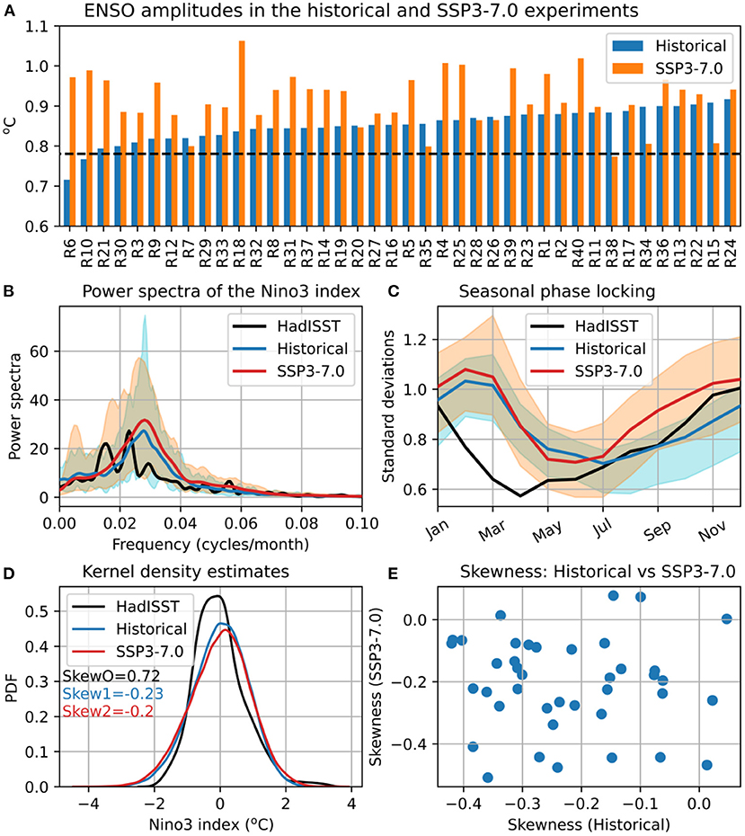
Figure 2. Selected ENSO properties and their changes under global warming as estimated from ACCESS-ESM1.5 large ensembles. (A) ENSO amplitudes (standard deviations of the Niño-3 index) for individual ensemble members of the historical and SSP3-7.0 experiments; the horizontal dashed line indicates the observed amplitude; (B) power spectra; (C) annual variation of ENSO amplitudes; (D) probability density functions; and (E) skewness. The ENSO properties were calculated using the Niño-3 indices from observations (black curve) and the ACCESS-ESM1.5 large ensembles (colored curves). The plotting conventions are as in Figure 1.

The annual variation of ENSO amplitude also shows considerable ensemble spreads (Figure 2C). However, the seasonal phase locking of ENSO, the occurrence of maximum ENSO variability at a particular calendar month, is consistent across the ensemble members. ACCESS-ESM1.5 suffers from a systematic error in its simulated seasonal ENSO phase locking, with the maximum variability occurring in February or March in the historical ensemble, instead of December as for observations. This error was also found in ACCESS-1.3, as mentioned above.

As for the period of ENSO's dominant spectral peak, it is difficult to get the seasonal phase locking right in climate model simulations. Indeed, the majority of the 42 CMIP5 models studied by Rashid and Hirst (2016) showed the maximum ENSO variability occurring in months other than December. Due to this phase locking bias, the simulated ENSO variability is larger than the observed variability during the first half of the calendar year. The ensemble-mean ENSO variability in SSP3-7.0 is similar to that in the historical experiment during the first half of the year but increases significantly during the second half of the year, with the largest increase (~0.16°C) occurring in October. The ensemble spread in the annual cycle of projected ENSO amplitudes tends to be smaller in the middle of the year, and the annual-mean (i.e., averaged over all calendar months) spread is about 33% larger in projections than in the historical simulations. The projected peak ENSO variability occurs mostly in February and March (as for the historical simulations), but eight of the ensemble members now show correct phase locking with the peak variability occurring in December.

It is of interest to see if or how the probability distributions of ENSO-related SST anomalies are affected by the global warming. Figure 2D shows the kernel density estimates (KDEs) of the Niño-3 indices from observations and the historical and SSP3-7.0 simulations. We have chosen KDEs over histograms for clarity of presentations. The observed Niño-3 index has a well-known positively skewed distribution (black curve), with the extreme El Niño events being stronger than the extreme La Niña events. On the other hand, the simulated Niño-3 indices show negative ensemble-mean skewness for both the historical and SSP3-7.0 experiments. The individual ensemble members, however, show a wide range of skewness: −0.42 to 0.05 for the historical experiment and −0.51 to 0.08 for the SSP3-7.0 experiment (Supplementary Figure S3). This negative skewness bias implies that the simulated La Niña events are stronger than the El Niño events in both experiments, in contrast to the observational result. There is no significant difference in ensemble-mean skewness between the historical and SSP3-7.0 ensembles, and there is also no significant correlation between the skewness values of individual members in these ensembles (Figure 2E). The negative skewness bias is seen in many CMIP models, for which several mechanisms have been proposed in the literature. These mechanisms include the cold bias in simulated Pacific mean-state SSTs (leading to weak positive non-linear air-sea interaction), a weak subsurface non-linear dynamic heating in the ocean, and non-linear atmospheric feedbacks (Frauen and Dommenget, 2010; Sun et al., 2016; Hayashi et al., 2020). However, we haven't found any correlation between the central equatorial Pacific cold bias and skewness in the ACCESS-ESM1.5 ensemble members (not shown).

Causes of the uncertainty in ENSO amplitude change under global warming

It is well-known that the ENSO-driven SST variability is governed by the atmosphere-ocean coupling processes in the tropical Pacific (see Timmermann et al., 2018 for a recent review). The processes that most significantly contribute to ENSO's growth and phase transition are surface wind responses to the equatorial eastern Pacific SST variations (the Bjerknes or zonal wind feedback), the zonal advection of mean SSTs by the anomalous current (the zonal advective feedback) and the vertical advection of anomalous subsurface temperatures by the mean upwelling (the thermocline feedback). The two latter feedbacks are related to the ocean dynamic responses to zonal wind forcing that cause in-phase variations of eastern Pacific SST anomalies (Jin and An, 1999; Kim et al., 2014). A diagnostic quantity that encapsulates both these feedback processes is the zonal wind forcing of SST anomalies, which was found to be useful for studying ENSO-amplitude changes under GW (Rashid et al., 2016).

Figure 3 shows quantities related to the Bjerknes feedback, zonal wind forcing and thermocline feedback, computed as lag-regression coefficients between the SST and thermocline depth anomalies averaged over the Niño-3 region and ZWS anomalies averaged over the Niño-4 region. In each panel, regression coefficients between two variables at different lags are plotted for observations and the historical and SSP3-7.0 experiments. For the two experiments, the ensemble medians and spreads (the 5th−95th percentile range) are plotted. The top panel shows the Niño-4 ZWS responses to the Niño-3 SST indices (i.e., the Bjerknes feedback). As in many other CMIP models (e.g., Bellenger et al., 2014), the simulated ZWS responses in ACCESS-ESM1.5 are a lot weaker than the observed response (Figure 3A). The strength of the feedback increases for lags between −5 and 5 months in the SSP3-7.0 experiment relative to the historical experiment but still remains significantly weaker than the observed strength. Note that the Bjerknes feedback is conventionally defined as the zero-lag regression of ZWS on to the SSTs; we do the same in the subsequent analysis. The middle panel (Figure 3B) shows the Niño-3 SST responses to the Niño-4 ZWS anomalies (i.e., the zonal wind forcing). In this case, the simulated SST responses are somewhat stronger than the observed response, and the maximum responses are found at small positive lags (e.g., when ZWS leads SST by 2–3 months). The ZWS forcing is defined as the maximum regression coefficients (at 2–3 month leads) (Rashid et al., 2016), which also strengthens under GW, as for the Bjerknes feedback. The thermocline-SST coupling coefficients, obtained by regressing the Niño-3 SST anomalies onto the thermocline anomalies in the same region, is shown in the bottom panel. As for the Bjerknes feedback and ZWS forcing discussed above, only the coupling strengths at zero or positive lags (i.e., when the thermocline anomalies lead) are related to the thermocline feedback. The thermocline feedback, thus defined, peaks at the 2-months lead for observations and at 6- and 5-months leads for the historical and SSP3-7.0 simulations, respectively. The peak (0.036°C/m) of the historical ensemble median feedbacks is close to the observed value (0.038°C/m), and the peak (0.043°C/m) of the SSP3-7.0 ensemble median feedbacks is stronger than the corresponding historical value (Figure 3C). However, this strengthening of the thermocline feedback under GW is less clear-cut, as the ensemble spreads for the two experiments overlap at all lags.

FIGURE 3

Figure 3. Lag-regression coefficients of ENSO variables related to the key ENSO processes, and their changes under global warming. (A) Regression of the Niño-4 zonal wind stress index onto the Niño-3 SST index (related to the atmospheric Bjerknes feedback), (B) regression of the Niño-3 SST index onto the Niño-4 zonal wind stress index (related to the zonal wind forcing of SST), and (C) regression of the Niño-3 SST index onto the Niño-3 thermocline depth index (related to the thermocline feedback). The colored thick curves represent the ensemble medians and the shadings indicate the respective 5–95% confidence intervals, both estimated from the 40 ensemble members. In each plot, the first variable leads the second variable at positive lags.

The relationship between the changes in these ENSO processes and those in ENSO amplitude is illustrated in Figure 4 using scatter diagrams. The zonal gradient of time-mean SSTs in the Pacific also is an important controlling factor for ENSO variability, so we examine its relationship with ENSO amplitude, as well. There is a significant correlation between the simulated ENSO amplitudes and mean zonal SST gradients for different ensemble members, indicating an increasing ENSO amplitude with decreasing magnitude of the SST gradient, and vice-versa (Figure 4A). The correlation is moderate in the historical ensemble (r = 0.54), which becomes significantly stronger in the SSP3-7.0 ensemble (r = 0.81). The observed SST difference (Niño-3 minus Niño-4) is −2.69°C, which is substantially larger than the ensemble-mean value (−1.82°C) of the historical ensemble. The SSP3-7.0 ensemble-mean value (−1.81°C) remains largely unchanged from the historical ensemble-mean value, but the ensemble spread increases under GW.

FIGURE 4

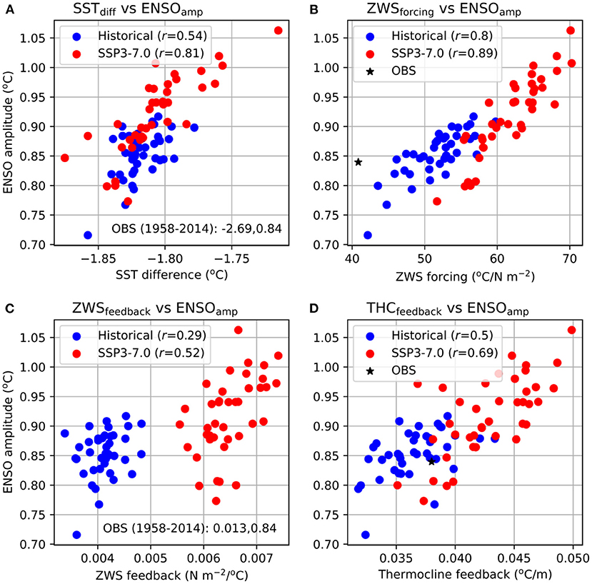
Figure 4. Relationship between the key ENSO processes and ENSO amplitudes, as calculated from observations and individual simulations of the ACCESS-ESM1.5 historical and SSP3-7.0 large ensembles. ENSO amplitudes vs. (A) differences of mean SSTs between the Niño-3 and Niño-4 regions (as a proxy for the zonal SST gradient), (B) the zonal wind forcings of ENSO-related SST anomalies, (C) the Bjerknes feedbacks, and (D) the thermocline feedbacks. The correlation coefficients for each experiment are shown in the legends. In (A,C), the observed values are shown as texts (as the values are very large compared to the simulated values, so these cannot be conveniently plotted); in (B,D), the observed values are plotted as an asterisk.

Figure 4B shows the relationship between ENSO amplitudes and the ZWS forcings for individual members of the historical and SSP3-7.0 ensembles. The ZWS forcing is defined as the maximum of R(Tauu,SST) values at positive lags; see Figure 3B. There is a high correlation between the ZWS forcings and ENSO amplitudes across the members of each ensemble. The already high correlation (r = 0.8) for the historical ensemble becomes even higher in the SSP3-7.0 ensemble (r = 0.89), indicating an intimate relationship between the ZWS forcing and ENSO amplitude that strengthens further under GW. This is consistent with the result of a previous analysis of the pre-industrial control and abrupt-4xCO2 simulations from CMIP5 (Rashid et al., 2016). Unlike for the SST gradient (and the Bjerknes feedback to be discussed next), the ZWS forcings in the historical ensemble (mean = 51.7°C/N m⁻²) are stronger than the observed value (40.8°C/N m⁻²), and the SSP3-7.0 ensemble-mean (61.8°C/N m⁻²) is even stronger. Among the four ENSO-related processes considered here, the ZWS forcing has the largest influence on simulated ENSO amplitudes. The Bjerknes feedbacks show a weak correlation (r = 0.29) with ENSO amplitudes in the historical ensemble, which strengthens to a moderate correlation (r = 0.52) in the SSP3-7.0 ensemble (Figure 4C). The simulated Bjerknes feedbacks (ensemble-mean = 0.004 N m⁻²/°C) are less than half of the observed value (0.013 N m⁻²/°C), a bias also experienced by other climate models (e.g., Bellenger et al., 2014). The ensemble means of the thermocline feedback (defined as the maximum of R(THD,SST) values at positive lags) for the historical and SSP3-7.0 experiments are 0.036 and 0.043°C/m, respectively; these are comparable to the observed value (0.038°C/m). The simulated feedbacks are moderately to highly correlated with ENSO amplitudes in the historical and SSP3-7.0 ensembles, with r = 0.5 and 0.69, respectively (Figure 4D).

Therefore, all four processes show correlations with ENSO amplitudes across the members of two large ensembles of ACCESS-ESM1.5, with the lowest correlations found for the Bjerknes feedbacks and the highest for the ZWS forcing. In all four cases, the correlation coefficient increases from the historical to the SSP3-7.0 ensemble, with the highest increase occurring for the Bjerknes feedback–ENSO amplitude correlation (~79%) and lowest increase for the ZWS forcing-ENSO amplitude correlation (~11%). Note, however, that these two increases occur from the lowest and highest historical correlations, respectively.

The differences in SSP3-7.0 and historical ensemble means, discussed above, indicate GHG forced changes in the ENSO amplitude and processes. However, there are significant ensemble variations (due to internal variability) in these GHG forced changes. The relative contributions of the ENSO processes to the ensemble variation of ENSO amplitude change can be estimated using a multiple linear regression (MLR) analysis:

$\begin{array}{l}dENS{O}_{amp}=a+b\ast dSS{T}_{grad}+c\ast dZW{S}_{forcing}\\ +d\ast dZW{S}_{feedback}+e\ast dTH{D}_{feedback}+R\end{array}$

where, the prefix “d” indicates changes in the dependent and independent variables from the historical to the SSP3-7.0 experiment, expressed as percentages of the respective historical values. The variables are vectors consisting of the changes in relevant statistics in 40 ensemble members (shown as dots in Figure 4), R is the residual vector, a is the intercept term, and b, c, d, and e are the regression coefficients. In the ideal case of the independent variables (or predictors) being uncorrelated to each other, the sum of the partial variances explained by the four processes plus the residual variance would be equal to the ensemble-variance of the ENSO amplitude changes. However, the independent variables do have low to moderate mutual correlations (|r| = 0.3–0.54), resulting in a “covariance” contribution. In our analysis, this covariance contribution is ~25% of the total ENSO amplitude variance (see below), which is less than half of the sum of individual variances explained by the four processes (~58%). The effect of these mutual correlations (or, multicollinearity) can also be quantified by the variance inflation factors (VIFs). The VIFs for our MLR model range from 1.37–1.86, which are far less than the threshold VIF value of 5, above which the multicollinearity becomes problematic (e.g., James et al., 2013). Therefore, this MLR model can be useful in providing information about relative contributions of the processes; a similar model has been effectively used in some other recent analyses (Rashid, 2021; Rashid et al., 2022).

The result of the MLR analysis is presented in Figure 5. The four ENSO processes and their covariations together explain about 83% of the ensemble variance of ENSO amplitude changes (dENSO_amp), leaving ~17% as the residual variance. There is a wide range of values for dENSO_amp across the ensemble members (−13–36%), with eight of the 40 members showing a reduction in ENSO amplitude from the historical to the SSP3-7.0 experiment (Figure 5A, black curve). That is, the ensemble variation of 49% in dENSO_amp is more than six times larger than its ensemble mean (7.8%), indicating the internal variability dominates the forced ENSO amplitude change in ACCESS-ESM1.5. The MLR predicted dENSO_amp for different ensemble members and the associated residuals are also shown in Figure 5A. As expected from the high explained variance (83%) mentioned above, the predicted components are fairly similar to the full dENSO_amp, with small residual values. The computed regression coefficients for the four processes and their 5–95% confidence intervals (estimated from a two-sided t-test) are shown in Figure 5B. The coefficients for dSST_grad and dZWS_forcing are found to be statistically significant at the 95% level, whereas the other two coefficients, for dZWS_feedback and dTHD_feedback, are not significantly different from zero. The negative regression coefficient for dSST_grad results from the fact that reduced SST gradients in the SSP3-7.0 experiment (relative to the historical experiment) are associated with enhanced ENSO amplitudes, and vice-versa (cf. Figure 4A). The percentage variances of dENSO_amp explained by the four processes are shown in Figure 5C. The largest contribution comes from dZWS_forcing (~43%), with the second largest contribution coming from the covariation of all four processes (~25%). The mean-state change, dSST_grad, contributes around 14% to dENSO_amp, with the other two processes contributing negligible amounts (consistent with Figure 5B).

FIGURE 5

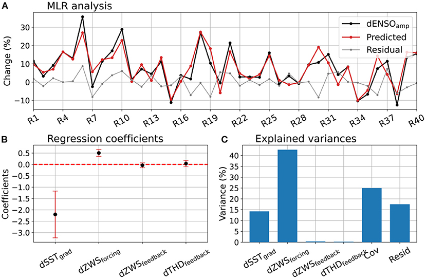
Figure 5. Contributions of different ENSO processes to the ensemble variation of ENSO amplitude changes under global warming, as assessed by a multiple linear regression (MLR) model. (A) ENSO amplitude changes in different ensemble members (black curve), ENSO amplitude changes predicted by the MLR (red curve), and the residuals (gray curve); (B) the regression coefficients and their 5–95% confidence intervals (estimated by a two-sided t-test); and (C) percentage (ensemble) variances of ENSO amplitude changes explained by different ENSO processes, as well as the covariance and residual contributions. The GW-induced changes (SSP3-7.0 minus historical) for different ensemble members are expressed as percentages of the respective historical experiment member.

The fact that the covariance contribution is the second largest component suggests this result should be interpreted with caution. We suspect that the near-zero variance contributions from dZWS_feedback and dTHD_feedback are an artifact of this substantial covariation between the predictors. In other words, these two processes do actually have non-zero (albeit small) contributions to the GW-induced changes in ENSO amplitude (Supplementary Figure S4), but these are absorbed into the covariance contribution. This can happen if their ensemble variations are correlated with the variations of the other more dominant processes, which is the case here. Nevertheless, the result discussed above is consistent with the result presented in Figure 4, where SST_grad and ZWS_forcing were found to have the largest correlations with ENSO amplitudes across ensemble members. Also, their changes under GW have the two largest correlations with ENSO amplitude changes (Supplementary Figure S4).

Summary and discussions

In this work, we have analyzed and documented the responses of ENSO to the combined GHG and aerosol forcings using ACCESS-ESM1.5 LEs for CMIP6 historical and SSP3-7.0 experiments. Previous studies with multi-model and single-model LEs showed significant internal variability generated uncertainties in the forced response of ENSO. Here, for the first time, we quantify the response uncertainty using ACCESS-ESM1.5 LEs and investigate the processes responsible for this uncertainty. We find substantial ensemble spreads in ENSO's amplitude, power spectrum, and skewness (Figure 2). The ensemble mean amplitude increases by about 8% in the SSP3-7.0 experiment relative to the historical experiment and this increase is statistically significant according to a two-sided t-test (p = 1.5 × 10⁻⁶) and a separate bootstrap resampling test. There is also a wide range of changes (−13–36%) across the ensemble members (Figures 2A, 5A). Consistently, the ensemble-mean power spectrum shows enhanced power in the SSP3-7.0 experiment compared to the historical experiment, mostly around the 3-year period where the mean ENSO spectral peak is located (Figure 2B); this enhancement is smaller than the ensemble spreads of both experiments. There appears to be no significant difference in ensemble-mean skewness between the two experiments (Figure 2D).

The mechanism of GW-induced changes in ENSO amplitude is investigated in terms of the changes in prominent ENSO feedbacks and forcing. The largest percentage changes happen in the Bjerknes feedback, but these changes are not highly correlated (across ensemble members) with ENSO amplitude changes (Figure 4C and Supplementary Figure S4). Rather, the latter are best correlated with changes in the ZWS forcing (r = 0.85) and mean SST gradient (r = −0.72) (Supplementary Figure S4). The relative contributions to the ensemble variation (i.e., uncertainty due to internal variability) of ENSO amplitude changes from the changes in four processes are quantified using an MLR model. The results from this MLR model confirm the dominant role of the ZWS forcing (and mean SST gradient), with the caveat that about 25% of the ensemble variance of ENSO amplitude changes arise from covariations of the four processes (Figure 5). The ZWS forcing is, in turn, linked with the zonal wind–convection coupling strength in the central-western equatorial Pacific region (Supplementary Figure S5). The surface westerlies in this region are coupled, through convergence, with the local convection. This coupling is strong in observations, with a high correlation between the Niño-4 ZWS and rainfall anomalies (r = 0.74). The strength of this coupling is much weaker in ACCESS-ESM1.5 historical simulations, with an ensemble correlation coefficient of 0.35. However, the correlation increases significantly in the SSP3-7.0 simulations (r = 0.58), presumably because of the associated background state warming in the equatorial Pacific. This explains the dominance of GW-induced changes in the ZWS forcing on ENSO amplitude changes discussed above. This result is not unique to ACCESS-ESM1.5 simulations; similar results were found in a subset of CMIP5 models that showed ENSO amplitude increases in the abrupt-4xCO2 experiment (Rashid et al., 2016). However, whether a similar mechanism works in nature is not clear.

As shown above, the GW signal (as defined by the ensemble mean) in ENSO amplitude is small (but statistically significant) compared to its variation due to internal variability. However, a stronger signal may be found if the ENSO amplitude change is examined in a scenario experiment with much stronger radiative forcing, e.g., the CMIP6 SST5-8.5 experiment. Another issue is that the GHG forcings gradually increase over a period (2015–2100) in these experiments, so the simulated ENSO variability does not experience the same level of external forcings over the whole period. This could be addressed using scenario runs extended to year 2300 with forcings stabilized at the year 2100 level.

Nevertheless, as mentioned above, the single-model ensemble results reported here are consistent with those found from a multi-model ensemble of CMIP5 models using a different set of experiments, the pre-industrial control and abrupt-4xCO2 experiments (Rashid et al., 2016). These CMIP5 models also showed a small ensemble-mean increase in ENSO amplitude under GW, a large ensemble variation, the dominant role of ZWS forcing in this variation and a strong connection to the zonal wind–deep convection coupling. This consistency of results between different generations of models and between different sets of experiments indicates the robustness of the results. Note that some studies reporting robust increases of ENSO amplitude under GW choose a subset of CMIP5 models using one or more criteria that may be debatable, although most of the CMIP6 models show an increase (Fredriksen et al., 2020; Grose et al., 2020; Cai et al., 2022). However, even the ensemble-mean increase shown by the CMIP6 models is still modest compared to the inter-model variation of ENSO amplitude change. This highlights the importance of understanding this variation, which is a focus of this study.

Data availability statement

Publicly available datasets were analyzed in this study. This data can be found at: The ACCESSESM1.5 model outputs for CMIP6 used in this study may be downloaded freely from https://esgf-node.llnl.gov/projects/cmip6/ upon registration. The HadISST data was obtained from: https://www.metoffice.gov.uk/hadobs/hadisst/data/download.html. The ERA5 reanalysis products are from: https://cds.climate.copernicus.eu/#!/search?text=ERA5&type=dataset. The ORAS4 reanalysis is available at: http://apdrc.soest.hawaii.edu:80/dods/public_data/Reanalysis_Data/ORAS5/1x1_grid/votemper/opa4.

Author contributions

HR conceives the research idea, performed data analysis, interpreted the results, and wrote the manuscript.

Funding

This work has been partially funded by Australia's National Environmental Science Programme. The ACCESS model simulations for CMIP6 were performed using the resources and services from the National Computational Infrastructure (NCI), which was supported by the Australian Government.

Acknowledgments

I thank the official reviewers for providing insightful comments on the submitted manuscript. I thank the ACCESS model development team for performing the climate and earth system simulations for CMIP6, some of which are used in this study. I especially thank Dr. Tilo Ziehn for planning and performing the large ensemble simulations with ACCESS-ESM1.5.

Conflict of interest

The author declares that the research was conducted in the absence of any commercial or financial relationships that could be construed as a potential conflict of interest.

Publisher's note

All claims expressed in this article are solely those of the authors and do not necessarily represent those of their affiliated organizations, or those of the publisher, the editors and the reviewers. Any product that may be evaluated in this article, or claim that may be made by its manufacturer, is not guaranteed or endorsed by the publisher.

Supplementary material

The Supplementary Material for this article can be found online at: https://www.frontiersin.org/articles/10.3389/fclim.2022.954449/full#supplementary-material

References

Balmaseda, M. A., Mogensen, K., and Weaver, A. T. (2013). Evaluation of the ECMWF ocean reanalysis system ORAS4. Quart. J. R. Meteorol. Soc. 139, 1132–1161. doi: 10.1002/qj.2063

PubMed Abstract | CrossRef Full Text | Google Scholar

Battisti, D., and Hirst, A. (1989). Interannual variability in a tropical atmosphere–ocean model: influence of the basic state, ocean geometry, and nonlinearity. J.Atmos. Sci. 46, 1687–1712.

Google Scholar

Bayr, T., Latif, M., Dommenget, D., Wengel, C., Harlaß, J., and Park, W. (2018). Mean-state dependence of ENSO atmospheric feedbacks in climate models. Clim. Dyn. 50, 3171–3194. doi: 10.1007/s00382-017-3799-2

CrossRef Full Text | Google Scholar

Bellenger, H., Guilyardi, E., Leloup, J., Lengaigne, M., and Vialard, J. (2014). ENSO representation in climate models: from CMIP3 to CMIP5. Clim. Dyn. 42, 1999–2018. doi: 10.1007/s00382-013-1783-z

CrossRef Full Text | Google Scholar

Bjerknes, J. (1969). Atmospheric teleconnections from the equatorial pacific. Month. Weather Rev. 97, 163–172. doi: 10.1175/1520-0493(1969)097<0163:ATFTEP>2.3.CO

CrossRef Full Text | Google Scholar

Cai, W., Ng, B., Wang, G., Santoso, A., Wu, L., and Yang, K. (2022). Increased ENSO sea surface temperature variability under four IPCC emission scenarios. Nat. Clim. Change 12, 228–231. doi: 10.1038/s41558-022-01282-z

CrossRef Full Text | Google Scholar

Cai, W., Santoso, A., Collins, M., Dewitte, B., Karamperidou, C., Kug, J. S., et al. (2021). Changing El Niño–Southern oscillation in a warming climate. Nat. Rev. Earth Environ. 2, 0123456789. doi: 10.1038/s43017-021-00199-z

CrossRef Full Text | Google Scholar

Callahan, C. W., Chen, C., Rugenstein, M., Bloch-Johnson, J., Yang, S., and Moyer, E. J. (2021). Robust decrease in El Niño/Southern oscillation amplitude under long-term warming. Nat. Clim. Change 11, 752–757. doi: 10.1038/s41558-021-01099-2

CrossRef Full Text | Google Scholar

Chen, L., Li, T., and Yu, Y. (2015). Causes of strengthening and weakening of ENSO amplitude under global warming in four CMIP5 models. J. Clim. 28, 3250–3274. doi: 10.1175/JCLI-D-14-00439.1

CrossRef Full Text | Google Scholar

Chen, L., Li, T., Yu, Y., and Behera, S. K. (2017). A possible explanation for the divergent projection of ENSO amplitude change under global warming. Clim. Dyn. 49, 3799–3811. doi: 10.1007/s00382-017-3544-x

CrossRef Full Text | Google Scholar

Collins, M., An, S.-I., Cai, W., Ganachaud, A., Guilyardi, E., Jin, F.-F., et al. (2010). The impact of global warming on the tropical Pacific Ocean and El Nino. Nat. Geosci. 3, 391–397. doi: 10.1038/ngeo868

CrossRef Full Text | Google Scholar

Dee, D. P., Uppala, S. M., Simmons, A. J., Berrisford, P., Poli, P., Kobayashi, S., et al. (2011). The ERA-interim reanalysis: configuration and performance of the data assimilation system. Quart. J. R. Meteorol. Soc. 137, 553–597. doi: 10.1002/qj.828

CrossRef Full Text | Google Scholar

Deser, C., Lehner, F., Rodgers, K. B., Ault, T., Delworth, T. L., DiNezio, P. N., et al. (2020). Insights from Earth system model initial-condition large ensembles and future prospects. Nat. Clim. Change 10, 277–286. doi: 10.1038/s41558-020-0731-2

CrossRef Full Text | Google Scholar

Eyring, V., Bony, S., Meehl, G. A., Senior, C. A., Stevens, B., Stouffer, R. J., et al. (2016). Overview of the coupled model intercomparison project phase 6 (CMIP6) experimental design and organization. Geosci. Model Develop. 9, 1937–1958. doi: 10.5194/gmd-9-1937-2016

CrossRef Full Text | Google Scholar

Frauen, C., and Dommenget, D. (2010). El Niño and la Niña amplitude asymmetry caused by atmospheric feedbacks. Geophys. Res. Lett. 37, 1–6. doi: 10.1029/2010GL044444

CrossRef Full Text | Google Scholar

Fredriksen, H. B., Berner, J., Subramanian, A. C., and Capotondi, A. (2020). How does El Niño–Southern oscillation change under global warming—a first look at CMIP6. Geophys. Res. Lett. 47, e2020GL090640. doi: 10.1029/2020GL090640

CrossRef Full Text | Google Scholar

Gill, A. E., and Rasmusson, E. M. (1983). The 1982-83 climate anomaly in the equatorial Pacific. Nature 306, 229–234.

Google Scholar

Grose, M. R., Narsey, S., Delage, F. P., Dowdy, A. J., Bador, M., Boschat, G., et al. (2020). Insights from CMIP6 for Australia's future climate. Earths Fut. 8, e2019EF001469. doi: 10.1029/2019EF001469

CrossRef Full Text | Google Scholar

Ham, Y. G., and Kug, J. S. (2016). ENSO amplitude changes due to greenhouse warming in CMIP5: role of mean tropical precipitation in the twentieth century. Geophys. Res. Lett. 43, 422–430. doi: 10.1002/2015GL066864

CrossRef Full Text | Google Scholar

Hayashi, M., Jin, F. F., and Stuecker, M. F. (2020). Dynamics for El Niño-La Niña asymmetry constrain equatorial-Pacific warming pattern. Nat. Commun. 11, 1–10. doi: 10.1038/s41467-020-17983-y

PubMed Abstract | CrossRef Full Text | Google Scholar

Hersbach, H., Bell, B., Berrisford, P., Hirahara, S., Horányi, A., Muñoz-Sabater, J., et al. (2020). The ERA5 global reanalysis. Quart. J. R. Meteorol. Soc. 146, 1999–2049. doi: 10.1002/qj.3803

CrossRef Full Text | Google Scholar

Hyun, S., Yeh, S.-W., Kirtman, B. P., and An, S.-I. (2022). Internal climate variability in the present climate and the change in ENSO amplitude in future climate simulations. Front. Clim. 4, 932978. doi: 10.3389/fclim.2022.932978

CrossRef Full Text | Google Scholar

James, G., Witten, D., Hastie, T., and Tibshirani, R. (2013). An Introduction to Statistical Learning, Vol. 112. New York, NY: Springer. doi: 10.1007/978-1-4614-7138-7

CrossRef Full Text | Google Scholar

Jin, F., and An, S. (1999). Thermocline and zonal advective feedbacks within the equatorial ocean recharge oscillator model for ENSO. Geophys. Res. Lett. 26, 2989–2992.

Google Scholar

Jin, F.-F. (1997). An equatorial ocean recharge paradigm for ENSO. Part I: conceptual model pacific from his analysis of the empirical relations of. J. Atmos. Sci. 54, 811–829.

Google Scholar

Kim, S. T., Cai, W., Jin, F. F., and Yu, J. Y. (2014). ENSO stability in coupled climate models and its association with mean state. Clim. Dyn. 42, 3313–3321. doi: 10.1007/s00382-013-1833-6

CrossRef Full Text | Google Scholar

Mackallah, C., Chamberlain, M. A., Law, R. M., Dix, M., Ziehn, T., Bi, D., et al. (2022). ACCESS datasets for CMIP6: methodology and idealised experiments. J. South. Hemisphere Earth Syst. Sci. 299, 1–24. doi: 10.1071/ES21031

CrossRef Full Text | Google Scholar

Maher, N., Matei, D., Milinski, S., and Marotzke, J. (2018). ENSO change in climate projections: forced response or internal variability? Geophys. Res. Lett. 45, 390–398. doi: 10.1029/2018GL079764

CrossRef Full Text | Google Scholar

Ng, B., Cai, W., Cowan, T., and Bi, D. (2021). Impacts of low-frequency internal climate variability and greenhouse warming on El Niño–Southern oscillation. J. Clim. 34, 2205–2218. doi: 10.1175/JCLI-D-20-0232.1

CrossRef Full Text | Google Scholar

O'Neill, B. C., Tebaldi, C., Van Vuuren, D. P., Eyring, V., Friedlingstein, P., Hurtt, G., et al. (2016). The scenario model intercomparison project (ScenarioMIP) for CMIP6. Geosci. Model Develop. 9, 3461–3482. doi: 10.5194/gmd-9-3461-2016

CrossRef Full Text | Google Scholar

Philip, S., and van Oldenborgh, G. J. (2006). Shifts in ENSO coupling processes under global warming. Geophys. Res. Lett. 33, L11704. doi: 10.1029/2006GL026196

CrossRef Full Text | Google Scholar

Planton, Y. Y., Guilyardi, E., Wittenberg, A. T., Lee, J., Gleckler, P. J., Bayr, T., et al. (2020). Evaluating climate models with the CLIVAR 2020 ENSO metrics package. Bull. Am. Meteorol. Soc. 102, E193–E217. doi: 10.1175/BAMS-D-19-0337.1

CrossRef Full Text | Google Scholar

Rashid, H. A. (2021). Diverse responses of global-mean surface temperature to external forcings and internal climate variability in observations and CMIP6 models. Geophys. Res. Lett. 48, 1–11. doi: 10.1029/2021GL093194

CrossRef Full Text | Google Scholar

Rashid, H. A., and Hirst, A. C. (2016). Investigating the mechanisms of seasonal ENSO phase locking bias in the ACCESS coupled model. Clim. Dyn. 46, 1075–1090. doi: 10.1007/s00382-015-2633-y

CrossRef Full Text | Google Scholar

Rashid, H. A., Hirst, A. C., and Marsland, S. J. (2016). An atmospheric mechanism for ENSO amplitude changes under an abrupt quadrupling of CO2 concentration in CMIP5 models. Geophys. Res. Lett. 43, 1687–1694. doi: 10.1002/2015GL066768

CrossRef Full Text | Google Scholar

Rashid, H. A., Sullivan, A., Dix, M., Bi, D., Mackallah, C., Ziehn, T., et al. (2022). Evaluation of climate variability and change in ACCESS historical simulations for CMIP6. J. Southern Hemisphere Earth Syst. Sci. 1–20. doi: 10.1071/ES21028. [Epub ahead of print].

CrossRef Full Text | Google Scholar

Rashid, H. A., Sullivan, A., Hirst, A. C., Bi, D., Zhou, X., and Marsland, S. J. (2013). Evaluation of El Niño – southern oscillation in the ACCESS coupled model simulations for CMIP5. Aust. Meteorol. Oceanogr. J. 63, 161–180. doi: 10.22499/2.6301.010

CrossRef Full Text | Google Scholar

Rasmusson, E. M., and Carpenter, T. H. (1982). Variations in tropical sea surface temperature and surface wind fields associated with the Southern Oscillation/El Niño. Monthly Weather Rev. 110, 354–384.

Google Scholar

Rayner, N. A., Parker, D. E., Horton, E. B., Folland, C. K., Alexander, L. V., Rowell, D. P., et al. (2003). Global analyses of sea surface temperature, sea ice, and night marine air temperature since the late nineteenth century. J. Geophys. Res. Atmos. 108, 1–29. doi: 10.1029/2002JD002670

CrossRef Full Text | Google Scholar

Sun, Y., Wang, F., and Sun, D. Z. (2016). Weak ENSO asymmetry due to weak nonlinear air–sea interaction in CMIP5 climate models. Adv. Atmos. Sci. 33, 352–364. doi: 10.1007/s00376-015-5018-6

CrossRef Full Text | Google Scholar

Taylor, K. E., Stouffer, R. J., and Meehl, G. A. (2012). An overview of CMIP5 and the experiment design. Bull. Am. Meteorol. Soc. 93, 485–498. doi: 10.1175/BAMS-D-11-00094.1

PubMed Abstract | CrossRef Full Text | Google Scholar

Timmermann, A., An, S. II., Kug, J. S., Jin, F. F., Cai, W., Capotondi, A., et al. (2018). El Niño–southern oscillation complexity. Nature 559, 535–545. doi: 10.1038/s41586-018-0252-6

PubMed Abstract | CrossRef Full Text | Google Scholar

Wallace, J. M., Rasmusson, E. M., Mitchell, T. P., Kousky, V. E., Sarachik, E. S., and von Storch, V. (1998). On the structure and evolution of climate variability in the tropical Pacific: lessons from TOGA. J. Geophys. Res. 103, 14241–14259.

Google Scholar

Ying, J., Huang, P., Lian, T., and Chen, D. (2019). Intermodel uncertainty in the change of ENSO's amplitude under global warming: role of the response of atmospheric circulation to SST anomalies. J. Clim. 32, 369–383. doi: 10.1175/JCLI-D-18-0456.1

CrossRef Full Text | Google Scholar

Zebiak, S. E., and Cane, M. A. (1987). A model El Nino-southern oscillation. Monthly Weather Rev. 115, 2262–2278.

Google Scholar

Zheng, X. T., Hui, C., and Yeh, S. W. (2018). Response of ENSO amplitude to global warming in CESM large ensemble: uncertainty due to internal variability. Clim. Dyn. 50, 4019–4035. doi: 10.1007/s00382-017-3859-7

CrossRef Full Text | Google Scholar

Ziehn, T., Chamberlain, M. A., Law, R. M., Lenton, A., Bodman, R. W., Dix, M., et al. (2020). The Australian earth system model: ACCESS-ESM1.5. J. Southern Hemisphere Earth Syst. Sci. 70, 193–214. doi: 10.1071/ES19035

CrossRef Full Text | Google Scholar