 Dudsadee Leenawarat
 Jutarak Luang-on
 Anukul Buranapratheprat2
 Joji Ishizaka
- 1Department of Earth and Environmental Sciences, Graduate School of Environmental Studies, Nagoya University, Nagoya, Japan
- 2Department of Aquatic Science, Faculty of Science, Burapha University, Chonburi, Thailand
- 3Institute for Space-Earth Environmental Research (ISEE), Nagoya University, Nagoya, Japan
This study investigated the seasonal variability of surface chlorophyll-a (chl-a) and the influence of the El Niño Southern Oscillation (ENSO) related to environmental parameters in the Gulf of Thailand (GoT). Monthly chl-a data from MODIS from 2002 to 2020 as well as sea surface temperature (SST), wind, precipitation, and river discharge were used in this analysis. Results from seasonal climatology and Empirical Orthogonal Function (EOF) described high chl-a concentration areas along the western to the southern coasts and near Ca Mau Cape during the northeast monsoon (NEM), and the upper GoT (UGoT), eastern coast, and the GoT mouth during the southwest monsoon (SWM), while low chl-a took place during the non-monsoon (NON). The GoT was divided into six areas based on the EOFs of chl-a, and then the correlation between chl-a variability and environmental parameters was also examined. The results suggested that chl-a in coastal and offshore areas were controlled by different mechanisms. Chl-a in coastal areas responded to precipitation and river discharge as well as the shoreward wind; meanwhile, chl-a in offshore areas correlated with SST and wind magnitude indicating the importance of water mixing and upwelling. The fluctuation of chl-a in each season related to ENSO was captured by EOF based on the seasonal anomaly. The influence of ENSO was strong during NEM and NON but minimal during SWM. El Niño/La Niña generally caused low/high precipitation and high/low SST. Moreover, El Niño/La Niña caused anomalously weak/strong wind during NEM contrary to during NON. Anomalous high/low chl-a were observed in shallow regions during El Niño/La Niña corresponding to strong/weak wind in NON. Abnormal wind under ENSO also created the shifting in the high chl-a area near Ca Mau Cape. These results have improved our understanding of monsoons and ENSO variabilities as the crucial drivers of changes in the tropical marine ecosystem in both seasonal and interannual time scales.
Introduction
The monsoon system is a major climate driver in the tropical region, causes wet and dry conditions, and plays an important role in oceanographic processes on the annual time scale (Wyrtki, 1961; Robinson, 1974). Meanwhile, large-scale phenomena such as El Niño Southern Oscillation (ENSO) and Indian Ocean Dipole (IOD) also modify the monsoon strength (Wang et al., 2009; Li et al., 2016; Kim et al., 2020) and influence the oceanographic processes in the inter-annual time scale (Vinayachandran et al., 2009; Kuo and Tseng, 2020). In shallow seas, the interaction of wind, precipitation, river discharge, heat, and tidal current creates more dynamics than the deeper oceans (Simpson and Sharples, 2012). The dynamics of physical and biological properties in the tropical shelf sea are strongly varied by monsoons, ENSO, and IOD (Tang et al., 2006; Sari et al., 2018b; Huynh et al., 2020; Siswanto et al., 2020; Luang-on et al., 2021; Sripoonpan and Saramul, 2021).
The Gulf of Thailand (GoT; Figure 1) is one of the largest shallow semi-enclosed seas in a tropical region that is influenced by the northeast monsoon (NEM) and the southwest monsoon (SWM). The average depth is approximately 40 m with the deepest around 80 m near the central area. This area stretches in the northwest-southeast direction over the Sunda Shelf, and its sea boundary is defined by a cross line from Ca Mau Cape, Vietnam to Kota Bharu, Malaysia. The GoT is surrounded by Vietnam, Cambodia, Thailand, and Malaysia, which connects to the South China Sea (SCS) via the southeastern part. This whole area is characterized as an estuary that has two water layers (Robinson, 1974; Simpson and Sharples, 2012): (1) low-salinity water mass in the upper layer caused by river discharge and precipitation; (2) low-temperature with high-salinity water mass which intruded from the SCS.
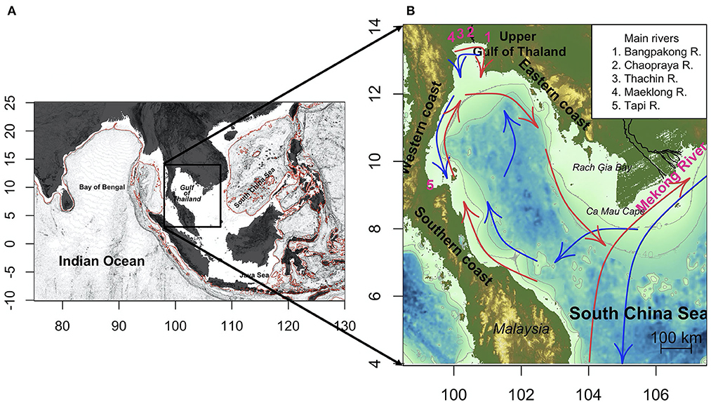
Figure 1. Location (A) and topography (B) of the Gulf of Thailand. The gray contour lines in (B) denote bathymetry at 20 and 40 meters, blue and red vectors indicate the ocean circulation during northeast monsoon and southwest monsoon, respectively (adapted from Buranapratheprat and Bunpapong, 1998).
The oceanographic processes such as ocean circulation, water column conditions, and coastal upwelling under different monsoons have been investigated (Wyrtki, 1961; Robinson, 1974; Yanagi and Takao, 1998; Buranapratheprat et al., 2016; Guo et al., 2021; Sripoonpan and Saramul, 2021). The NEM influences this region from mid-October to mid-February. It induces dry and cold air from Central Asia to this area and causes high precipitation over the southern GoT and the Malay Peninsula (Laonamsai et al., 2020). The well-mixed water column and counterclockwise circulation are developed during this period (Yanagi and Takao, 1998; Chaiongkarn and Sojisuporn, 2013; Buranapratheprat et al., 2016). The east-southeast wind prevails from the SCS to the GoT, then changes direction to the north in the northern area from mid-February to mid-May (non-monsoon; NON) and generates upwelling in some areas (Sripoonpan and Saramul, 2021). The NON coincides with the local summer season resulting in strong stratification during this time (Yanagi and Takao, 1998; Buranapratheprat et al., 2016). Meanwhile, the SWM replaces from mid-May to mid-October and develops clockwise circulation. The SWM brings high precipitation to the mainland resulting in large river runoff in late SWM. The main rivers including Bangpakong, Chaophraya, Thachin, and Maeklong Rivers are located in Upper GoT (UGoT). Just the Tapee River is located in the southern part of the GoT. The influences of freshwater runoff from the Mekong River on the GoT water are also reported (Robinson, 1974; Stansfield and Garrett, 1997). They all are significant as the sources of nutrients and sediments in the GoT (Wattayakorn and Jaiboon, 2014; Shi et al., 2015), supporting phytoplankton growth and primary productivity. However, large freshwater runoff and excess nutrient loads can generate adverse environmental effects including eutrophication, red tide, and hypoxia in this area, specifically in the UGoT (Buranapratheprat et al., 2021; Morimoto et al., 2021; Sukigara et al., 2021).
Although the GoT is known as an important fishing ground (Janetkitkosol et al., 2003; SEAFDEC, 2018; Li et al., 2021), the lower-trophic level ecosystem in this area is not well understood. Most studies are conducted in specific coastal areas, mostly the UGoT. The field observations in the western GoT in 1995–1996 and 2013 heading by the Southeast Asian Fisheries Development Center (SEAFDEC) were conducted to investigate oceanographic condition, marine environment, phytoplankton abundance, species, and distribution (Boonyapiwat, 1998; Saadon et al., 1998; Sompongchaiyakul et al., 2013) but only transition periods of monsoon were observed. Thereafter, Tang et al. (2006) used SeaWiFS data to study the seasonal variation of chlorophyll-a (chl-a) on both sides of the Indochina Peninsula and pointed out the influence of the monsoons and coastal environments on phytoplankton in this area. Chl-a in the GoT has its peak related to well-mixed water, but high chl-a near Ca Mau Cape is related to coastal jet during NEM. Huynh et al. (2020) also reported the influence of NEM on chl-a. They additionally explained the increase of chl-a on the eastern coast during SWM, which was related to the river discharge and the southwest wind. However, it is still unclear that how freshwater is transported to the east coast because the main rivers are located in the UGoT, and the river discharge reaches its peak in late SWM (September to October) (Stansfield and Garrett, 1997). Luang-on et al. (2021) then revealed the relationship between chl-a and environmental parameters, including precipitation, river discharge, and wind under influence of monsoon, IOD, and ENSO in each season in the UGoT.
In addition to the monsoon system, large-scale phenomena including ENSO and IOD were found to modify the oceanographic processes in the UGoT (Luang-on et al., 2021). Luang-on et al. (2021) suggested that ENSO shows more influence than IOD in UGoT. The typical impacts of El Niño (EN) are lower rainfall and warmer temperature than normal conditions, while La Niña (LN) induces irregularly high precipitation and low temperature (Kirtphaiboon et al., 2014; Thirumalai et al., 2017; Kim et al., 2020). Anomalously high/low SST and northward/southward wind anomalies were associated with EN/LN (Li et al., 2014). This environmental modification may alter phytoplankton production and marine ecosystem on both local and regional scales, but they are not well understood.
This study aims to improve the understanding of the effects of monsoons and ENSO on surface chl-a variability in the GoT using satellite data. We hypothesized that the variability of chl-a in a particular area is differently related to various environmental parameters and oceanographic processes. Meanwhile, ENSO influences chl-a differently in each season. The three parts of this study are (1) investigating the regional difference of seasonal variability of chl-a in the GoT, (2) identifying the environmental parameters related to chl-a in each area, and (3) examining how ENSO affects to chl-a in each season.
Data and methods
Satellite-retrieved chl-a is a proxy to estimate the total biomass of phytoplankton, which is helpful to investigate and monitor phytoplankton dynamics in marine ecosystem. The standard level-3 monthly chl-a data with 4 km resolutions from MODerate-resolution Imaging Spectroradiometer on Aqua satellite (MODIS) for over 18 years from August 2002 to December 2020 were used in this study. The data were provided by the NASA Ocean Biology Processing Group (OBPG) via the NASA Ocean Color website (https://oceancolor.gsfc.nasa.gov). In this area, previous studies by Tang et al. (2006) revealed that high turbid areas were located near Ca Mau Cape, the Tapee River, and the UGoT thus satellite chl-a in those regions may be overestimated by the sediment loads. Luang-on et al. (2021) have developed a switching algorithm for turbid and non-turbid waters based on observed in situ remote-sensing reflectance (Rrs). They pointed out that overestimations were detected in low chl-a concentration areas where Rrs547 ≤ 0.005 nevertheless only the algorithm for the UGoT area was developed. Chl-a in those coastal areas may be overestimated, but offshore area where suspended sediment and colored dissolved organic matter is low, the standard chl-a algorithm should be still reliable.
The relationships between phytoplankton and environmental variables have been widely investigated using remote-sensing data. In this study, monthly sea surface temperature (SST) 11 μ daytime data from MODIS with 4 km resolutions at the same time as chl-a data were used for the analysis. Monthly wind data including 10 m of surface wind speed, and zonal and meridional wind components with 0.125° × 0.125° resolutions from August 2002 to December 2020 were derived from ERA5 global reanalysis data, European Center for Medium-Range Weather Forecasts (ECMWF). Monthly level-3 precipitation data with 0.1° × 0.1° resolutions were obtained from the Integrated Multi-satellitE Retrievals for GPM (IMERG). IMERG is the algorithm to merge the GPM constellation and provides rainfall data over the globe which provides better data.
The area of this study covers the longitude of 99°-105° E and the latitude of 5°-14° N. Chl-a and environmental parameters were analyzed within these geographical coordinates, excluding data from the Andaman Sea. Wind and precipitation data were resampled to the same resolution as chl-a using a bilinear method. The river discharge data from main rivers in the UGoT including Bangpakong River, Chaophraya River, Thachin River, and Maeklong River from 2002 to 2017 were obtained from Royal Irrigation Department, Thailand. To indicate the warm-phase (EN) and cold-phase (LN) of ENSO, the Multivariate ENSO Index (MEI) version 2 was used. The MEI was calculated based on five variables over the Pacific Ocean including sea level pressure, SST, zonal, and meridional wind components, and outgoing longwave radiation. The data were provided by the NOAA Physical Sciences Laboratory (https://psl.noaa.gov/enso/mei). The MEI values over 0.5 and under −0.5 indicate EN and LN conditions, respectively.
The missing chl-a and SST data were reconstructed by Data INterpolating Empirical Orthogonal Functions (DINEOF). This function is a self-consistent reconstruction based on Empirical Orthogonal Function (EOF) method. The missing data are filled using iteratively decomposing of data via the singular value decomposition (SVD) (Beckers and Rixen, 2003; Alvera-Azcárate et al., 2005). DINEOF has been widely used for the reconstruction of ocean remote-sensing data such as SST and chl-a due to the problem of cloud obscuring (Siswanto et al., 2017; Sari et al., 2018a; Huynh et al., 2020). To validate the DINEOF reconstructed data, the valid pixels at 1% from original datasets were randomly masked and were then validated after reconstruction (Figure 2).
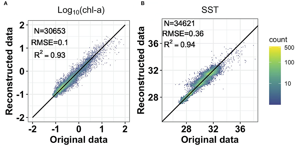
Figure 2. DINEOF validation between original and reconstructed data of chl-a (A) and SST (B).
EOF was used to examine the spatiotemporal variability of chl-a by extracting the common patterns. The results are shown by leading modes of spatial EOF and principal component (PC) of time series in each mode. EOF can be easily calculated using SVD by decomposition of matrix X that contains m × n dimensions; where each row (m) in the matrix represents data at one time, while each column (n) represents time-series data in one pixel (Brörnsson and Venegas, 1997). To avoid the non-normal distribution of chl-a data, the data were log10-transformed before applying EOF and the mean of pixels was removed.
The impact of ENSO on chl-a in each season was also studied using EOF. Three-month running mean was applied to chl-a data to reduce high-frequency noise in each pixel. The data were averaged seasonally and then separated into three data sets NEM (2002–2020), NON (2003–2021), and SWM (2002–2020). The seasonal climatological chl-a in each season was removed in all datasets. The results can describe year-to-year variation of chl-a in each season (Iskandar et al., 2017).
The relationship between chl-a and environmental parameters was investigated using Pearson correlations. Area-averaged time series data of chl-a and all parameters in each small area were computed.
Results
Seasonal distribution of surface chl-a and environmental parameters
Surface chl-a
The 18-year seasonal climatological chl-a data are presented in Figures 3A–C. Chl-a in the GoT near the coastal area and the river mouths were high throughout the year, especially in the UGoT and Rach Gia Bay, Vietnam in all seasons. During the NEM season (November to February), chl-a was higher than in other seasons almost throughout the area (Figure 3A). High chl-a near Ca Mau Cape was clearly observed with offshore expansion to the middle of the GoT mouth. Meanwhile, chl-a in the UGoT was clearly higher on the western coast than on the eastern coast. Chl-a was consistently high (> 1 mg m−3) along the southern coast from the GoT mouth to the inside of the GoT. During the NON season (March to May), chl-a was low in both offshore and coastal areas. The area with chl-a > 0.5 mg m−3 corresponded with the area shallower than 40 m (Figure 3B). Low chl-a area (< 0.1 mg m−3) appeared from the SCS to the central GoT. The offshore bloom area near Ca Mau Cape became smaller with a lower concentration than during NEM, and chl-a in the UGoT was high (> 3 mg m−3) only in the head of the UGoT. In the SWM (June to October), chl-a along the eastern coast was higher than on the western and the southern coasts. Low chl-a area (< 0.1 mg m−3) decreased in central GoT and appeared near the southern coast. High chl-a area in the UGoT was obviously extended to the south (Figure 3C). In addition, a curve of high chl-a patch (> 0.2 mg m−3) was observed along the GoT mouth.
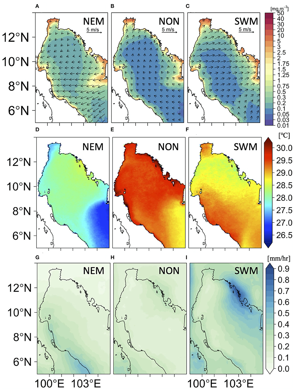
Figure 3. Seasonal climatology of chl-a with sea surface wind (A–C), SST (D–F), and precipitation (G–I).
Seasonal variation of environmental parameters
Seasonal wind (Figures 3A–C), SST (Figures 3D–F), and precipitation (Figures 3G–I) showed clear differences in each season. During NEM, strong northeast wind (5–6 m/s) from the SCS flowed across the GoT mouth, while weak northeast wind was observed in the upper part of the GoT with a magnitude of 1–2 m/s (Figure 3A). Meanwhile, the easterly wind was dominated in the central part with a magnitude of 2–3 m/s. During this time, cold water from the SCS was advected to the inside of the GoT near Ca Mau Cape by the northeast wind. Low SST was also found in the UGoT, associated with northeasterly wind. SST along the southern and the eastern coasts were warmer than offshore. The NEM brings moisture from the SCS region to this area and produced high precipitation along the southern coast (Figure 3G).
During NON or a summer season in this area, wind from the SCS flowed westward to the inside of the GoT and changed direction to northward in the northern part (Figure 3B) with a stronger magnitude (2–3 m/s). In this season, SST generally became high almost throughout the area especially near the coastal region (31°C), while SST offshore was lower. The lowest SST was found in the east of Ca Mau Cape (Figure 3E). Precipitation and river discharge over the GoT were lowest during this time (Figure 3H). The spatial distribution in NON showed slightly high precipitation over the eastern coast than the southern and the western coasts.
During SWM, wind over the UGoT and the GoT mouth flowed from the southwest with low magnitude (1–2 m/s). The westerly wind was clearly observed over the central GoT and the northern part with a high magnitude (3–5 m/s). The spatial distribution of SST showed a similar pattern with the NON season, except for lower SST in the northern part and along the east coast. In the meanwhile, high precipitation was clearly observed over the eastern coast (Figure 3I).
Spatiotemporal variability of chl-a
Section Surface chl-a and Figures 3A–C simply showed seasonal distributions of chl-a in the GoT. We then further investigated the dominant patterns of spatial and temporal variability of chl-a using EOF. The common patterns of chl-a variability were captured in EOFs while the corresponding temporal variabilities were shown in the PCs time series. The positive/negative areas in EOF with positive/negative PC reflected a positive chl-a anomaly from the mean. In contrast, the positive/negative areas in EOF with negative/positive PC indicated a negative chl-a anomaly.
The first three dominant modes accounted for 57.32% of the total variance, and clearly explained the seasonal variation of chl-a. The first mode (Figure 4A) explained 40.49% of the total variance. Most of the areas were characterized by a positive phase with a high magnitude near the Ca Mau Cape and along the southern coast, while the opposite phase was observed on the eastern coast, especially east of the UGoT. The corresponding temporal variation revealed the seasonal cycle by a peak during the NEM and troughs from NON to SWM by the lowest from April to May (Figure 4D). The second mode is accounted for 11.64% of the total variance. The positive areas were observed near the GoT mouth, the eastern coast, and the eastern part of the UGoT (Figure 4B). In addition, the area near Ca Mau Cape reflected the opposite phase of variation as same as near the southern coast. The positive phase of this mode was found in SWM with the highest in mid-SWM, and the negative phase occurred from November to May with the lowest in April (Figure 4E). The first two modes have shown a clear difference in the seasonal variation of chl-a during NEM and SWM, respectively, and including NON which showed a negative phase in both two modes. The third mode explained 5.19% of the total variance and described the variability in the eastern and western to southern coasts (Figure 4C). The areas with the highest positive variability were found on the western coast from UGoT to 10 degrees north, river mouth along the southern coast, and near Ca Mau Cape. The opposite phase was found in the middle gulf by stretches in the north-south direction. The time series showed a peak only 3 months in a year, from October to December with the highest in November (Figure 4F) and the lowest in February. This mode indicated the variability during transition periods from SWM to NEM and NEM to NON. The first three modes of EOF clearly explained the seasonal variation of chl-a in this area.
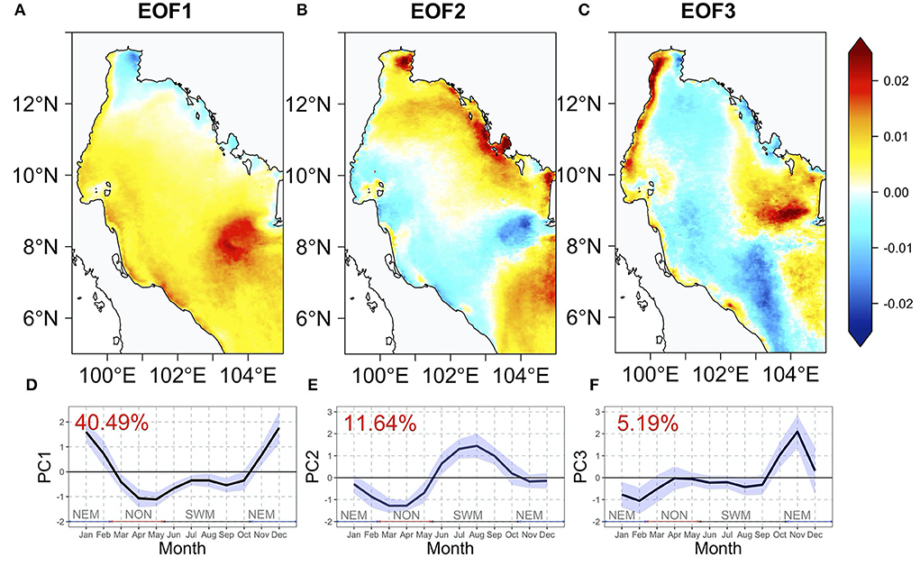
Figure 4. Spatial pattern of EOFs (A–C) and PCs monthly composite (D–F) of the first three modes for chl-a. The black lines and shaded areas in (D–F) indicate monthly means and standard deviations, respectively, of the PC time series from 2002 to 2020.
Detail of chl-a variability and environmental parameters
Spatial components of three EOFs were used to delineate the area of chl-a variations by combining all EOFs. The overlapped areas by three modes with signals (positive and negative) were classified to understand more detail about chl-a variability. Among the eight temporal variations, six patterns covered most of the GoT. The correlation analysis was also applied between the time series of chl-a and environmental parameters in each area to investigate their relationship. Figure 5A demonstrates six areas of dominant chl-a patterns, and seasonal and interannual variations of chl-a (Figures 5B–M).
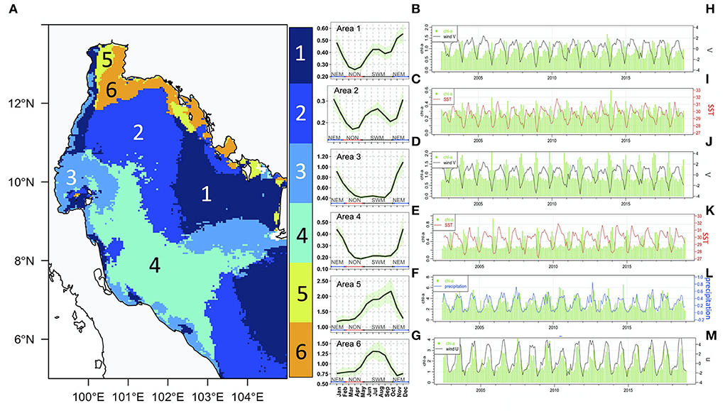
Figure 5. Areas of chl-a variability (A), monthly climatological chl-a (black line) with standard deviations (shade) in each area (B–G), and interannual variability of chl-a with the strongest correlated environmental parameter (H–M).
Area 1 reflects a positive phase in all EOF modes by covering the northwest and the south of Ca Mau Cape. The small areas were also found along the western UGoT and near the river mouths on the southern coast. Chl-a was lowest during NON (0.25 mg m−3) and increased from SWM to NEM, a small trough was found from September to October. Meridional wind component performs strongest relationship with chl-a (r = −0.64) (Figure 5H). Moreover, chl-a was negatively correlated with SST, and zonal wind (r = −0.52, −0.16, respectively), and positively correlated with wind speed and precipitation (r = 0.40, 0.17, respectively) (Table 1).
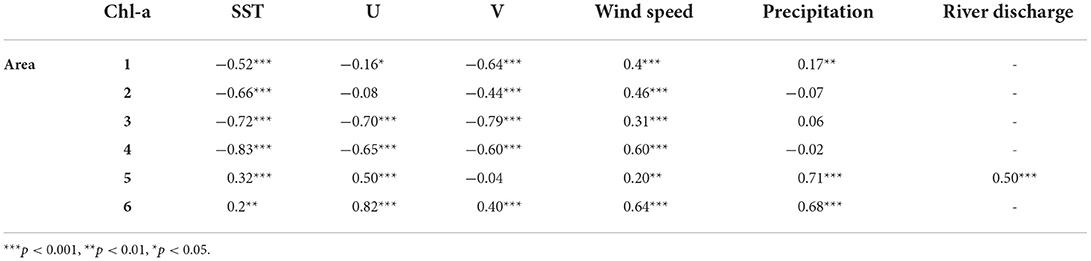
Table 1. Correlation coefficients between chl-a and environmental parameters.
Area 2 was determined by positive areas in the first two modes with a negative area in the third mode. This area covered the central GoT and near the south of the GoT mouth. The temporal variation of chl-a in this area was high in SWM and NEM by highest in January, and low during monsoon transitional periods. Chl-a in this area was negatively correlated with SST and meridional wind. Only wind speed showed a positive relationship with chl-a in this area (Table 1). The correlation between chl-a and SST was highest (r = −0.66; Figure 5I), followed by the relationship to wind speed (r = 0.46) and meridional wind (r = −0.44).
Area 3 is covered from the western to the southern coast and near Ca Mau Cape. This area was classified by positive areas in the first and the third modes, and a negative area in the second mode. Chl-a in Area 3 showed only one peak during NEM and a trough from NON to SWM. Chl-a was related to all parameters except precipitation. Meridional and zonal wind components and SST showed a strong negative correlation with r = −0.79, −0.70, and 0.72, respectively, while wind speed was positively correlated with chl-a with r = 0.31 (Table 1).
Area 4 dominated the offshore southern part. This area was created by a positive area in the first mode, and negative areas in the second and the third modes. Area 4 presented similar temporal patterns to Area 3, but the chl-a increased 1 month later. All parameters except precipitation were significantly correlated with chl-a. SST, meridional, and zonal wind components showed negative correlation, while wind speed was positively correlated with chl-a. SST in this area showed a higher correlation with r = 0.83 (Figure 5K).
The central UGoT and the eastern coast were defined as Area 5. This area was determined by the negative area in the first mode and the positive areas in the second and the third modes, respectively. The temporal variation revealed high chl-a during SWM by peaked in October and rapidly decreased in November. Chl-a was positively correlated with precipitation with r = 0.71 and followed by river discharge, zonal wind, SST, and wind speed (r = 0.50, 0.50, 0.32, 0.20, respectively).
Area 6 covered the eastern coast of the UGoT and along the eastern coast of the GoT. This area is delineated by a positive area from the second mode and negative areas in the first and the third modes. High chl-a was found only from June to September. All parameters were positively correlated with chl-a. The correlation of chl-a was highest with zonal wind (r = 0.82; Figure 5M), followed by precipitation, wind speed, meridional wind component, and SST (r = 0.68, 0.64, 0.40, and 0.20, respectively) (Table 1). The summary of chl-a in each area is shown in Table 2.
Table 2. Summary of chl-a variability in the GoT.
Influence of ENSO on chl-a and environmental parameters
The impact of ENSO on chl-a in each season was investigated using EOF based on seasonal anomaly data. The results indicated a year-by-year variation of chl-a in each season. In this part, we focus only on the first mode of each season due to account for dominant variation in terms of interannual variation. The first mode of NEM accounted for 18.64% of the total variance. The positive areas were located at the UGoT and Ca Mau Cape and expanded to the western part of the Ca Mau tip. The negative areas were found offshore, along the western coast, and near the GoT mouth (Figure 6A). The positive years were 2002, 2005, 2006, 2008, 2009, 2011, 2012, 2014, 2015, and 2018 while the negative years were 2003, 2004, 2007, 2010, 2013, 2016, 2017, and 2020 (Figure 6D).
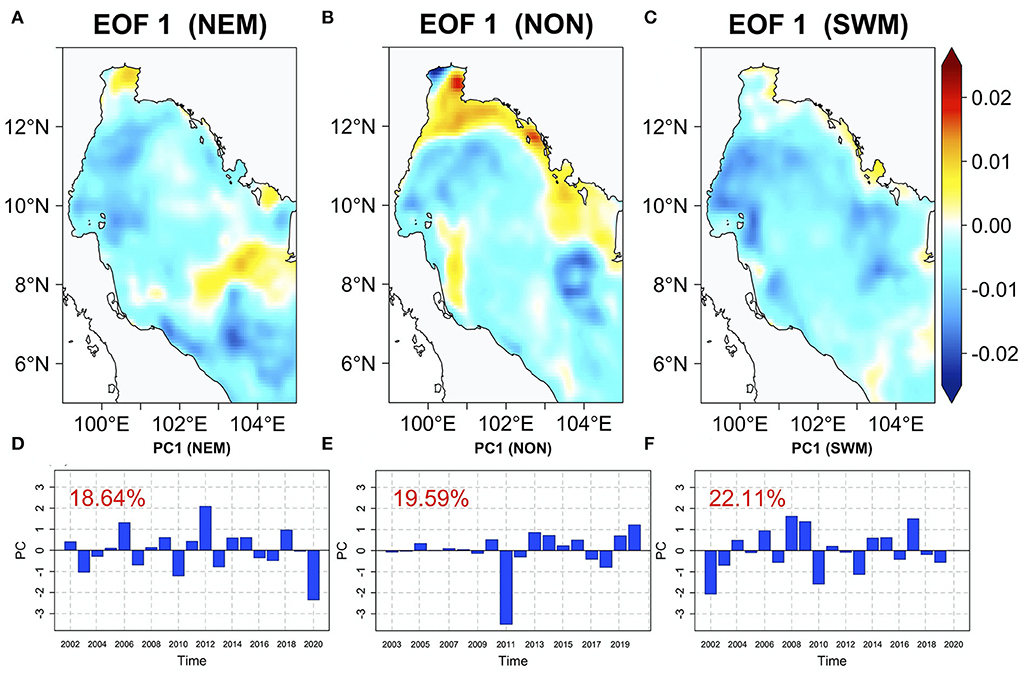
Figure 6. The first EOF mode of chl-a in each season (A–C) and PCs (D–F).
The first mode of NON explained 19.59% of the total variance. During NON, strong variations of chl-a areas were found near the UGoT, the shallow area along the eastern coast, and near Ca Mau Cape. The positive areas were in the eastern UGoT, between the UGoT and the GoT, and along the eastern and southern coasts. The large negative areas were in the western UGoT and Ca Mau Cape; moreover, the offshore area showed lower variation with a negative signal (Figure 6B). The time series during NON indicated a large negative event (LA) during 2011, while the positive years were 2005, 2007, 2008, 2010, 2013–2016, and 2019–2020 (Figure 6E).
For SWM, the first mode described 22.11% of the total variance, chl-a in the whole area especially along the western coast and the eastern part of the offshore area showed negative values. The positive areas were observed near the eastern UGoT and along the eastern coast at a short distance from the coast (Figure 6C). The positive years were 2004, 2006, 2008–2009, 2012, 2014–2015, 2017, and 2020 while the negative years were 2002–2003, 2005, 2007, 2010, 2013, 2016, and 2018–2019 (Figure 6F).
The relationship between PC in each season with MEI was investigated (Figure 7A). The PCs from NEM and NON were significantly positively correlated with MEI. The correlation coefficients during NEM and NON were 0.53 and 0.64, respectively. Meanwhile, the PC of SWM was not correlated with MEI. We also investigated the relationship between PCs and Dipole Mode Index (DMI), but the results showed no correlation between DMI and PCs in all seasons (Figure 7B).
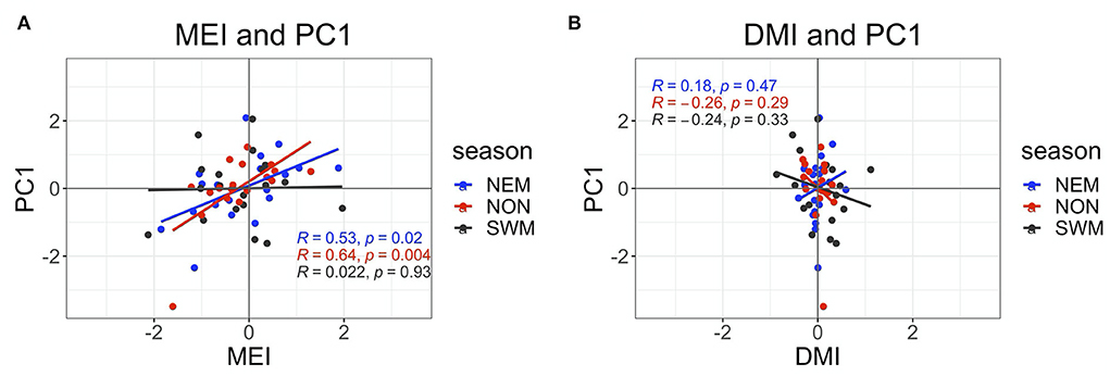
Figure 7. Scatter plots between seasonal averaged MEI (A) and DMI (B) with PC1 of all seasons during 2002–2020.
To explain the variability of chl-a under EN/LN events, the seasonal anomalous environmental parameters were composited under EN/LN events. Here, we showed only two seasons (NEM and NON) because the PC of SWM was not correlated with MEI. The anomalies of environmental parameters were similar in both seasons. In general, SST was high/low during EN/LN, almost throughout the area (Figures 8A,B). Under EN condition, SST anomaly in NON was higher than NEM (Figure 9A). Under the LN condition, the distribution showed a different pattern between NEM and NON (Figures 8B, 9B). SST during NEM was lower than normal in the northern part while SST in the lower GoT was higher than normal, especially in the GoT mouth. For SST anomaly in NON under LN condition was lower in all the areas, especially near Ca Mau Cape (Figure 9B) where the cold tongue was found in normal condition.
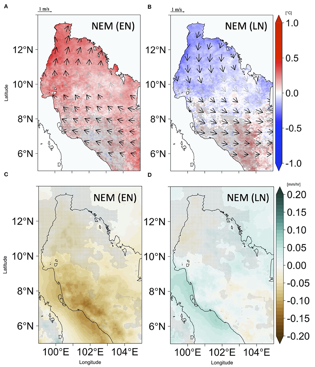
Figure 8. SST and wind anomalies under EN (A) and LN (B) with precipitation anomaly under EN (C) and LN (D) during NEM. The gray vectors and dots indicate the non-significant level (p > 0.05) of correlation between the parameter and MEI.
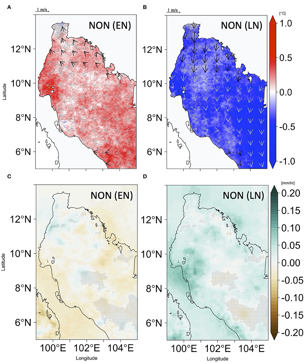
Figure 9. SST and wind anomalies under EN (A) and LN (B) with precipitation anomaly under EN (C) and LN (D) during NON. The gray vectors and dots indicate the non-significant level (p > 0.05) of correlation between the parameter and MEI.
In general, wind anomalies showed a similar pattern in both NEM and NON. Westward and northwestward wind anomalies were found under EN; in contrast, south-eastward wind anomalies were found under LN (Figures 8A,B, 9A,B). Under EN, wind anomaly near the GoT mouth was westward and induced stronger wind blowing into the GoT than normal conditions in both NEM and NON. Over the northern area during NEM, wind anomaly under EN was north-northwestward indicating weaker wind condition. The north-northwestward wind anomaly over the northern area remained to NON season, and it supported the NON wind leading to stronger wind during EN. On the other hand, south-eastward wind anomalies during LN in the northern part indicated stronger wind during NEM and weaker wind during NON. Wind anomaly near the GoT mouth indicated weaker wind blowing into the GoT in both NEM and NON during LN.
The precipitation anomalies clearly showed lower and higher than normal under EN and LN, respectively (Figures 8C,D, 9C,D). During NEM, precipitation was lower/higher than normal under EN/LN condition in the GoT, especially along the southern coast. Meanwhile, precipitation in NON was low/high almost throughout the area except in some areas under EN/LN.
Discussion
In this study, the influences of tropical monsoon and ENSO on chl-a in the GoT have been examined using chl-a from MODIS data. Satellite-derived chl-a data are useful information to estimate phytoplankton at the surface of the ocean, but one of the major problems is cloud coverage. In this study, the missing data in both temporal and spatial gaps were reconstructed using the DINEOF method (Beckers and Rixen, 2003; Alvera-Azcárate et al., 2005). The reconstructed chl-a and SST data from DINEOF were verified with the original data which had been masked before applying DINEOF. Reconstructed chl-a showed good agreement with the original data for both chl-a and SST, respectively (Figure 2).
Seasonal variability of surface chl-a was revealed by long-term composite and EOF analysis. The regional difference in seasonal variability of chl-a in the GoT was also shown by combining the results from EOFs. The GoT was separated into six dominant areas which showed different temporal variations of chl-a. These results gave a more detailed structure of chl-a variability related to monsoons, which have never been reported before. The four areas of chl-a variability covered the eastern coast (Area 1, 5, 6) as well as western to southern coasts (Area 1, 3), and the other two areas dominated in the offshore area (Area 2, 4). The correlation between chl-a and environmental parameters within six areas showed that chl-a in the coastal (Area 1, 3, 5, 6) and offshore (Area 2, 4) areas responded to different environmental parameters. The relationships between chl-a and environmental parameters may indicate the mechanisms that occurred (Waite and Mueter, 2013; Moradi and Moradi, 2020). It suggested that different mechanisms existed and controlled chl-a variation in the coastal and offshore areas.
The mechanisms related to physical parameters are discussed separately between coastal and offshore areas in the next sections. Meanwhile, the influence of ENSO is discussed in each season.
The coastal areas
In general, chl-a in the coastal areas are significantly correlated with precipitation, river discharge, and wind (Table 1). Nutrient loading and advection by ocean current are expected to be the major processes that controlled chl-a in the coastal areas especially UGoT (Buranapratheprat et al., 2009; Luang-on et al., 2021).
Along the southern coast, temporal variation of chl-a near the river mouths (Area 1) was similar to the time change of precipitation and associated nutrient loading that was usually low in NON then increased in SWM with peaked in NEM (Wattayakorn et al., 2000, 2001). Meanwhile, chl-a areas far from estuaries along the southern coast (Area 3) were high only NEM (Figure 5D). The variability of chl-a in these areas was captured by the third EOF mode (Figure 4C), and the influences of river discharge and northeast wind were revealed. High river discharges from late SWM to NEM which contain nutrients may be transported outside the estuary.
On the western coast, Sripoonpan and Saramul (2021) pointed out favorable upwelling areas located on the western coast during SWM based on Ekman transport and SST upwelling indexes. High chl-a is expected; however, chl-a near the western coast (Area 3) was not high during SWM (Figures 5A,D). This may be due to the westerly wind along the western coast was not strong enough, together with shallow topography (< 20 meters) and bottom friction, resulting in unfavorable upwelling development. Meanwhile, chl-a at far away from the western coast (Area 1) where bottom topography > 20 m was increased during SWM (Figures 5A,B) which may be a response to upwelling condition. During late SWM, high river discharges in October from the UGoT were transported by surface circulation to this area resulting in high chl-a during this time (Buranapratheprat and Bunpapong, 1998; Yu et al., 2018).
Previous studies of the UGoT by numerical models, cruise observations, and satellite observations have reported that low salinity water mass with high nutrients and high chl-a along the western/eastern coast corresponded to anticlockwise/clockwise circulation that developed during NEM/SWM season (Buranapratheprat et al., 2002, 2021; Yu et al., 2018; Luang-on et al., 2021; Morimoto et al., 2021). Our results showed that chl-a was high in early SWM in all the UGoT (Area 1, 3, 5, 6), and then peaked in mid-SWM in the eastern UGoT, corresponding to a strong eastward wind component. The northeast wind became stronger resulting in high chl-a in the central UGoT (Area 5) and the western UGoT (Area 1, 3). Our results also showed that chl-a in the UGoT can be transported to the south of the UGoT and the western coast during NEM, but during SWM, chl-a cannot be transported to the eastern GoT (Figure 4B). The second and the third EOF have highlighted the influence of freshwater from the UGoT in the eastern and the western UGoT during SWM and the transition period, respectively (Figures 4B,C). Furthermore, chl-a in the central UGoT showed a positive relationship with precipitation and river discharge which was similar to other tropical coastal seas, such as the Indonesian Sea (Longhurst, 2007; Iskandar et al., 2017; Chang et al., 2019; Siswanto et al., 2020; Wirasatriya et al., 2021).
Along the northern and the eastern coasts (Area 5, 6), high chl-a showed a positive relationship with zonal wind and precipitation. SWM induced strong westerly wind near the coast and high precipitation in this area resulting in the highest nutrient fluxes exported in this season (Kan-atireklap et al., 2017; Meesub et al., 2021). Although Huynh et al. (2020) suggested that river discharge associated with the southwest wind may contribute to high chl-a on the eastern coast. It should be noted that chl-a along the eastern coast responded to local freshwater rather than the impact of freshwater from the major rivers. Zonal wind also contributed to water mixing as shown by low SST along the eastern coast during SWM (Figure 3F). During NEM precipitation on the eastern coast was lowest, and the northeast wind was not strong enough to induce upwelling, due to the effect from the Cardamom Mountain along the eastern coast that blocks the northeast wind (Li et al., 2014).
Chl-a in the west of Ca Mau Cape (Area 1) peaked during NEM which may be related to the influence of discharge that was captured by the third EOF mode (Figure 4C). At the west of Ca Mau Cape where there is no large river, Mekong River discharge headed to the SCS, and high nutrients from untreated water from agricultural and urban areas in the canal system (Minh et al., 2019, 2020) may be drained directly to the GoT via dug-canal networks along Mekong delta. This was similar to the UGoT area, where the canal networks may contribute to the nutrient supplies (Luang-on et al., 2021).
Offshore bloom near Ca Mau Cape was found during NEM due to surface current flew into the GoT from the Vietnam coast (Huynh et al., 2020). The current may bring discharged water from the Mekong River to this area and contribute to the offshore bloom (Tang et al., 2006). Previous studies by Tang et al. (2006) revealed that high turbid areas were located near Ca Mau Cape and that the turbidity was higher during NEM than SWM. Thus, satellite chl-a in those regions can be also overestimated by the sediment loads.
In this study, we have clearly separated the areas that were influenced by precipitation, river discharge, and wind. We have emphasized the influence of seasonal precipitation, river discharge, and seasonal wind on chl-a in each part of the GoT coast (Areas 1, 3, 5, and 6). Moreover, high chl-a from the UGoT area could be carried to the GoT, and this may be important in supporting marine resources. These suggested that chl-a along the coast is controlled by the interaction between nutrient loading and advection from ocean circulation.
The offshore areas
Chl-a in the offshore areas have two different patterns; (1) high chl-a during NEM and SWM (Area 2) in the northern region, and (2) the chl-a peaked only during NEM (Area 4) in the southern region. The observation in 2013 by SEAFDEC cruise revealed that high salinity with low-temperature water mass in the deep layer contains higher nutrients than the surface (Sompongchaiyakul et al., 2013). In this area, chl-a was negatively correlated with SST and positively correlated with wind speed. The vertical mixing was previously expected to be a major mechanism that controlled chl-a variability in this area (Tang et al., 2006; Huynh et al., 2020), and also the cyclonic eddy and coastal upwelling were then reported by Guo et al. (2021) and Sripoonpan and Saramul (2021), respectively. The vertical-mixing process and upwelling are known to significantly support nutrients from the subsurface to the surface. Furthermore, the vertical-mixing process may also break pycnocline and bring phytoplankton from the subsurface chlorophyll maximum layer to the surface (Moradi and Moradi, 2020).
During NEM, the cyclonic circulation was developed in the northern GoT over Area 2 during weak and moderate northeast wind (November to December), the cyclonic circulation then disappeared during strong northeast wind (January to February) (Guo et al., 2021). This cyclonic circulation may be induced upwelling in this area and may contribute to high chl-a during NEM. Meanwhile, over Area 4 high chl-a may be induced by the water mixing developed by surface cooling and strong wind during NEM suggested by Yanagi et al. (2001).
Strong surface heating during NON enhanced water stratification and reduced vertical mixing throughout the area. Observation in 1995–1996 by SEAFDEC confirmed that strong stratification was developed during NON due to strong surface heating, weak wind, and SCS intrusion (Yanagi et al., 2001; Buranapratheprat et al., 2016). It corresponded to the low surface chl-a.
For SWM, strong westerly wind associated with the coastal boundary created clockwise circulation to the GoT mouth (Robinson, 1974; Buranapratheprat and Bunpapong, 1998; Higuchi et al., 2020; Sripoonpan and Saramul, 2021). Strong eastward wind and current in the northern GoT may create upwelling condition resulting in low sea surface height (Higuchi et al., 2020) and low SST (Figure 3F). This condition may occur in the area where the strong westerly wind is perpendicular to the topography. Our results from the second EOF mode also highlighted high chl-a near 12°N, occurring in the east-west direction along the slope of the region (30–40 m) during SWM. Sojisuporn et al. (2010) also reported that during SWM counterclockwise eddy over the northern region was developed. In the southern region (Area 4) during SWM, wind was not strong enough to create upwelling. Unfavorable mixing and upwelling were also indicated by warm SST and clockwise eddy (Sojisuporn et al., 2010; Sripoonpan and Saramul, 2021). In the GoT mouth, a band of high chl-a (> 0.2 mg m−3) was found in SWM due to the propagation of water mass from the upwelling area along the Peninsular Malaysia (Kok et al., 2015, 2017).
From our results, two areas in the offshore were distinguished. Based on the variability of chl-a and oceanographic conditions, the understanding of the mechanisms related on chl-a variability in the offshore area has been improved. We have pointed out that not only high chl-a induced by vertical mixing in the offshore region, but also upwelling may also exist in the GoT. Chl-a was high in NEM and SWM in the northern part (Area 2) as a result.
Influence of ENSO
It is also expected that large-scale phenomena, climate events, and associated abnormal conditions can change the variability of chl-a (Devred et al., 2007; Longhurst, 2007; Shalin et al., 2018). Thus, we applied EOF analysis to seasonal anomalies of chl-a data to investigate year-to-year variability in each season, and the environmental parameter anomalies were composited under EN and LN conditions. Our results showed that chl-a and environmental parameter anomalies varied oppositely for EN and LN. The patterns of chl-a anomaly were different in each season as well.
The correlations between PCs and MEI indicated that ENSO significantly influenced chl-a during NEM and NON (Figure 7). This is probably due to the influences of mature ENSO remained over the Southeast Asia mainland (Thirumalai et al., 2017) and the SCS region (Tang et al., 2011; Siswanto et al., 2017; Yu et al., 2019; Huynh et al., 2020) with 4–9 months.
During NEM under EN/LN condition, low/high chl-a anomaly in the offshore region coincided with high/low SST and weak/strong northeast wind in this study (Figures 8A,B). This is similar to the SCS open ocean, where the anticyclonic/cyclonic wind and circulation anomaly were developed (Kuo and Tseng, 2020) resulting in low/high chl-a during EN/LN (Siswanto et al., 2017; Yu et al., 2019; Huynh et al., 2020). The Ekman pumping anomalies during EN/LN in the offshore area of the GoT also indicated downwelling/upwelling but with weak magnitude (not shown). In the GoT, more weak/strong upwelling and water stratification/mixing were expected to occur during EN/LN in the northern and southern areas, respectively. In addition, low/high precipitation over the mainland Southeast Asia may contribute to low/high nutrient loading along the coast similar to the impact of ENSO on the Indonesian maritime continent (Siswanto et al., 2020). For chl-a near Ca Mau Cape during EN/LN could be explained by westward/eastward wind anomaly (Figures 8A,B) enhancing circulation of inward/outward to the GoT. This wind anomaly during EN/LN is connected with anticyclonic/cyclonic wind anomaly over the SCS (Siswanto et al., 2017; Kuo and Tseng, 2020). For the UGoT, high/low chl-a may be influenced by weak/strong northeast wind during EN/LN. Due to NEM, wind induced counterclockwise circulation and transported freshwater out of the UGoT. Weak/strong northeast wind may decrease/increase this outward transport of water from the UGoT resulting in high/low chl-a in the UGoT during EN/LN.
Similar to NEM, during NON under EN/LN condition, chl-a in the offshore area was low/high and coincided with high/low SST (Figure 9). Low/high chl-a in offshore areas may be related to water stratification/mixing developed by high/low heat flux (Yanagi et al., 2001; Wang et al., 2006; Buranapratheprat et al., 2016; Thirumalai et al., 2017). Although easterly wind anomaly during the EN increased strength of wind and more mixing was expected during NON, chl-a in the offshore was not responded to these modifications. This may be because strong heat and strong wind created deeper mixed layer with warm and less nutrient water mass, which is coincident with SCS intrusion in this season (Yanagi et al., 2001; Buranapratheprat et al., 2016). This situation is similar to the open ocean in SCS when thicker/thinner mixed layer depth was developed during EN/LN (Kuo and Tseng, 2020). On the other hand, strong/weak wind during EN/LN played an important role in water mixing in shallow areas near the northern coast where the topography is <20 m during NON. A previous study by Luang-on et al. (2021) also revealed that anomalous high/low chl-a in southeastern UGoT during NON responded to strong/weak NON wind under EN/LN condition. It was expected that wind-induced strong/weak mixing in the shallow region during EN/LN resulted in high/low chl-a in this season. Although the mechanism in shallow and offshore areas was the same, the shallower pycnocline in shallow water may be easily broken down.
High chl-a near the southern coast under EN during NON was observed by coinciding with easterly wind anomaly (Figures 6B, 9A). Sripoonpan and Saramul (2021) have reported that based on Ekman transport during NON in normal condition, the southern coast appeared to be in favorable upwelling condition, but SST did not indicate an upwelling condition. Strong NON wind during EN may increase stronger Ekman transport and lead to stronger upwelling along the coast than normal condition. SST anomaly under EN condition in this area remains unchanged but it was lower than the surrounding area (Figure 9A).
Our results also highlighted low/high offshore chl-a bloom near Ca Mau Cape during EN/LN. This variation may relate to low/high discharge from Mekong River under EN/LN condition (Räsänen and Kummu, 2013) associated with abnormal wind.
Besides ENSO, the GoT is also possibly affected by IOD. Luang-on et al. (2021) revealed that IOD also impacts the phytoplankton in the UGoT, but the impact is less than ENSO. However, our analysis could not capture the influence of IOD. This is probably because we applied EOF to the average seasonal anomalous data which straddled the peak of the IOD period (September to November) (Iskandar et al., 2017; Sari et al., 2018b).
In the GoT, the results from the observations by the NAGA expedition during 1959–1961 were used to indicate spawning areas and seasons of short mackerel (Faughn, 1963), which is one of the most important fishes in this area (Janetkitkosol et al., 2003). The spawning areas were considered based on the relationship between physical processes, zooplankton, larval, and juvenile forms of short mackerel (Faughn, 1963). However, the relationship between short mackerel and phytoplankton was not investigated. In this area, Chang Island on the eastern coast, the UGoT area, the western coast, Sumui Island (near Tapi River), and Pattani coast (the southern coast) are believed as spawning grounds of the short mackerel (Kongseng et al., 2020), and the population also migrates among these areas (Chomjurai et al., 1965; Kongseng et al., 2020). Our results showed the seasonal variation of chl-a, delineated marine ecosystem zones and the influence of ENSO. These results may help to improve understanding of fisheries dynamic in this region.
Conclusion
This study demonstrated the seasonal variability of surface chl-a in the GoT, as well as the influence of ENSO using reconstructed chl-a from MODIS data. Seasonal variation of chl-a was investigated by long-term composite data and EOF analysis. In general, high chl-a was found on the southwestern coast and Ca Mau Cape tip during NEM; and on the eastern coast, the UGoT, and near the mouth of GoT during SWM. Meanwhile, chl-a was low in both offshore and nearshore during NON. The contrasting chl-a patterns during NEM and SWM, as well as the low chl-a during NON were also emphasized by the first and second EOF modes. We delineated the GoT into six areas which have different seasonal variability of chl-a. Chl-a in the coastal area positively correlated with precipitation and river discharge indicating that chl-a may be enhanced by nutrient input. In addition, a positive correlation between chl-a and shoreward wind can be explained by transport and accumulation of chl-a. In the offshore area, chl-a may respond to the water column and upwelling conditions as reflected by its relationship to SST and wind. ENSO plays a crucial role in the variations of chl-a with interannual time scale. Its impacts were stronger during NEM and NON as compared with SWM. Low/high precipitation and river discharge during EN/LN may cause low/high nutrient input resulting in abnormal chl-a along the coastal area. In the offshore area, low/high chl-a during EN/LN was caused by weak/strong water mixing and upwelling conditions. Wind anomaly during EN/LN seems to enhance inward/outward circulation near the GoT mouth resulting in shifted high chl-a area near Ca Mau Cape. The results have expanded our understanding of phytoplankton variation and its mechanisms in the particular region of the GoT related to the tropical monsoon. This research has pointed out how the abnormal physical processes under ENSO can alter phytoplankton. Further investigation of the interaction mechanisms between physical and biological processes becomes necessary. Our future work will focus on the dynamics of physical and biological processes under different climate conditions using numerical models.
Data availability statement
Publicly available datasets were analyzed in this study. The chl-a and SST data can be found here: https://oceancolor.gsfc.nasa.gov. Wind components and wind speed are available at ECMWF website (https://www.ecmwf.int). Precipitation data are available at https://gpm.nasa.gov/data/imerg.
Author contributions
DL has performed analysis and wrote the manuscript. JL-o has supported the information about the data and analysis. AB and JI have supervised this work and revised the manuscript. All authors contributed to the article and approved the submitted version.
Acknowledgments
The authors would like to thank NASA Ocean Biology Processing Group, ECMWF, NASA/GSFC, NOAA Physical Sciences Laboratory, and Royal Irrigation Department, Thailand, for the data in this study. We also thank Assoc. Prof. Hidenori Aiki, Assoc. Prof. Hiroyuki Tomita, Assistant Prof. Yoshihisa Mino and lab members for their suggestions and discussions.
Conflict of interest
The authors declare that the research was conducted in the absence of any commercial or financial relationships that could be construed as a potential conflict of interest.
Publisher's note
All claims expressed in this article are solely those of the authors and do not necessarily represent those of their affiliated organizations, or those of the publisher, the editors and the reviewers. Any product that may be evaluated in this article, or claim that may be made by its manufacturer, is not guaranteed or endorsed by the publisher.
References
Alvera-Azcárate, A., Barth, A., Rixen, M., and Beckers, J. M. (2005). Reconstruction of incomplete oceanographic data sets using empirical orthogonal functions: application to the Adriatic Sea surface temperature. Ocean Model. 9, 325–346. doi: 10.1016/j.ocemod.2004.08.001
Beckers, J. M., and Rixen, M. (2003). EOF calculations and data filling from incomplete oceanographic datasets. J. Atmos. Ocean. Technol. 20, 1839–1856. doi: 10.1175/1520-0426(2003)020<1839:ECADFF>2.0.CO;2
Boonyapiwat, S. (1998). “Distribution, abundance and species composition of phytoplankton in the South China Sea, Area I: Gulf of Thailand and East Coast of Peninsular Malaysia.” in Proceedings of the First Technical Seminar on Marine Fishery Resources Survey in the South China Sea, Area I : Gulf of Thailand and East Coast of Peninsular Malaysia, 24–26 Nov. 1997 (SEAFDEC, Bangkok), 111–134.
Brörnsson, H., and Venegas, S.A. (1997). A Manual of EOF and SVD Analyses of Climatic Data. C2GCR Report No. 97-1. McGill University, Motreal, Canada.
Buranapratheprat, A., and Bunpapong, M. (1998). A two-dimensional hydrodynamic model for the Gulf of Thailand. In Proceeding of the IOC/WESTPAC Fourth International Scientific Symposium. 1, 469–478.
Buranapratheprat, A., Luadnakrob, P., Yanagi, T., Morimoto, A., and Qiao, F. (2016). The modification of water column conditions in the Gulf of Thailand by the influences of the South China Sea and monsoonal winds. Cont. Shelf Res. 118, 100–110. doi: 10.1016/j.csr.2016.02.016
Buranapratheprat, A., Morimoto, A., Phromkot, P., Mino, Y., and Gunbua, V. (2021). Eutrophication and hypoxia in the upper Gulf of Thailand. J. Oceanogr. 77, 831–841. doi: 10.1007/s10872-021-00609-2
Buranapratheprat, A., Niemann, K., Matsumura, S., and Yanagi, T. (2009). Meris imageries to investigate surface chlorophyll in the upper gulf of Thailand. Coast. Mar. Sci. 33, 22–28. doi: 10.15083/00040700
Buranapratheprat, A., Yanagi, T., and Sawangwong, P. (2002). Seasonal variations in circulation and salinity distributions in the upper Gulf of Thailand: Modeling approach. La Mer. 40, 147−155. Available online at: http://www.sfjo-lamer.org/la_mer/40-3/40-3-5.pdf
Chaiongkarn, P., and Sojisuporn, P. (2013). Characteristics of seasonal wind and wind-driven current in the Gulf of Thailand Bulletin of Earth Sciences of Thailand. Bull. Earth Sci. Thail. 5, 58–67. Available online at: https://ph01.tci-thaijo.org/index.php/bestjournal/article/view/246553
Chang, C. W. J., Hsu, H. H., Cheah, W., Tseng, W. L., and Jiang, L. C. (2019). Madden–Julian oscillation enhances phytoplankton biomass in the maritime continent. Sci. Rep. 9, 5421. doi: 10.1038/s41598-019-41889-5
Chomjurai, V., Somchaiwong, D., and Bunnag, R. (1965). “Growth and migration of chub mackerel, Rastrelliger neglectus, in the Gulf of Thailand.” in Reports on Mackerel Investigations 1963–1965. (Bangkok, Thailand: Marine Fisheries Laboratory, Division of Research and Investigations, Department of Fisheries), 28–114.
Devred, E., Sathyendranath, S., and Platt, T. (2007). Delineation of ecological provinces using ocean colour radiometry. Mari. Eco. Prog. Series. 346, 1–13. doi: 10.3354/meps07149
Faughn, J. L. (1963). Final Report of Naga Expedition. UC San Diego: Scripps Institution of Oceanography, 45. Available online at: https://escholarship.org/uc/item/6b05s9bp
Guo, J., Qu, D., Zhang, Z., Sangmanee, C., Chanthasiri, N., and Guo, B. (2021). Thermohaline conditions and circulation in the Gulf of Thailand during the northeast monsoon. Cont. Shelf Res. 225, 104487. doi: 10.1016/j.csr.2021.104487
Higuchi, M., Anongponyoskun, M., Phaksopa, J., and Onishi, H. (2020). Influence of monsoon-forced ekman transport on sea surface height in the gulf of thailand. Agric. Nat. Resour. 54, 205–210. doi: 10.34044/j.anres.2020.54.2.12
Huynh, H. N. T., Alvera-Azcárate, A., and Beckers, J. M. (2020). Analysis of surface chlorophyll a associated with sea surface temperature and surface wind in the South China Sea. Ocean Dynamics. 70, 139–161. doi: 10.1007/s10236-019-01308-9
Iskandar, I., Sari, Q. W., Setiabudiday, D., Yustian, I., and Monger, B. (2017). The distribution and variability of chlorophyll-a bloom in the southeastern tropical Indian ocean using empirical orthogonal function analysis. Biodiversitas. 18, 1546–1555. doi: 10.13057/biodiv/d180432
Janetkitkosol, W., Somchanakij, H., Eiamsa-ard, M., and Supongpan, M. (2003). “Strategic review of the fishery situation in Thailand, 915–956.” in Assessment, Management and Future Directions for Coastal Fisheries in Asian Countries, eds G. Silvestre, L. Garces, I. Stobutzki, M. Ahmed, R. A. Valmonte-Santos, C. Luna, et al. (WorldFish Center Conference Proceedings), 1120.
Kan-atireklap, S., Yuenyong, S., Phothong, K., Chotchuang, P., Buranapratheprat, A., and Kan-atireklap, S. (2017): Fluxes of dissolved inorganic nutrients total suspended solid at the phangrad river mouth, Rayong province during dry wet Seasons in 2015. Burapha Science Journal. 22, 500–509. Available online at: https://science.buu.ac.th/ojs246/index.php/sci/article/view/1732/1707
Kim, J. S., Xaiyaseng, P., Xiong, L., Yoon, S. K., and Lee, T. (2020). Remote sensing-based rainfall variability for warming and cooling in indo-pacific ocean with intentional statistical simulations. Remote Sens. 12, 1458. doi: 10.3390/rs12091458
Kirtphaiboon, S., Wongwises, P., Limsakul, A., Sooktawee, S., and Humphries, U. (2014). Rainfall variability over Thailand related to the El Niño-Southern Oscillation (ENSO). Journal of Sustainable Energy and Environment. 5, 37−42. Available online at: https://www.jseejournal.com/journal.php?id=21
Kok, P. H., Akhir, M. F., and Tangang, F. T. (2015). Thermal frontal zone along the east coast of Peninsular Malaysia. Cont. Shelf Res. 110. 1–15. doi: 10.1016/j.csr.2015.09.010
Kok, P. H., Akhir, M. F. M., Tangang, F., and Husain, M. L. (2017). Spatiotemporal trends in the southwest monsoon wind-driven upwelling in the southwestern part of the South China Sea. PLoS ONE. 12, e0171979. doi: 10.1371/journal.pone.0171979
Kongseng, S., Phoonsawat, R., and Swatdipong, A. (2020). Individual assignment and mixed-stock analysis of short mackerel (Rastrelliger brachysoma) in the Inner and Eastern Gulf of Thailand: Contrast migratory behavior among the fishery stocks. Fish. Res. 221, 105372. doi: 10.1016/j.fishres.2019.105372
Kuo, Y. C., and Tseng, Y. H. (2020). Impact of ENSO on the South China Sea during ENSO decaying winter–spring modeled by a regional coupled model (a new mesoscale perspective). Ocean Model. 152, 101655. doi: 10.1016/j.ocemod.2020.101655
Laonamsai, J., Ichiyanagi, K., and Kamdee, K. (2020). Geographic effects on stable isotopic composition of precipitation across Thailand. Isotopes Environ. Health Stud. 56, 111–121. doi: 10.1080/10256016.2020.1714607
Li, H., Liu, Y., Sun, C., Dong, Y., and Zhang, S. (2021). Satellite observation of the marine light-fishing and its dynamics in the South China Sea. J. Mar. Sci. Eng. 9, 1–29. doi: 10.3390/jmse9121394
Li, J., Zhang, R., Ling, Z., Bo, W., and Liu, Y. (2014). Effects of Cardamom Mountains on the formation of the winter warm pool in the gulf of Thailand. Cont. Shelf Res. 91, 211–219. doi: 10.1016/j.csr.2014.10.001
Li, Z., Cai, W., and Lin, X. (2016). Dynamics of changing impacts of tropical Indo-Pacific variability on Indian and Australian rainfall. Sci. Rep. 6, 1–7. doi: 10.1038/srep31767
Luang-on, J., Ishizaka, J., Buranapratheprat, A., Phaksopa, J., Goes, J. I., Kobayashi, H., et al. (2021). Seasonal and interannual variations of MODIS Aqua chlorophyll-a (2003–2017) in the Upper Gulf of Thailand influenced by Asian monsoons. J Oceanogr. 78, 209–228. doi: 10.1007/s10872-021-00625-2
Meesub, B., Buranapratheprat, A., Thaipichitburapa, P., Kan-atireklarp, S., and Kan-atireklarp, S. (2021). Fluxes of dissolved inorganic nutrients and suspended sediment at the Trat river mouth, Trat province in 2018. Burapha Sci. J. 26, 526–544. Available online at: https://science.buu.ac.th/ojs246/index.php/sci/article/view/3280
Minh, H. V. T., Avtar, R., Kumar, P., Le, K. N., Kurasaki, M., and Van Ty, T. (2020). Impact of rice intensification and urbanization on surface water quality in an giang using a statistical approach. Water. 12, 1710. doi: 10.3390/w12061710
Minh, H. V. T., Kurasaki, M., Van Ty, T., Tran, D. Q., Le, K. N., Avtar, R., et al. (2019). Effects of multi-dike protection systems on surface water quality in the Vietnamese Mekong Delta. Water. 11, 1010. doi: 10.3390/w11051010
Moradi, M., and Moradi, N. (2020). Correlation between concentrations of chlorophyll-a and satellite derived climatic factors in the Persian Gulf. Marine Pollution Bulletin. 161, 111728. doi: 10.1016/j.marpolbul.2020.111728
Morimoto, A., Mino, Y., Buranapratheprat, A., Kaneda, A., Tong-U-Dom, S., Sunthawanic, K., et al. (2021). Hypoxia in the Upper Gulf of Thailand: Hydrographic observations and modeling. J Oceanogr. 77, 859–877. doi: 10.1007/s10872-021-00616-3
Räsänen, T. A., and Kummu, M. (2013). Spatiotemporal influences of ENSO on precipitation and flood pulse in the Mekong River Basin. J. Hydrol. 476, 154–168. doi: 10.1016/j.jhydrol.2012.10.028
Robinson, M. K. (1974). The physical oceanography of the Gulf of Thailand, Naga Expedition; Bathythermograph (BT) temperature observations in the Timor sea, Naga Expedition, Cruise S11. Naga Report, 3. Available online at: https://escholarship.org/uc/item/4mf3d0b7
Saadon, M. N., Rojana-Anawat, P., and Snidvongs, A. (1998). “Physical Characteristics of Watermass in the South China Sea, Area I : Gulf of Thailand and East Coast of Peninsular Malaysia.” in Proceedings of the First Technical Seminar on Marine Fishery Resources Survey in the South China Sea, Area I: Gulf of Thailand and Peninsular Malaysia, 24-26 November 1997 (Bangkok, Thailand). Available online at: http://hdl.handle.net/20.500.12067/774
Sari, Q. W., Siswanto, E., Setiabudidaya, D., Yustian, I., and Iskandar, I. (2018a). Spatial and temporal variability of surface chlorophyll-a in the gulf of Tomini, Sulawesi, Indonesia. Biodiversitas. 19, 793–801. doi: 10.13057/biodiv/d190306
Sari, Q. W., Utari, P. A., Setiabudidaya, D., Yustian, I., Siswanto, E., and Iskandar, I. (2018b). Variability of surface chlorophyll-a distributions in the northwestern coast of Sumatra revealed by MODIS. Journal of Physics: Conference Series. 1080, 1–8. doi: 10.1088/1742-6596/1080/1/012045
SEAFDEC (2018). Fishery Statistical Bulletin of Southeast Asia 2016. Southeast Asian Fisheries Development Center, 143. Available online at: http://hdl.handle.net/20.500.12066/1818
Shalin, S., Samuelsen, A., Korosov, A., Menon, N., Backeberg, C., and Pettersson, L. H. (2018). Delineation of marine ecosystem zones in the northern Arabian Sea during winter. Biogeosciences. 15, 1395–1414. doi: 10.5194/bg-15-1395-2018
Shi, X., Liu, S., Fang, X., Qiao, S., Khokiattiwong, S., and Kornkanitnan, N. (2015). Distribution of clay minerals in surface sediments of the western Gulf of Thailand: Sources and transport patterns. J. Asian Earth Sci. 105, 390–398. doi: 10.1016/j.jseaes.2015.02.005
Simpson, J., and Sharples, J. (2012). Introduction to the Physical and Biological Oceanography of Shelf Seas. Cambridge: Cambridge University Press. doi: 10.1017/CBO9781139034098
Siswanto, E., Horii, T., Iskandar, I., Gaol, J. L., Setiawan, R. Y., and Susanto, R. D. (2020). Impacts of climate changes on the phytoplankton biomass of the Indonesian Maritime Continent. J. Mar. Syst. 212, 103451. doi: 10.1016/j.jmarsys.2020.103451
Siswanto, E., Ye, H., Yamazaki, D., and Tang, D. L. (2017). Detailed spatiotemporal impacts of El Niño on phytoplankton biomass in the South China Sea. J. Geophys. Res. Oceans. 122, 2709–2723. doi: 10.1002/2016JC012276
Sojisuporn, P., Morimoto, A., and Yanagi, T. (2010). Seasonal variation of sea surface current in the Gulf of Thailand. Coast. Mar. Sci. 34, 91–102. doi: 10.15083/00040677
Sompongchaiyakul, P., Uthaipan, K., and Bua-ngam, N. (2013). “Nutrients and Primary Productivity in the Gulf of Thailand.” In Proceedings of fisheries resources and marine environment survey results in the Central Gulf of Thailand (Bangkok, Thailand), 34-38. Available online at: http://hdl.handle.net/20.500.12067/1187
Sripoonpan, P., and Saramul, S. (2021). Coastal upwelling investigation in the gulf of Thailand using ekman transport and sea surface temperature upwelling indices. Eng. J. 25, 1–16. doi: 10.4186/ej.2021.25.7.1
Stansfield, K., and Garrett, C. (1997). Implications of the salt and heat budgets of the Gulf of Thailand. J. Mar. Res. 55, 935–963. doi: 10.1357/0022240973224184
Sukigara, C., Mino, Y., Yasuda, A., Morimoto, A., Buranapratheprat, A., and Ishizaka, J. (2021). Measurement of oxygen concentrations and oxygen consumption rates using an optical oxygen sensor, and its application in hypoxia-related research in highly eutrophic coastal regions. Cont. Shelf Res. 229, 104551. doi: 10.1016/j.csr.2021.104551
Tang, D. L., Kawamura, H., Shi, P., Takahashi, W., Guan, L., Shimada, T., et al. (2006). Seasonal phytoplankton blooms associated with monsoonal influences and coastal environments in the sea areas either side of the Indochina Peninsula. J. Geophys. Res. Biogeosci. 111, 1–9. doi: 10.1029/2005JG000050
Tang, S., Dong, Q., and Liu, F. (2011). Climate-driven chlorophyll-a concentration interannual variability in the South China Sea. Theor. Appl. Climatol. 103, 229–237. doi: 10.1007/s00704-010-0295-6
Thirumalai, K., DInezio, P. N., Okumura, Y., and Deser, C. (2017). Extreme temperatures in Southeast Asia caused by El Ninõ and worsened by global warming. Nat. Commun. 8, 15531. doi: 10.1038/ncomms15531
Vinayachandran, P. N., Francis, P. A., and Rao, S. A. (2009). Indian Ocean Dipole: Processes and impacts. Current Trends in Science. 46, 569–589. Available online at: https://www.ias.ac.in/public/Resources/Other_Publications/Overview/Current_Trends/569-589.pdf
Waite, J. N., and Mueter, F. J. (2013). Spatial and temporal variability of chlorophyll-a concentrations in the coastal Gulf of Alaska, 1998–2011, using cloud-free reconstructions of SeaWiFS and MODIS-Aqua data. Prog. Oceanogr. 116, 179–192. doi: 10.1016/j.pocean.2013.07.006
Wang, B., Huang, F., Wu, Z., Yang, J., Fu, X., and Kikuchi, K. (2009). Multi-scale climate variability of the South China Sea monsoon: a review. Dyn. Atmospheres Oceans. 47, 15–37. doi: 10.1016/j.dynatmoce.2008.09.004
Wang, C., Wang, W., Wang, D., and Wang, Q. (2006). Interannual variability of the South China Sea associated with El Niño. J. Geophys. Res. Oceans. 111, C003333. doi: 10.1029/2005JC003333
Wattayakorn, G., Ayukai, T., and Sojisuporn, P. (2000). Material transport and biogeochemical processes in Sawi Bay, southern Thailand. Phuket Marine Biological Center Special Publication. 22, 63–77. Available online at: https://www.dmcr.go.th/dmcr/fckupload/upload/147/file/SP_paper/2000%20Vol.22%207Wattayakorn.pdf
Wattayakorn, G., and Jaiboon, P. (2014). An sssessment of nutrient biogeochemical cycles in the Inner Gulf of Thailand. Eur. Chem. Bull. 3, 50–54. Available online at: https://epa.oszk.hu/02200/02286/00023/pdf/
Wattayakorn, G., Prapong, P., and Noichareon, D. (2001). Biogeochemical budgets and processes in Bandon Bay, Suratthani, Thailand. J. Sea Res. 46, 133–142. doi: 10.1016/S1385-1101(01)00077-6
Wirasatriya, A., Susanto, R. D., Setiawan, J. D., Ramdani, F., Iskandar, I., Jalil, A. R., et al. (2021). High chlorophyll-a areas along the western coast of south sulawesi-indonesia during the rainy season revealed by satellite data. Remote Sens. 13, 4833. doi: 10.3390/rs13234833
Wyrtki, K. (1961). Physical oceanography of the Southeast Asian waters. Scietific Resultas of Marine Investigations of the South China Sea and the Gulf of Thailand, 2. Available online at: https://escholarship.org/uc/item/49n9x3t4
Yanagi, T., Sachoemar, S. I., Takao, T., and Fujiwara, S. (2001). Seasonal variation of stratification in the gulf of Thailand. J. Oceanogr. 57, 461–470. doi: 10.1023/A:1021237721368
Yanagi, T., and Takao, T. (1998). Seasonal variation of three-dimensional circulations in the Gulf of Thailand. La Mer. 36, 43–55.
Yu, X., Guo, X., Morimoto, A., and Buranapratheprat, A. (2018). Simulation of river plume behaviors in a tropical region: Case study of the Upper Gulf of Thailand. Cont. Shelf Res. 153, 16–29. doi: 10.1016/j.csr.2017.12.007
Keywords: chlorophyll-a, monsoon, ENSO, Gulf of Thailand, tropical marine ecosystem
Citation: Leenawarat D, Luang-on J, Buranapratheprat A and Ishizaka J (2022) Influences of tropical monsoon and El Niño Southern Oscillations on surface chlorophyll-a variability in the Gulf of Thailand. Front. Clim. 4:936011. doi: 10.3389/fclim.2022.936011
Received: 04 May 2022; Accepted: 22 July 2022;
Published: 30 August 2022.
Edited by:
Iskhaq Iskandar, Sriwijaya University, IndonesiaReviewed by:
Tomoki Tozuka, The University of Tokyo, JapanRiza Setiawan, Gadjah Mada University, Indonesia
Copyright © 2022 Leenawarat, Luang-on, Buranapratheprat and Ishizaka. This is an open-access article distributed under the terms of the Creative Commons Attribution License (CC BY). The use, distribution or reproduction in other forums is permitted, provided the original author(s) and the copyright owner(s) are credited and that the original publication in this journal is cited, in accordance with accepted academic practice. No use, distribution or reproduction is permitted which does not comply with these terms.
*Correspondence: Dudsadee Leenawarat, ZHVkc2FkZWVsZWVAZ21haWwuY29t