A deep learning model for forecasting global monthly mean sea surface temperature anomalies

Sea surface temperature (SST) variability plays a key role in the global weather and climate system, with phenomena such as El Niño-Southern Oscillation (ENSO) regarded as a major source of interannual climate variability at the global scale. The ability to make long-range forecasts of SST variations and extreme marine heatwave events have potentially significant economic and societal benefits, especially in a warming climate. We have developed a deep learning time series prediction model (Unet-LSTM), based on more than 70 years (1950–2021) of ECMWF ERA5 monthly mean SST and 2-m air temperature data, to predict global 2-dimensional SSTs up to a 24-month lead. Model prediction skills are high in the equatorial and subtropical Pacific. We have assessed the ability of the model to predict SST anomalies in the Niño3.4 region, an ENSO index in the equatorial Pacific, and the Blob marine heatwave events in the northeast Pacific in detail. An assessment of the predictions of the 2019–2020 El Niño and the 2016–2017 and 2017–2018 La Niña show that the model has skill up to 18 months in advance. The prediction of the 2015–2016 extreme El Niño is less satisfactory, which suggests that subsurface ocean information may be crucial for the evolution of this event. Note that the model makes predictions of the 2-d monthly SST field and Nino 3.4 is just one region embedded in the global field. The model also shows long lead prediction skills for the northeast Pacific marine heatwave, the Blob. However, the prediction of the marine heatwaves in the southeast Indian Ocean, the Ningaloo Niño, shows a short lead prediction. These results indicate the significant potential of data-driven methods to yield long-range predictions of SST anomalies.

1. Introduction

Modes of inter-annual climate variability, such as El Niño-Southern Oscillation (ENSO) and Indian Ocean Dipole (IOD), are known to modulate the global sea surface temperature (SST) variability and the marine heatwave frequency, duration, and intensity (Saji and Yamagata, 2003; McPhaden et al., 2006; Holbrook et al., 2019). The climate modes influence SST variability locally and remotely, mostly through atmospheric teleconnection. Ocean circulation and large-scale oceanic waves also transmit climate signals to remote regions. SST variability and marine heatwave characteristics are also influenced by regional atmospheric and oceanic dynamics and coupled processes. The Blob marine heatwaves in the northeast Pacific during 2013–2015 and 2019 have been attributed to anomalous atmospheric pressure systems (Bond et al., 2015; Amaya et al., 2020). The teleconnection between the equatorial and northeast Pacific may be one of the key drivers to sustain the Blob warming over a multi-year period (Di Lorenzo and Mantua, 2016). Marine heatwaves off the west coast of Australia, the Ningaloo Niño, are due to both oceanic and atmospheric teleconnection from the equatorial Pacific (Feng et al., 2013) and the local air-sea coupling (Kataoka et al., 2014; Tozuka et al., 2021).

A timely forecast of global SST anomalies helps marine and terrestrial resource managers to mitigate potential risks from extreme climatic events. The prediction of ENSO and IOD events, indexed with equatorial SST anomalies in the equatorial regions, is important for forecasting rainfall, drought, and bushfire variability around the globe. Coupled ocean-atmosphere models have been used to forecast global SST variability. Most of the skill assessment has been for the inter-annual climate modes, with 3–4 season forecasting skills for ENSO and 1-2 seasons for IOD (Stockdale et al., 2011). Regional SST variability forecast has limited skills and is highly regionally dependent (e.g., Spillman and Smith, 2021), which is to some extent due to coupled ocean-atmosphere models not properly capturing important regional coupled processes driving the SST anomalies (e.g., Doi et al., 2013).

Coupled model outputs have also been used to train machine learning (ML) models to assess the predictability of climate modes. A convolutional neural network (CNN) model has been proven to have a long-lead prediction skill (up to 18-month) for December-February Niño3.4 SST—an index for ENSO variability, trained by SST, and upper ocean heat content anomalies from coupled models (Ham et al., 2019). Similarly, an artificial neural network model has been trained to forecast the SST variations at the peak season of the IOD events (Ratnam et al., 2020). Rojo Hernández et al. (2020) used a nonhomogeneous hidden Markov model to achieve superior prediction skills of Nino3.4 SST variability compared to dynamic forecasting models at up to a 9-month lead time. Given the phase-locking characteristics of the climate modes, these models aim to make single-season predictions, and for a single climate index. SST variability outside the ENSO and IOD regions also show some seasonal phase-locking, such as the Ningaloo Niño marine heatwaves are phase-locked to austral summer (Kataoka et al., 2014; Feng et al., 2015).

Complex spatio-temporal variations of the climate modes have been recognized, such as the complexity in ENSO dynamics and predictability (Timmermann et al., 2018). During the 2009-2010 El Niño, the peak SST warming occurred in the central Pacific so that the event is being classified as a central Pacific El Niño, as compared with the more traditional 2015–2016 El Niño when the extreme warming was more located in the eastern equatorial Pacific. Marine heatwaves across the global ocean have diverse spatial variability and are to some extent not tightly phase-locked with seasons (Gupta et al., 2020). For example, the Blob marine heatwave can occur in different seasons (Amaya et al., 2020), whereas the Ningaloo Niño has substantial spatial variations among different events (Feng et al., 2015). An all-season CNN model has been proposed, arguing that it would overcome some arbitrary fluctuations in the predictions at different lead times. Still, the prediction aims for a single index, the Niño3.4 (Ham et al., 2021). Thus, it is important to explore ML models which can predict the full seasonal cycle and the spatial patterns of SST anomalies. It is also crucial for the model to take into account the steady SST increase under the influence of anthropogenic global warming.

In this study, we propose a new deep learning modeling framework to forecast monthly global SST, using an Unet-LSTM convolutional encoder-decoder neural network (Taylor et al., 2021), which has been proven to have better prediction skills while using fewer parameters, compared with other deep learning architectures (Larraondo et al., 2019). We train the model with observed (reanalysis) SST and surface air temperature data over the past 7 decades to demonstrate potential long lead predictions for SST variability in the tropical-subtropical oceans. We present the methodology and examine the predictability of SST anomalies in the equatorial Pacific and the Blob region in detail, whereas a full exploration of the machine learning model and SST predictability will be presented in the future work.

2. Materials and methods

2.1. Dataset

The ERA5 reanalysis data set (Hersbach et al., 2020) provides monthly estimates, currently commencing in 1979, of many atmospheric, land, and oceanic variables at global scale with a spatial resolution of 0.25°, ≈ 30 km. An ERA5 preliminary analysis commencing in 1950 and covering the period up to December 1978 is also available. The ERA5 data set includes surface variables, including SST, and atmospheric variables computed on 137 levels to a height of 80 km. ERA5 dataset was created by combining a comprehensive set of historical meteorological observations with a sophisticated data assimilation and modeling workflow developed by ECMWF. Most reanalysis products use gridded SST observations as their lower boundary forcing. Based on an assessment of the ERA5 surface data, it is suggested that the reanalysis skill for surface temperature is compatible with other reanalysis products (Simmons et al., 2021). We use a replica of the ERA5 data set available at the National Computational Infrastructure (NCI) (NCI, 2020). ERA5 data can also be obtained on request from ECMWF's meteorological data archive and retrieval system (MARS).

Our experiments use SST (ERA5 label “sst”) and 2-m atmospheric temperature (ERA5 label “t2m”) variables drawn from the ERA5 data set. 2-D convolutions require a full 2-D grid when modeling the oceans at the global scale. The 2-meter atmospheric temperature data was used only over the land surface in order to complete a global grid of data for use with the 2-D convolutional model layers. As both the SST and 2-metre atmospheric temperature data are from the same ERA5 reanalysis data set they are physically consistent within the limits of the reanalysis system. We selected the t2m data in order to minimize the impact of the transition between the ocean and continents. The t2m values are driven by different processes over the continent; however, we are using an ML model that is predicting SSTs by adjusting the weights in the model layers. The t2m data over the continents contributes no information to the prediction of SSTs will have weights that are zero, or close to zero, and where the t2m data contributes information the weights will be set above zero. The approach we have adopted leads to improved prediction of SSTs at the continental margins compared, for example, to setting all values over the continents to a constant in our earlier experiments. Other approaches to solving this problem could be investigated, especially where the focus is on SSTs near the coastal margins; however, it does not have a significant impact on the predicted SSTs beyond the coastal margins.

Figure 1 provides an example of the ERA5 monthly mean SST, 2-meter air temperatures and the combined temperatures for March 2010. We start with the full global data set with latitude and longitude dimensions of [720,1440]. The temporal domain data span January 1950 until May 2021, with a temporal resolution of 1 month, a total of 857 months.

FIGURE 1

Figure 1. An illustration of the ERA5 monthly mean sea surface temperature (SST), 2-meter air temperatures, and the combined temperatures where the 2-meter air temperature is used only over the land surface during March 2010. The correlation coefficient between the SST and 2-meter air temperatures, computed over the ocean only, is 0.92 in this example.

The convolutional layers used in our model require complete grids of data, ideally in dimensions that are powers of 2 to avoid the need for padding at the boundaries. To satisfy this requirement, we combine the SST data over the ocean grid points with 2-meter atmospheric temperature over the land surface grid points to yield a global grid without masked regions over the land surface. Using the Climate Data Operators (CDO) software package (Schulzweida, 2019), we first averaged the [720,1440] data set to a 1 x 1° grid [180,360] and then used bilinear interpolation to a [64,128] latitude (–64°S to 62°N in 2° increments) and longitude (–180°S to 180°N in 2.8125° increments) grids. Finally, we normalized the data, as we found that using the normalized data significantly improved the model training performance. The resulting surface temperature data are represented as a three-dimensional numerical array with shapes [857, 64, and 128] corresponding to dimensions [time, latitude, and longitude]. Input data used for training the model were selected as a moving window using 12 time steps (1 year), which capture the seasonal cycle in SST, as this was found to yield the best model predictions of SST.

2.2. Models

We apply a similar deep learning modeling architecture, referred to as Unet-LSTM (Taylor, 2021), as applied in previous modeling studies (Taylor et al., 2021), except we do not include the batch normalization layers after each convolution layer as adding this layer did not improve the model fit. We also modify the hyperparameters, as detailed in the Methodology section, in order to obtain the model with the best fit. The Unet-LSTM convolutional encoder-decoder neural network delivers pixel-wise semantic segmentation that enables us to generate quantitative estimates of meteorological variables of interest such as SST at each latitude-longitude grid-point [64,128]. In order to make forecasts of 2-D fields the Unet-LSTM includes 2-D convolutional long short-term memory (LSTM) layers (Hochreiter and Schmidhuber, 1997). Examples of the application of convolutional encoder-decoder neural networks approaches include SegNet (Badrinarayanan et al., 2017), VGG16 (Simonyan and Zisserman, 2015), and U-net (Ronneberger et al., 2015). Previous work by Larraondo et al. (2019) investigated the application of SegNet, VGG16, and U-net to the prediction of precipitation fields and concluded that U-net delivered the best estimates of precipitation while employing significantly fewer model parameters. Based on these advantages and our successful application of our U-net-based model in previous studies (Taylor et al., 2021)to the prediction of surface precipitation and forecasting 500 hPa geopotential height, we have adopted the Unet-LSTM model (Taylor et al., 2021), as the underlying model architecture for our study. The Unet-LSTM model code is available here (Taylor, 2021).

Developing ML models can be very challenging and ML models do have limitations including (i) they require large amounts of high quality data for training purposes, with the assumption that the precursors of the model predictions reside in the training data, (ii) they are not deterministic models based on the laws of physics so do not readily reveal the physical relationship between variables, and (iii) they require significant computational resources in order to explore the wide range of possible model architectures and hyperparameter settings used to train the model. By adopting the ERA5 data set and the Unet-LSTM model for our study we have sought to minimize the impact of these limitations.

2.3. Methodology

The Unet-LSTM model described in Figure 2 was written in Python using TensorFlow (Abadi et al., 2015) and Keras APIs (Chollet, 2015). We used Horovod (Sergeev and Balso, 2018) to implement a data-parallel model. We selected the Adam optimizer (Kingma and Ba, 2014) with a learning rate of 0.003 and a learning rate warmup over the first 5 epochs. The higher learning rate and the warmup improved model fitting on the larger batch sizes when using multiple GPUs. We chose a batch size of 4 that yields the best model fit for forecasting SST. The total batch size when using Horovod on multiple GPUs was the number of GPUs multiplied by the batch size on each GPU. The total batch size was therefore a function of the number of GPUs used in model training. For this problem, we used 4 Nvidia V100 GPUs each with 32 GB of memory making up one node on the NCI Gadi computer.

FIGURE 2

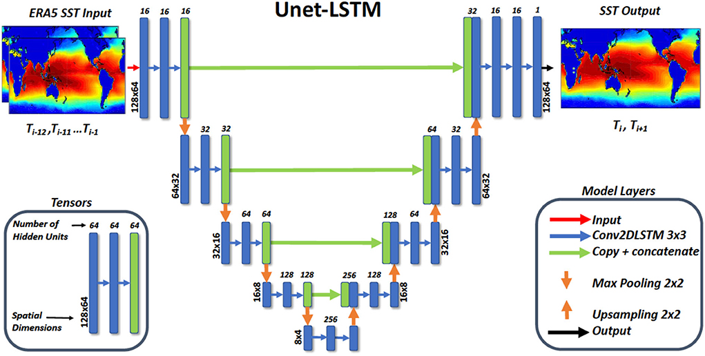
Figure 2. A summary of the architecture of the convolutional neural network (CNN) model, referred to as the Unet-LSTM, that we have trained to forecast 2-D SST fields. The model shown was implemented in Python using the TensorFlow and Keras 2.4 API.

We used 760 of the available time steps from January 1950 to April 2013 for training and the remaining 97 time steps for validation and testing. We have attempted to best balance the need to train the model while testing the model performance to ensure that it is not overfitting and can predict unseen data. Although the validation period is short, it contains several El Nino and La Nina events, which provide a certain degree of freedom to validate the model performance. The Unet-LSTM model uses the prior 12 months of SST data in order to predict the following 2 months of SST data. Note that selecting a longer prediction time period results in errors accumulating over a longer prediction window. We used the tanh activation function, set the kernel, bias and recurrent L2 regularization value at 10^-8, and run the model training for 200 epochs saving only the model with the minimum mean square error (MSE) value, then output the final model and report the resulting MSE values. The MSE value is defined as

$\begin{array}{ll}MSE=\frac{1}{n}{\displaystyle \sum _{i=1}^n}{(y-ŷ)}^2& (1)\end{array}$

where y is the target ECMWF ERA5 SST value, ŷ is the model estimated SST value, and n is the total number of SST values in the training data set. MSE is a standard loss function for regression problems. Mean square log error (MSLE) was also considered but did not lead to significantly improved fit so MSE was preferred. Mean absolute error as a loss function results in a poorer model fit. Land areas were included in the loss function as leaving land areas unconstrained did not lead to an improved fit over the oceans. When we included the land areas, the improvement was small, mostly due to an improvement in the model fit to SSTs at the continental margins.

We found that 200 epochs ensured that the MSE value always reached a minimum without overfitting. Figure 3 shows the MSE error calculated from a comparison of the model predictions with all the training (train) and all the validation (test) data sets converging over a 200 epoch training period. This graph clearly shows that the model is not overfitting and that we can have high confidence in the model as the MSE error for the whole test data is nearly identical to that of the training data. Using the saved model, we then make model predictions (inference) using an autoregressive approach for up to 24 months.

FIGURE 3

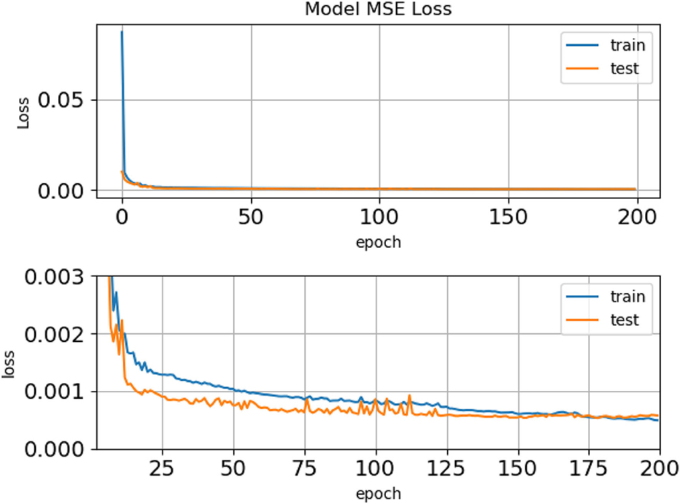
Figure 3. The mean square error (MSE) error calculated from a comparison of the model predictions with the training (train) and the validation (test) data sets over a 200 epoch training period. We see a rapid convergence of the model on the minimum MSE value. The upper panel shows the MSE values over the full 200 epochs. In order to show greater detail of the model fitting process, the lower panel shows the same MSE values at higher resolution and focused on the tail of the model training. Note the different y-axis scales between the two panels.

We applied a standard formula for normalization as is commonly used in deep learning. The minimum (x_min) and maximum SST (x_max) over all the data were calculated and the following formula was applied

$\begin{array}{ll}{z}_i=(x_i-x_{min})/(x_{max}-x_{min})& (2)\end{array}$

where x_i is the raw ECMWF ERA5 SST value and z_i is the normalized ECMWF ERA5 SST value, Normalization primarily aids in numerical stability, thus making a solution possible, and speeding up the rate of convergence to a solution.

In order to efficiently load the model training data using a data-parallel approach, we distribute the model data required by each GPU onto the CPU memory of the corresponding node, as we have done in prior studies (Taylor et al., 2021). The data required on each GPU is read once from a single NetCDF file containing the preprocessed data as described above. This approach facilitates the rapid loading of each batch of data to GPU memory and makes possible the highly scalable data-parallel training by preventing a filesystem IO bottleneck from occurring during training. This is particularly important when training the forecast Unet-LSTM model as we construct a batch using a rolling window from the 12 past time steps and the future 2 time steps, so each sample in a batch consists of a total of 14 time steps. In order to further reduce memory usage for the Unet-LSTM model, we define a data loader so we load from memory only the data that each batch requires at each time step. We divide the training and test data sets equally by time onto each GPU. It is essential that each GPU has exactly the same number of time steps to avoid problems with load balancing and the timely communication of model parameters at the end of each epoch.

3. Results

Having trained the Unet-LSTM model, we can then make forecasts (inferences) of the temporal evolution of the 2-D SST fields. The model inference step takes the preceding 12 months of SST data and makes predictions of the following 2 months. By using an autoregressive approach, where we feed model predictions back in as input to the model, we can make an unlimited number of predictions. For the results reported here, we limit the predictions to a 24-month window. Model predictions span the data used both for model training and validation, noting that the MSE between all the training and all the test data are nearly identical. As the MSE values are nearly identical, looking at results drawn from either the training and or validation periods primarily reflects the response of the model to a particular set of input data. This is the first presentation of the Unet-LSTM model applied to the prediction of global scale SST fields. Future work with longer training and validation periods will provide a more thorough analysis of the model approach.

In this section, we first present results showing the predictions of the global scale SST fields. We also use the global scale SST fields to extract the SST values that correspond with well-known climate indices. As we are making predictions of the global scale fields, we can extract any index of interest from our model predictions without the need to develop and train a new model.

3.1. Global scale 2-D SST predictions

We first show an example set of SST model hindcasts at t=1, 6, 12, and 18 months initiated in the December 2015 El Niño. We are using only the test data set to perform the SST model hindcasts. Figure 4 presents the model predicted SST field at t=1 (January 2016), the corresponding target ECMWF ERA5 SST field, the difference between the model predicted and ERA5 SST, and the model predicted SST anomaly which is the difference between the model predicted SST values and an ERA5 climatology computed over the 30 year period 1981–2010. The model predicted SST values accurately capture the main features of the target ERA5 SST values with the majority of differences in SST values falling within the range ±1°C. There does appear to be evidence that the model is systematically slightly warmer above 20°N and slightly cooler in the eastern pacific below 20°S in Figure 4. The model captures the SST warming in the eastern equatorial Pacific during the 2015–2016 El Niño, though with a small cool bias, or underestimation of the warming. Interestingly, the model is also able to capture the warming SST off the northwest Australian coast. Model predictions of warm SST anomalies in the eastern Mediterranean Sea and northwest Atlantic coast appear also being supported by observations (Figure 4).

FIGURE 4

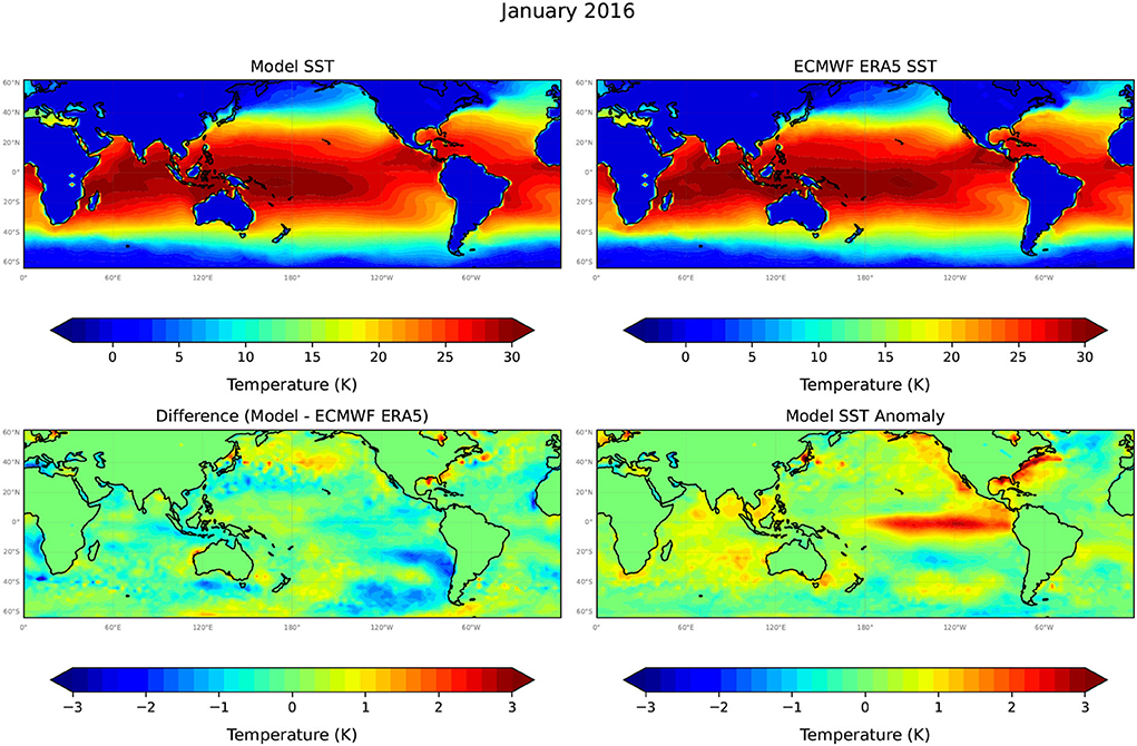
Figure 4. The model predicted SST at +1 month (January 16), from a model forecast initiated in December 2015, the corresponding target ERA5 SST data set, the difference between the model predictions and the target, and the model predicted SST anomaly. Note the different, much higher resolution temperature scale used to plot model differences and SST anomalies.

Figures 5–7 compare Unet-LSTM model predictions at t = 6, 12, and 18 months into the future, respectively. We can see that the model captures the temporal evolution of SST field well over the full 18-month prediction period. The differences between model predicted SST values grow slowly over the 18-month prediction period with the majority of differences in SST values, as shown in Figure 7, falling within the range ±2°C with a small overall bias toward cooler temperatures. The root mean square error (RMSE) value increases steadily over the 18-month prediction period from 0.48°C in January 2016 to 0.63°C in June 2017. At 12 months lead (Figure 6), the Unet-LSTM model predicts the near maximum cooling in the equatorial eastern Pacific as El Niño ends and La Nina conditions develop. At 18 months (Figure 7), the ocean temperatures are predicted to have warmed slightly again, as is seen in the ERA SST data. Thus, there appears to be good skill predicting the cooling at the 12-month lead and warming of SSTs at the 18-month lead time. The model predicted SSTs at mid-to high-latitudes in the southern hemisphere at 18-month lead are biased to cooler temperatures than are seen in the ERA5 data (Figure 7). Nevertheless, the Unet-LSTM model captures the underlying seasonal, and to some extent interannual, variations of the global SST quite accurately.

FIGURE 5

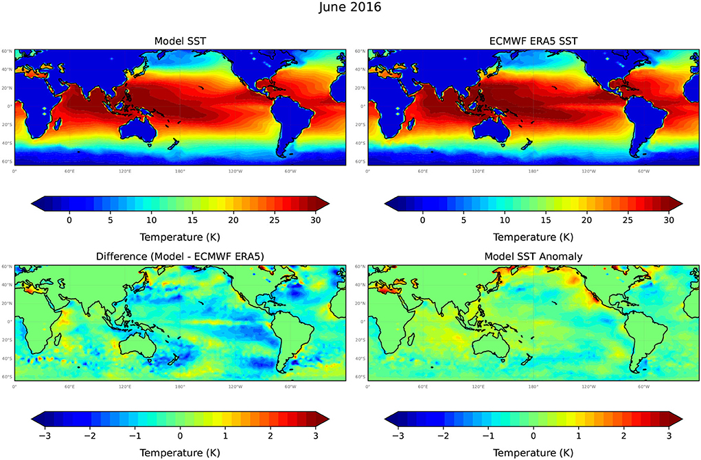
Figure 5. The model predicted SST at +6 months (June 2016), from a model forecast initiated in December 2015, the corresponding target ERA5 SST data set, the difference between the model predictions and the target, and the model predicted SST anomaly. Note the different, much higher resolution temperature scale used to plot model differences and SST anomalies.

FIGURE 6

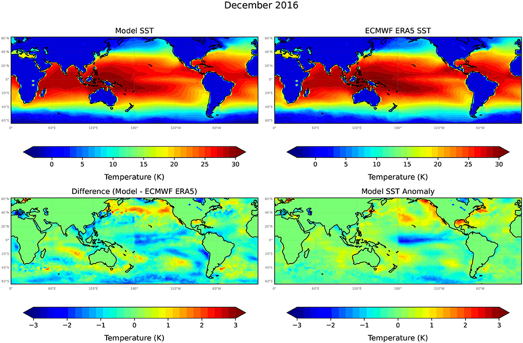
Figure 6. The model predicted SST at +12 months (December 2016), from a model forecast initiated in December 2015, the corresponding target ERA5 SST data set, the difference between the model predictions and the target, and the model predicted SST anomaly. Note the different, much higher resolution temperature scale used to plot model differences and SST anomalies.

FIGURE 7

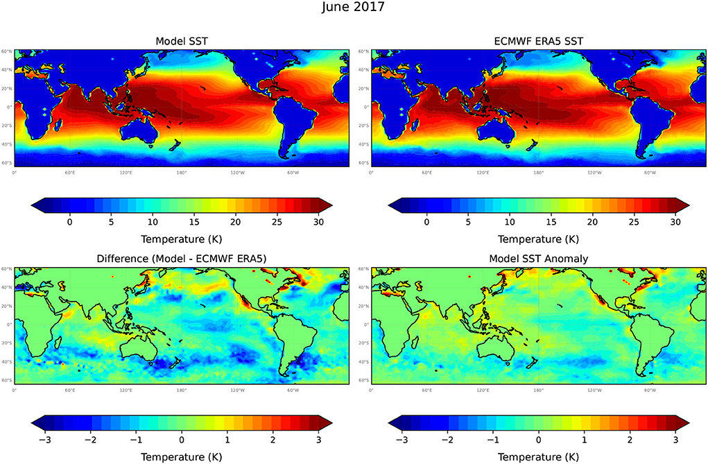
Figure 7. Model predicted SST at +18 months (June 2017), from a model forecast initiated in December 2015, the corresponding target ERA5 SST data set, the difference between the model predictions and the target, and the model predicted SST anomaly. Note the different, much higher resolution temperature scale used to plot model differences and SST anomalies.

Figure 8 presents histograms of the Unet-LSTM model predicting SST values in comparison with the ERA5 SST values for June 2017, corresponding to the results presented in Figure 7, at the end of the 18 month prediction period. Figure 8 clearly demonstrates that the model is able to accurately maintain the correct distribution of SST values with no smearing of the distribution even at the end of the 18 month prediction window. This can be attributed to the use of the Conv2DLSTM layers in the Unet-LSTM model which correctly captures both the spatial and temporal evolution of the 2D SST field. The second panel in Figure 8 shows a histogram of the differences between the model and the ERA5 SST values in comparison with errors produced by assuming persistence from December 2015. The histogram of the model differences is centered close to 0°C with the majority of errors falling within the range ±2°C, as previously shown in Figure 7.

FIGURE 8

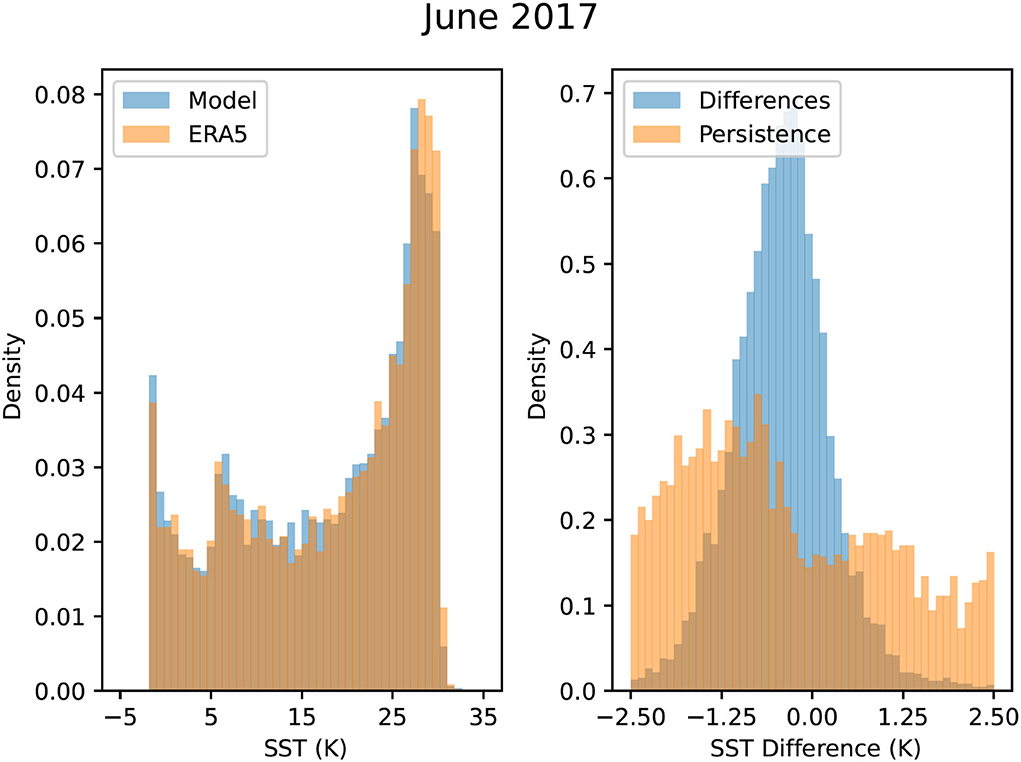
Figure 8. Histograms of the model predicted SST values in comparison with the ERA5 SST values for June 2017 at the end of the 18-month prediction period. The second panel shows a histogram of the differences between the model and the ERA5 SST values in comparison with errors produced by assuming persistence.

Figure 9 shows the estimates of the Pearson correlation index for our predicted SST against the ERA5 SST data based on the 10 24-month predictions starting in July 2006 from months t+1 to t+6. Figure 10 shows a corresponding plot to Figure 9 except for the months t+7 to t+12. In order to be able to compute the Pearson correlation index over 10 years part of the data for the correlation analysis is from the training period. As illustrated in Figure 3, the MSE errors for the training and test periods are nearly identical indicating that data from the training period will not overly influence the results. The case studies in the model validation period of the study also tend to support the correlation analysis. Future studies will further address this issue.

FIGURE 9

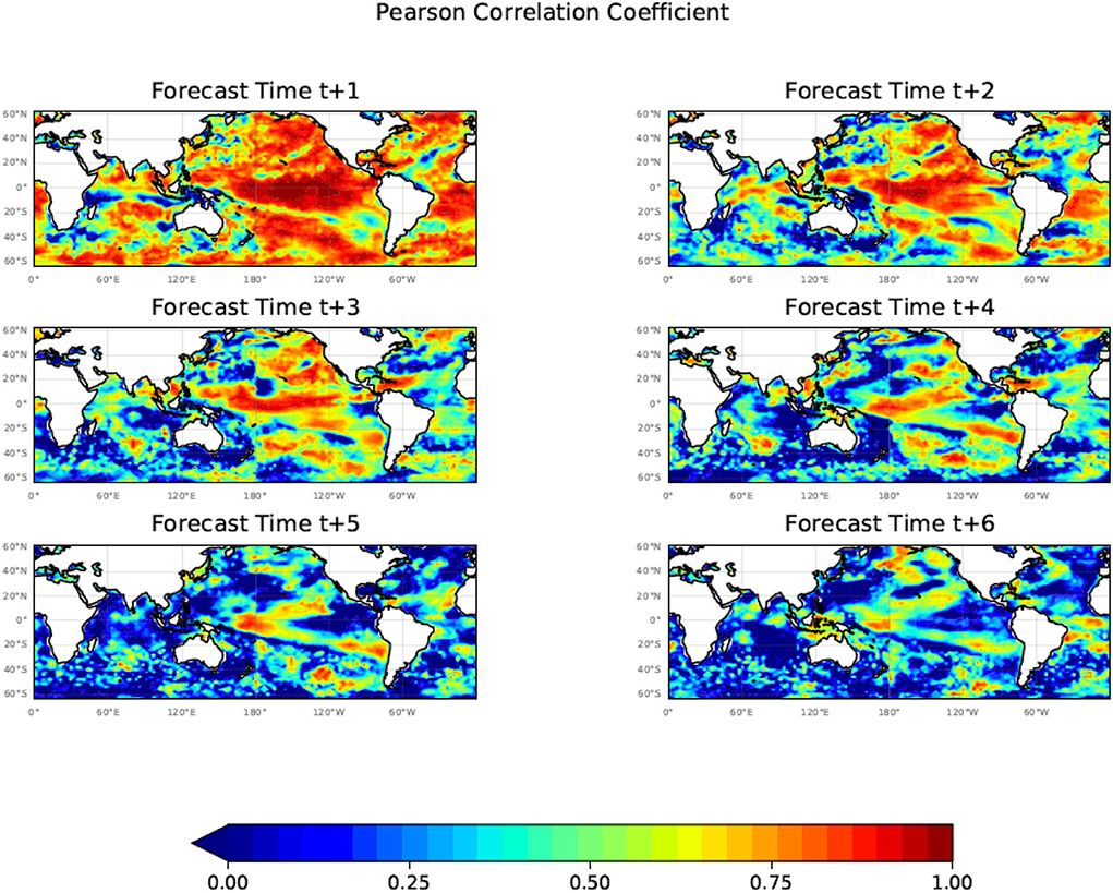
Figure 9. The Pearson correlation coefficient (R) calculated using the 10 24-month forecasts commencing each July from July 2006 until July 2015 for months t+1 to t+6 showing large regions of significant correlation between the model predicted and ERA5 SST values out to t+6. In order to use a 10-year period, part of the data for the correlation analysis is from the training period, however, the case studies in the model validation period of the study tend to support the correlation analysis.

FIGURE 10

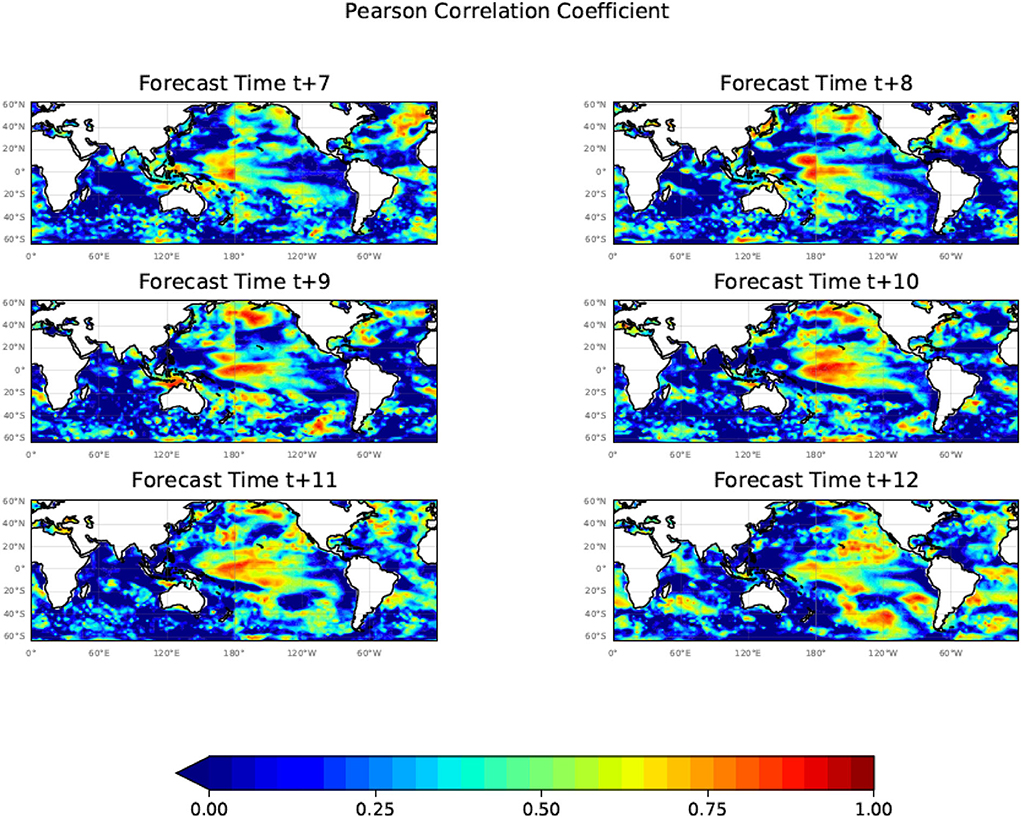
Figure 10. The Pearson correlation coefficient (R) calculated using the 10 24-month forecasts commencing each July from July 2006 to July 2015 for months t+7 to t+12 showing the presence of a significant correlation between the model predicted and ERA5 SST values out to t+12. In order to use a 10-year period, part of the data for the correlation analysis is from the training period, however, the case studies in the model validation period of the study tend to support the correlation analysis.

Figures 9, 10 illustrate that the Unet-LSTM model is able to maintain a good correlation with the target ERA5 SST anomalies for predictions out to t+12 months. Not shown are plots of the Pearson correlation index for t+13 to t+24 which continue to show regions of significant correlation. In general, long-lead high prediction skills are mostly located in the tropical, northeast, and south Pacific. There are also high prediction skills for the high latitude North Atlantic. There are good skills for the Indian Ocean Dipole regions up to 3-month lead, and the skills decay rapidly, likely due to a winter prediction barrier of the IOD (e.g., Luo et al., 2007). The high predictability regions from the Unet-LSTM model are consistent with a statistical predictability analysis of monthly SST anomalies in the global ocean (Li and Ding, 2013), with high predictability in the tropical eastern Pacific, tropical western Indian Ocean, and tropical Atlantic, and mid-latitude Pacific (their Figure 2).

3.2. Long-lead predictions of the El Niño 3.4 and El Niño 4 indices

Most dynamic models' correlation prediction skills drop to around 0.5 at a 12-month lead for Nino3.4, as presented recently (Ham et al., 2019). The CNN model developed by Ham et al. (2019) can achieve a longer lead prediction for Nino3.4, however, that is only for a single climate index, whereas in our model we make predictions of the 2-d monthly SST field and Nino3.4 is just one region embedded in the global field. So far, there has not been much study on the prediction skills of global SST.

Using the Unet-LSTM predicted SST values, we can calculate the Niño 3.4 index computed over the region 5°S-5°N, 170°W-120°W. We compared the model predictions with the Niño 3.4 index derived from the ERA5 SST data. The ERA5 Niño 3.4 index is defined as the difference between the monthly mean ERA5 SST values and an ERA5 climatology computed over the 30 year period 1981–2010.

We evaluated the Unet-LSTM model predictions of the Nino 3.4 index during 2015–2020 at various lead times and compared with the consolidated predictions archived at the National Oceanic and Atmospheric Administration (NOAA) Climate Prediction Center (CPC) website (https://iri.columbia.edu/~forecast/ensofcst/Data/) (Figure 11). The CPC consolidated predictions are 3-month averages for up to a 9-month lead. Note that the consolidated prediction data are for 1–9 months leads and are only available after 2015. Rojo Hernández et al. (2020) provided a comprehensive analysis of the forecasting skills of various models archived on the CPC website.

FIGURE 11

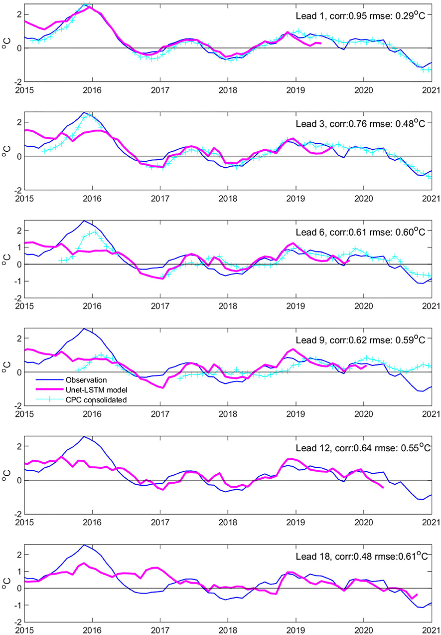
Figure 11. Comparison between the Unet-LSTM model predictions of the Nino3.4 index during 2015-2020 and the consolidated predictions of the National Oceanic and Atmospheric Administration (NOAA) archived at the Climate Prediction Center (CPC) website (https://iri.columbia.edu/~forecast/ensofcst/Data/archive/), with lead times of 1, 3, 6, 9, 12, and 18 months. The correlation and RMSE numbers are denoted for each lead time. The NOAA consolidated predictions are 3-month averages for up to a 9-month lead. In 2016, there are no NOAA consolidated predictions during the first 6 months. The ERA5 monthly Nino3.4 SST anomalies are plotted as references.

Compared with the CPC consolidated prediction, the Unet-LSTM model tends to underestimate the 2015–2016 El Nino SST warming peak at 3–6 month lead; however, the Unet-LSTM model tends to behave better at long leads and can predict a moderate warming in the Nino3.4 region during the 2015–2016 event at up to 18-month lead (Figure 11). Note that the Unet-LSTM model overestimates the amplitude of the weak 2014-15 El Nino event. The Unet-LSTM model predicts the 2018–2019 El Nino event rather accurately at all lead times, up to 18 months, having better skills than the CPC consolidated prediction at long lead times. The Unet-LSTM model may also have long-lead prediction skills for the 2020–2021 La Nina event. In general, the RMSE and correlation skills of the Unet-LSTM model only decrease slightly between 6 and 18 month lead times.

As the 2009-10 El Niño is generally regarded as a central Pacific El Niño (Timmermann et al., 2018), we also assess the prediction of Niño 4 SST variability, an index for the central Pacific warming. The Niño 4 index is computed over the region 5°S-5°N and 160°E-150°W. In Figure 12, the upper panel shows the ERA5 Niño 4 index over the 24 months covering the 2009–2010 warm event. The lower panel in Figure 12 presents the spatial pattern of the model predicted SST anomalies in November 2009 taken from the corresponding Niño 4 index predictions in the panel above. It is shown that the model can predict the Niño 4 index variability well, though, with an early peak in the predicted SST anomalies in October 2009 (Figure 12), the warming pattern is similar to a central El Niño event (Figure 12). Note that data from 2009–2010 are from the end of the model training period, as there is no good example for a central Pacific El Nino during the model validation period.

FIGURE 12

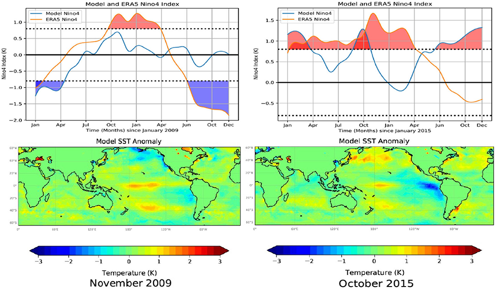
Figure 12. Model predictions of the El Niño 4 index for the 2009-10 and 2015-16 warm periods are presented in the upper panels. In each graph, we compare the model results with the El Niño 4 index, defined as the monthly average SST computed over the region 5°N-5°S and 160°E-150°W, calculated from the monthly mean ERA5 SST data. The dotted lines define warm (> 0.8°C) and cold (< −0.8°C) periods. Model predictions and ERA5 estimates of the El Niño 4 index > 0.8°C have been shaded red, and values < −0.8°C have been shaded blue, for emphasis. The lower panels present the spatial pattern of the model predicted SST anomalies in November 2009 and October 2015 taken from the corresponding 24-month predictions shown in the upper panels. The 2009-10 El Nino is from the model training period, as there is no good example for a central Pacific El Nino during the model validation period.

Figure 13 shows model predictions of the El Niño 3.4 index for a 24-month prediction starting in July 2014 (rather than in January) and ending in June 2016 which spans the entire 2 year warm period. Figure 13 illustrates that the model is able to capture this unusual event with two consecutive El Niños with model predictions tracking the ERA5 El Niño 3.4 index within 1°C, throughout the full 2-year period, though it still does not match the full intensity of the 2015–2016 El Niño. As demonstrated in the correlation maps, we note that most of the ENSO events can be well captured by the Unet-LSTM model.

FIGURE 13

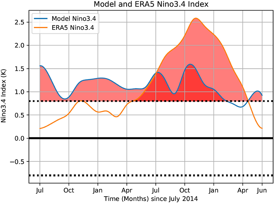
Figure 13. Model predictions of the El Niño 3.4 index for a 24-month prediction starting in July 2014 and ending in June 2016. We compare the model results with the El Niño 3.4 index, defined as the monthly average SST computed over the region 5°N-5°S and 120°W-170°W, calculated from the monthly mean ERA5 SST data. The dotted lines define warm (> 0.8°C) and cold (< −0.8°C) periods. Model predictions and ERA5 estimates of the El Niño 3.4 index > 0.8°C have been shaded red, and values < −0.8°C have been shaded blue, for emphasis.

3.3. Long-lead predictions of the “Blob” index

We have computed the Blob index using the ERA5 SST data for the period January 1950-May 2021. The Blob index is defined as the difference between the monthly average SST climatology (1981–2010) and the monthly average SST computed over the region 34°N-47°N, 147°W-128°W (Amaya et al., 2020). Figure 14 presents the blob index over this time period, along with a two-sided 95% confidence interval and a one-sided 90% confidence interval. In the lower panel of Figure 14, we focus on the period January 2014-May 2021. During this time period, we see multiple exceptional ocean warming events in the Blob region where ocean temperatures exceed the 95% confidence interval by up to 1°C. It is also worth noting during the January 2014-May 2021 period the Blob index only dropped below 0°C during the boreal winter of 2016–2017.

FIGURE 14

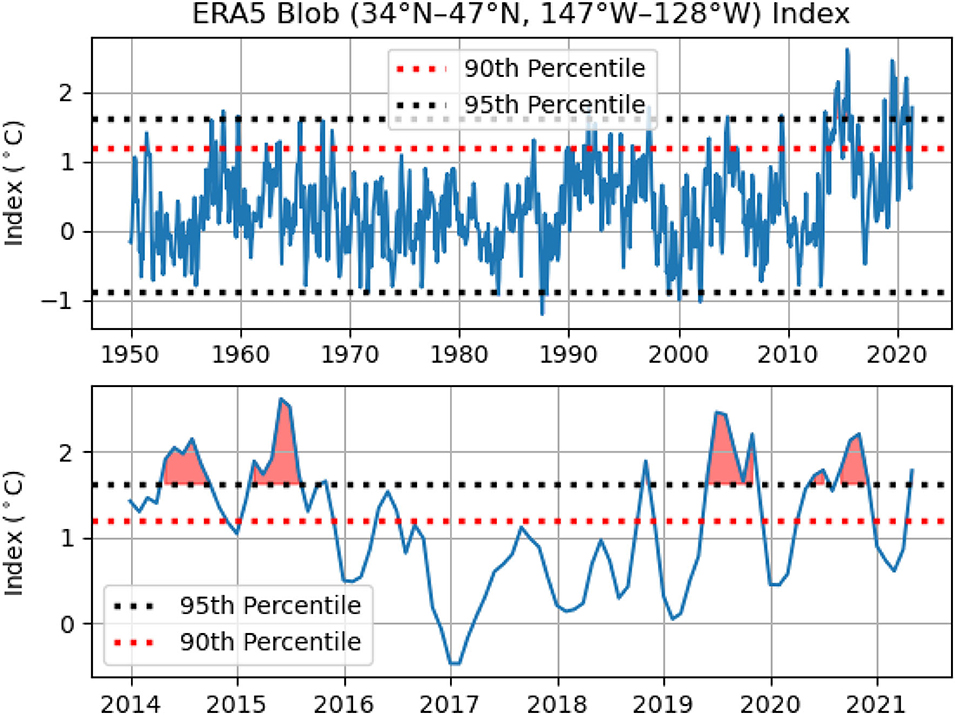
Figure 14. The Blob index defined as the difference between the monthly average SST climatology (1981–2010) and the monthly average SST computed over the region 34°N-47°N and 147°W-128°W. We compute the Blob index from the monthly mean ERA5 SST data for the period January 1950-May 2021. We include the two-sided 95% confidence interval and the one-sided 90th percentile. The lower panel is the same Blob index with a focus on the period January 2014-May 2021 with the significant ocean warming events in 2014, 2015, 2019, and 2020 highlighted.

In order to demonstrate the ability of the Unet-LSTM model to predict the Blob index, Figure 15 presents multiple 24 month predictions of the Blob index focusing on the period 2014–2021. The Unet-LSTM model Blob index is computed from the corresponding model predicted SST values, e.g., as presented in Figures 4–7 and monthly average SST climatology (1981–2010). We include 24-month predictions that capture the warm events in 2014 and 2015, the cooling during the winter of 2016–2017, and the two warm events in 2019 and 2020. Figure 15 illustrates the ability of the model to accurately predict the evolution of the Blob index during both warming and cooling events over the full 24-month prediction period.

FIGURE 15

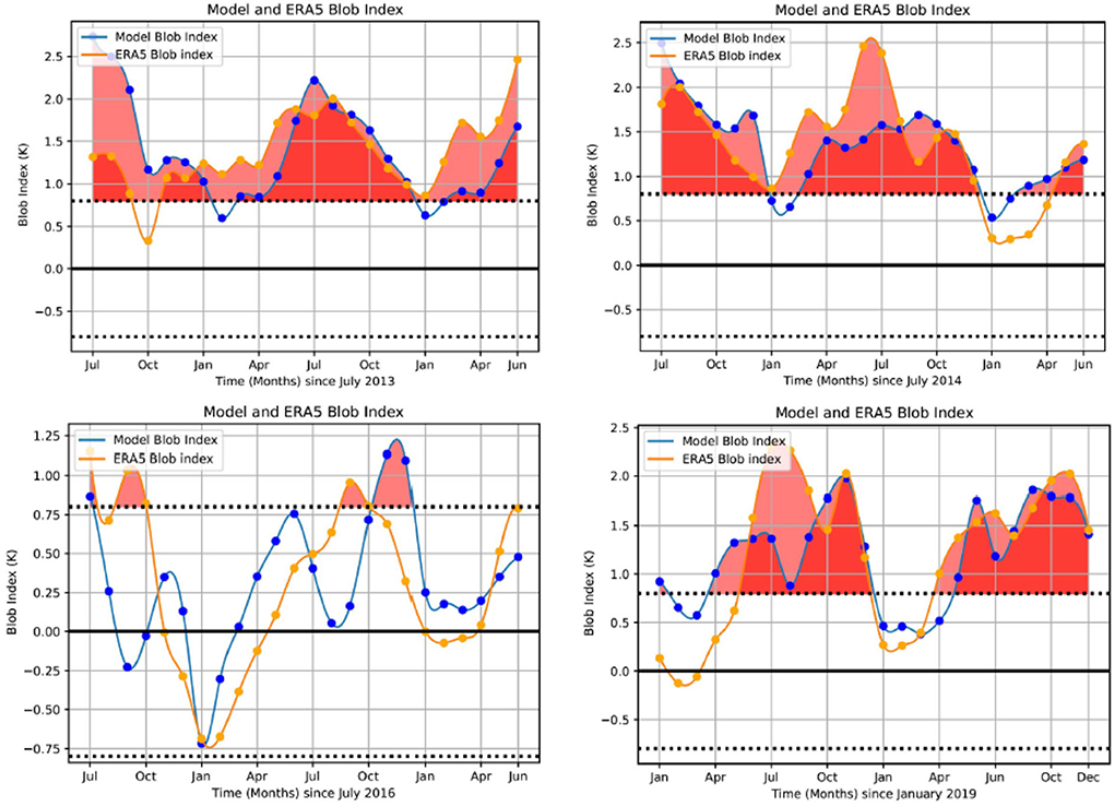
Figure 15. Model predictions of the Blob index over a 24 month period commencing in July 2013, 2014, 2015, and January 2019 compared with the Blob index, defined as the monthly average SST computed over the region 34°N-47°N and 147°W-128°W, calculated from the monthly mean ERA5 SST data. We include the two-sided 95% confidence interval. We focus on the period January 2014-May 2021 with the significant ocean warming events in 2014 and 2015 captured in the top two panels. The winter cooling in 2016–2017 and the warming events in 2019 and 2020 are presented in the lower panels.

4. Summary and discussion

In this study, we use monthly reanalysis of global surface temperature (SST and 2-m air temperature) data to train a Unet-LSTM data-driven model and demonstrate its ability to predict SST variability at various lead times. We used a 12-month window to train the Unet-LSTM model, with the seasonal cycles retained in the training data, which effectively captured the seasonal SST variation in the global ocean. For the SST anomaly prediction, there are high long-lead skills in the equatorial Pacific and northeast Pacific. In the following, we discuss a few aspects of the model predictions and outline our plans for future work.

4.1. Comparison with other ML ENSO prediction architectures

Ham et al. (2019) developed a CNN deep learning model, trained with coupled climate model outputs, to achieve 18-month-lead prediction skills for Nino3.4. Their model was initialized with both monthly SST and upper ocean heat content anomalies, claiming that the upper ocean heat content memory actually helped the model to achieve the long-lead model skills. Most of the recent development in deep learning ENSO forecasting models are based on this framework (Ham et al., 2021 among others). The Unet-LSTM based CNN model trained and initialized with global surface temperature fields can achieve similar prediction skills, not only for Nino3.4 but also in the northeast Pacific, which is demonstrated in the prediction assessment of the recent Blob marine heatwave events.

We have used a 12-month window to train the Unet-LSTM model, while most other CNN models used 3-month temporal window. The model achieves long-lead prediction mostly in the Pacific, which suggests that the precursors of the long-lead prediction likely reside in the Pacific.

By using a 12-month time window to train the Unet-LSTM model, we can use the full temperature field, instead of only using the anomaly field. In this way, both the annual cycle of temperature variations and the interannual anomalies are considered simultaneously. This may have two benefits: one is to be able to train the model to assimilate the dynamics of the seasonally phase-locked variability; the other is that the model can carry the memory over the past years, so that it is not necessary to remove the steady warming trend at the surface ocean from the reanalysis (observation) data prior to the model training.

Note that there is an attempt to capture the seasonal cycle by introducing additional labels in a CNN model (Ham et al., 2021); however, it may only be achievable for a single index prediction. However, we do need to assess the stability of the model prediction starting from different months, especially when there are known prediction barriers for various climate indices (e.g., Timmermann et al., 2018). While the Unet-LSTM model is able to predict most ENSO events well, it is noted that the model prediction starting in January fails to predict the 2015–2016 peak during the rare occurrence of two consecutive El Ninos, likely due to a lack of similar cases in the training data based on existing observations. ENSO diversity may still pose a challenge for data-driven ML models. Nevertheless, the current version of Unet-LSTM shows great promise in leading the way to more sophisticated 2-dimensional SST predictions for the global ocean.

4.2. Future work

The success of the Unet-LSTM model at capturing key features of the global scale temperature field clearly demonstrates that data-driven approaches to modeling the spatio-temporal evolution of complex physical systems such as SSTs are a promising avenue for further research. As a next step, we plan to retrain our model using the twentieth-century reanalysis products with a more extended validation period in future studies. We also plan to increase the model spatial resolution to the full resolution of the ERA5 data set, currently 0.25°, which will allow us to investigate the impact of model resolution on SST predictions and to study the variations in SST at the regional scale in more detail. Incorporating upper ocean variability as model input is also a priority. It appears that some upper ocean memory may reside in the surface temperature records. Surface SST and land surface temperatures drive global surface wind anomalies and then subsequently drive the planetary ocean waves to store the upper ocean heat content anomalies. This is a problem for further exploration. We will also investigate better quantifying the uncertainty associated with model forecasts using an ensemble forecasting approach and the prediction of other key ocean indices, such as the Indian Ocean Dipole (IOD), using both the existing model and at higher model resolutions.

Given the results presented here and the successful application of the Unet-LSTM model in previous studies (Taylor et al., 2021), we have increased confidence that the Unet-LSTM model can be applied to the general problem of the spatial and temporal evolution of other 2D geophysical fields. As of TensorFlow 2.6, a ConvLSTM3D layer is now available. By replacing the ConvLSTM2D layer with the ConvLSTM3D layer, the Unet-LSTM can be used to predict the spatio-temporal evolution of 3D fields. The ability to model 3D fields will allow us to investigate improving SST predictions by incorporating additional input variables, such as surface wind fields, into the Unet-LSTM model. The primary barrier to working with large 3D fields is the availability of GPU memory which on current devices is limited to 16-32GB. Next, generation GPU devices will have significantly larger memory, which combined with model parallelism, will allow much larger more complex models to be developed.

Training the Unet-LSTM model only with the reanalyzed temperature field (which incorporates existing observations) over the seven decades appears to have constrained the model to capture the ENSO dynamics and its teleconnection in the Indian Ocean and mid-latitude oceans (e.g., the Blob region). On the other hand, the CNN ML models are trained using coupled atmosphere-ocean models, which have inherent biases in the coupled models, as well as unrealistic ENSO simulations in some of the coupled models, such as the ENSO frequencies. Transfer learning, which has been proposed in some studies (Ham et al., 2019), may not be enough to correct these model biases (Timmermann et al., 2018). A knowledge-based strategy is needed to combine the coupled model results with observations to provide a well-sampled dataset, for the ML models to capture the diverse SST variability in the global and regional oceans, in order to better predict rare climate events.

A new and rapidly evolving area of research is physics-informed ML (Karniadakis et al., 2021) that combines ML with physical constraints, derived for example, from ordinary differential equations (ODEs) and partial differential equations (PDEs) that describe the system under study. The implementation of physics-informed ML is mesh-less which allows model regression to take place using an available set of imperfect observations that define the initial and boundary conditions without the need to interpolate the data to an appropriate grid. Physics-informed ML could yield new, more flexible, potentially transformative, approaches to ocean modeling; however much work needs to be done to realize this goal.

Data availability statement

The datasets presented in this study can be found in online repositories. The names of the repository/repositories and accession number(s) can be found below: dap.csiro.au.

Author contributions

Both authors listed have made a substantial, direct, and intellectual contribution to the work and approved it for publication.

Funding

This research project was undertaken with the assistance of the resources and services from the National Computational Infrastructure (NCI), which is supported by the Australian Government. MF was also supported by the Centre for Southern Hemisphere Oceans Research (CSHOR), which was a joint initiative between the Qingdao National Laboratory for Marine Science and Technology (QNLM), CSIRO, University of New South Wales and University of Tasmania.

Conflict of interest

The authors declare that the research was conducted in the absence of any commercial or financial relationships that could be construed as a potential conflict of interest.

Publisher's note

All claims expressed in this article are solely those of the authors and do not necessarily represent those of their affiliated organizations, or those of the publisher, the editors and the reviewers. Any product that may be evaluated in this article, or claim that may be made by its manufacturer, is not guaranteed or endorsed by the publisher.

References

Abadi, M., Agarwal, A., Barham, P., Brevdo, E., Chen, Z., Citro, Z., et al. (2015). TensorFlow: Large-scale machine learning on heterogeneous systems. arXiv [Preprint]. arXiv: 1603.04467. Available online at: https://arxiv.org/pdf/1603.04467.pdf

Google Scholar

Amaya, D. J., Miller, A. J., Xie, S. P., and Kosaka, Y. (2020). Physical drivers of the summer 2019 North Pacific marine heatwave. Nat. Commun. 11, 1903. doi: 10.1038/s41467-020-15820-w

PubMed Abstract | CrossRef Full Text | Google Scholar

Badrinarayanan, V., Kendall, A., and Cipolla, R. (2017). SegNet: a deep convolutional encoder-decoder architecture for image segmentation. IEEE Trans. Pattern Anal. Mach. Intell. 39, 2481–2495. doi: 10.1109/TPAMI.2016.2644615

PubMed Abstract | CrossRef Full Text | Google Scholar

Bond, N. A., Cronin, M. F., Freeland, H., and Mantua, N. (2015). Causes and impacts of the 2014 warm anomaly in the NE Pacific. Geophys. Res. Lett. 42, 3414–3420. doi: 10.1002/2015GL063306

CrossRef Full Text | Google Scholar

Chollet, F. (2015). Keras.

Google Scholar

Di Lorenzo, E., and Mantua, N. (2016). Multi-year persistence of the 2014/15 North Pacific marine heatwave. Nat. Clim. Chang. 6, 1042–1047. doi: 10.1038/nclimate3082

CrossRef Full Text | Google Scholar

Doi, T., Behera, S. K., and Yamagata, T. (2013). Predictability of the Ningaloo Niño/Niña. Sci. Rep. 3, 2892. doi: 10.1038/srep02892

PubMed Abstract | CrossRef Full Text | Google Scholar

Feng, M., Hendon, H. H., Xie, S. P., Marshall, A. G., Schiller, A., Kosaka, Y., et al. (2015). Decadal increase in Ningaloo Niño since the late 1990s. Geophys. Res. Lett. 42, 104–112. doi: 10.1002/2014GL062509

CrossRef Full Text | Google Scholar

Feng, M., McPhaden, M. J., Xie, S. P., and Hafner, J. (2013). La Niña forces unprecedented Leeuwin Current warming in 2011. Sci. Rep. 3, 1277. doi: 10.1038/srep01277

PubMed Abstract | CrossRef Full Text | Google Scholar

Gupta, A., Thomsen, M., Benthuysen, J. A., Hobday, A. J., Oliver, E., Alexander, L. V., et al. (2020). Drivers and impacts of the most extreme marine heatwaves events. Sci. Rep. 10, 19359. doi: 10.1038/s41598-020-75445-3

PubMed Abstract | CrossRef Full Text | Google Scholar

Ham, Y., Kim, J., and Luo, J. (2019). Deep learning for multi-year ENSO forecasts. Nature 573, 7775. doi: 10.1038/s41586-019-1559-7

PubMed Abstract | CrossRef Full Text | Google Scholar

Ham, Y. G., Kim, J. H., Kim, E. S., and On, K. W. (2021). Unified deep learning model for El Niño/Southern Oscillation forecasts by incorporating seasonality in climate data. Sci. Bull. 66, 1358–1366. doi: 10.1016/j.scib.2021.03.009

CrossRef Full Text | Google Scholar

Hersbach, H., Bell, B., Berrisford, P., Hirahara, S., Horányi, A., Mu noz-Sabater, J., et al. (2020). The ERA5 global reanalysis. Q. J. R. Meteorol. Soc. 146, 1358–1366. doi: 10.1002/qj.3803

CrossRef Full Text | Google Scholar

Hochreiter, S., and Schmidhuber, J. (1997). Long short-term memory. Neural Comput. 9, 1735–1780. doi: 10.1162/neco.1997.9.8.1735

PubMed Abstract | CrossRef Full Text | Google Scholar

Holbrook, N. J., Scannell, H. A., Sen Gupta, A., Benthuysen, J. A., Feng, M., Oliver, E. C., et al. (2019). A global assessment of marine heatwaves and their drivers. Nat. Commun. 10, 2624. doi: 10.1038/s41467-019-10206-z

PubMed Abstract | CrossRef Full Text | Google Scholar

Karniadakis, G. E., Kevrekidis, I. G., Lu, L., Perdikaris, P., Wang, S., and Yang, L. (2021). Physics-informed machine learning. Nat. Rev. Phys. 3, 422–440. doi: 10.1038/s42254-021-00314-5

CrossRef Full Text | Google Scholar

Kataoka, T., Tozuka, T., Behera, S., and Yamagata, T. (2014). On the Niño/Niña. Clim. Dyn. 43, 1463–1482. doi: 10.1007/s00382-013-1961-z

CrossRef Full Text | Google Scholar

Kingma, D. P., and Ba, J. L. (2014). “Adam: a method for stochastic optimization,” in 3rd International Conference on Learning Representations, ICLR 2015-Conference Track Proceedings (San Diego) (ArxIV). doi: 10.48550/arXiv.1412.6980

CrossRef Full Text | Google Scholar

Larraondo, P. R., Renzullo, L. J., Inza, I., and Lozano, J. A. (2019). A data-driven approach to precipitation parameterizations using convolutional encoder-decoder neural networks. Technical report.

Google Scholar

Li, J., and Ding, R. (2013). Temporal-spatial distribution of the predictability limit of monthly sea surface temperature in the global oceans. Int. J. Climatol. 33, 1936–1947. doi: 10.1002/joc.3562

CrossRef Full Text | Google Scholar

Luo, J. J., Masson, S., Behera, S., and Yamagata, T. (2007). Experimental forecasts of the Indian Ocean dipole using a coupled OAGCM. J. Clim. 20, 2178–2190. doi: 10.1175/JCLI4132.1

CrossRef Full Text | Google Scholar

McPhaden, M. J., Zebiak, S. E., and Glantz, M. H. (2006). ENSO as an integrating concept in earth science. Science 314, 1740–1745. doi: 10.1126/science.1132588

PubMed Abstract | CrossRef Full Text | Google Scholar

NCI (2020). ERA5 Replicated Datasets.

Google Scholar

Ratnam, J. V., Dijkstra, H. A., and Behera, S. K. (2020). A machine learning based prediction system for the Indian Ocean Dipole. Sci. Rep. 10, 284. doi: 10.1038/s41598-019-57162-8

PubMed Abstract | CrossRef Full Text | Google Scholar

Rojo Hernández, J. D., Mesa, Ó. J., and Lall, U. (2020). Enso dynamics, trends, and prediction using machine learning. Weather For. 35, 2061–2081. doi: 10.1175/WAF-D-20-0031.1

CrossRef Full Text | Google Scholar

Ronneberger, O., Fischer, P., and Brox, T. (2015). “U-net: convolutional networks for biomedical image segmentation,” in Lecture Notes in Computer Science (including subseries Lecture Notes in Artificial Intelligence and Lecture Notes in Bioinformatics), Vol. 9351 (Verlag: Springer), 234–241.

Google Scholar

Saji, N. H., and Yamagata, T. (2003). Possible impacts of Indian Ocean Dipole mode events on global climate. Clim. Res. 25, 151–169. doi: 10.3354/cr025151

CrossRef Full Text | Google Scholar

Schulzweida, U. (2019). CDO User's Guide. Technical Report June.

Google Scholar

Sergeev, A., and Del Balso, M. (2018). Horovod: fast and easy distributed deep learning in TensorFlow. arXiv [Preprint]. arXiv: 1802.05799. doi: 10.48550/arXiv.1802.05799

CrossRef Full Text | Google Scholar

Simmons, A., Hersbach, H., Munoz-Sabater, J., Nicolas, J., Vamborg, F., Berrisford, P., et al. (2021). Low frequency variability and trends in surface air temperature and humidity from ERA5 and other datasets. Technical Report 881, ECMWF, Reading.

Google Scholar

Simonyan, K., and Zisserman, A. (2015). “Very deep convolutional networks for large-scale image recognition,” in 3rd International Conference on Learning Representations, ICLR 2015-Conference Track Proceedings.

Google Scholar

Spillman, C. M., and Smith, G. A. (2021). A new operational seasonal thermal stress prediction tool for coral reefs around Australia. Front. Mar. Sci. 8, 687833. doi: 10.3389/fmars.2021.687833

CrossRef Full Text | Google Scholar

Stockdale, T. N., Anderson, D. L., Balmaseda, M. A., Doblas-Reyes, F., Ferranti, L., Mogensen, K., et al. (2011). ECMWF seasonal forecast system 3 and its prediction of sea surface temperature. Clim. Dyn. 37, 455–471. doi: 10.1007/s00382-010-0947-3

PubMed Abstract | CrossRef Full Text | Google Scholar

Taylor, J. (2021). unet_lstm - A Machine Learning Model for the Spatial and Temporal Evolution of 2D and 3D Fields. v1. CSIRO. doi: 10.25919/3tvm-fw28

CrossRef Full Text | Google Scholar

Taylor, J. A., Larraondo, P., and de Supinski, B. R. (2021). Data-driven global weather predictions at high resolutions. Int. J. High Perform. Comput. Appl. 36, 130–140. doi: 10.21203/rs.3.rs-310930/v1

CrossRef Full Text | Google Scholar

Timmermann, A., An, S. I., Kug, J. S., Jin, F. F., Cai, W., Capotondi, A., et al. (2018). El Ni no-Southern Oscillation complexity. Nature 559, 535–545. doi: 10.1038/s41586-018-0252-6

PubMed Abstract | CrossRef Full Text | Google Scholar

Tozuka, T., Feng, M., Han, W., Kido, S., and Zhang, L. (2021). “The Ningaloo Niño/Niña: mechanisms, relation with other climate modes and impacts,” in Tropical and Extratropical Air-Sea Interactions (Elsevier), 207–219. doi: 10.1016/B978-0-12-818156-0.00006-X

CrossRef Full Text | Google Scholar