 James M. Thornton
 Nicholas Pepin2
 Carolina Adler
95% of researchers rate our articles as excellent or good
Learn more about the work of our research integrity team to safeguard the quality of each article we publish.
Find out more
ORIGINAL RESEARCH article
Front. Clim. , 26 April 2022
Sec. Predictions and Projections
Volume 4 - 2022 | https://doi.org/10.3389/fclim.2022.814181
This article is part of the Research Topic Knowledge Gaps from the IPCC Special Report on the Ocean and Cryosphere in a Changing Climate and Recent Advances, Volume II View all 7 articles
Many mountainous environments and ecosystems around the world are responding rapidly to ongoing climate change. Long-term climatological time-series from such regions are crucial for developing improving understanding of the mechanisms driving such changes and ultimately delivering more reliable future impact projections to environmental managers and other decision makers. Whilst it is already established that high elevation regions tend to be comparatively under-sampled, detailed spatial and other patterns in the coverage of mountain climatological data have not yet been comprehensively assessed on a global basis. To begin to address this deficiency, we analyse the coverage of mountainous records from the Global Historical Climatological Network-Daily (GHCNd) inventory with respect to space, time, and elevation. Three key climate-related variables—air temperature, precipitation, and snow depth—are considered across 292 named mountain ranges. Several additional datasets are also introduced to characterize data coverage relative to topographic, hydrological, and socio-economic factors. Spatial mountain data coverage is found to be highly uneven, with station densities in several “Water Tower Units” that were previously identified as having great hydrological importance to society being especially low. Several mountainous regions whose elevational distribution is severely undersampled by GHCNd stations are identified, and mountain station density is shown to be only weakly related to the human population or economic output of the corresponding downstream catchments. Finally, we demonstrate the capabilities of a script (which is provided in the Supplementary Material) to produce detailed assessments of individual records' temporal coverage and measurement quality information. Overall, our contribution should help international authorities and regional stakeholders identify areas, variables, and other monitoring-related considerations that should be prioritized for infrastructure and capacity investment. Finally, the transparent and reproducible approach taken will enable the analysis to be rapidly repeated for subsequent versions of GHCNd, and could act as a basis for similar analyses using other spatial reporting boundaries and/or environmental monitoring station networks.
Sufficiently lengthy and spatially dense ground-based (or in situ) measurements of climatological and climate-dependent environmental variables contribute to a broad array of applications across the Earth and environmental sciences. Such applications include directly tracking climate and Earth System responses to changes in anthropogenic and natural forcing (for instance via trend analyses of both mean and more extreme conditions; Sun et al., 2021), providing a basis for the generation of gridded (i.e., gap-filled) data products via interpolation (e.g., Harris et al., 2020), and informing the downscaling, bias-correction, and evaluation of climate model reanalyses and future projections (e.g., CH2018, 2018; Zhong et al., 2021). Such observations are also used extensively to force, calibrate, and/or evaluate the models—be they empirical or more process-based—used to generate projections of climate change impacts on various aspects of the cryosphere, hydrosphere, and biosphere (Strachan et al., 2016). Numerical Weather Prediction (NWP) and flood forecasting models likewise routinely assimilate in situ observations to maximize the quality of the short-term forecasts they provide. Lastly, the calibration and evaluation (a.k.a “ground-truthing”) of remote sensing retrieval algorithms also depend heavily on the existence of a sufficient quantity of informative in situ data available (e.g., Dong, 2018).
Such applications are especially critical in the world's mountains. According to widely used global delineations, 13–30% of the global land surface (excluding Antarctica) can be considered mountainous, and depending on the choice of mountain delineation and gridded population datasets the population of the world's mountains in 2015 ranged from 0.344 to 2.289 billion1 (Adler et al., 2022). Given their provision of ecosystem goods and services to connected downstream regions, not least water (Viviroli et al., 2020; Immerzeel et al., 2020a), mountains have great wider importance too. However, climate change has already had, and will continue to have, profound impacts on both the abiotic and biotic components of mountain systems globally. Depending upon region and time period in question, aspects and economic sectors as diverse as the cryosphere, hydrosphere, biosphere, energy production, and leisure and tourism are all likely to be affected to some extent (Kohler and Maselli, 2009; Hock et al., 2019). In inherently complex mountain topography, the utility of remotely-sensed data products and climate model outputs is often limited. Indeed, in mountains, several critical environmental variables can only be measured—either at all, or at least on meaningful spatial and temporal scales—using in situ techniques (Thornton et al., 2021b). As such, in mountains, in situ data arguably assume a greater importance in unraveling the complex web of physical processes under change than elsewhere, including assessing the extent to which observed climatic trends may exhibit elevational dependence (Pepin et al., 2022). In situ observations also help immeasurably in delivering projections of climatic changes and their impacts at the more local to regional scales on which, in mountains especially, they will predominantly be felt.
Data coverage is a fundamental concept that must be considered when seeking to evaluate the utility of the information provided by a given meteorological or climatological station or station network—and indeed any other environmental dataset—for a particular application (Wan et al., 2013). Here, data coverage is used as an umbrella term to refer to aspects such as the geographical or spatial coverage (or density), the temporal coverage, and the elevational coverage of a given set of observations. Since individual stations often measure multiple variables, these different components of coverage can usually be assessed on a per-variable basis. For example, in the context of hydrological studies, sound knowledge of underlying station coverage can improve one's appreciation of the levels of uncertainty associated with aerial precipitation estimates, and the degree of confidence with which precipitation phase (rain vs. snow) and key variables or proxies associated with snow and ice ablation processes (e.g., air temperature) can be estimated away from measurement locations. In addition, detailed knowledge of in situ data coverage pattern can help interpret (or conversely, not over-interpret) results of analyses seeking to establish whether elevational dependencies in climatic variables are evolving; a question with considerable hydrological relevance (Pepin et al., 2022). Closely related to coverage is the notion of network representativeness; the extent to which the underlying system is adequately or proportionately sampled. Observation quality and accuracy (often denoted by data quality flags) and which established observation protocols are adhered to (where applicable) are further relevant aspects that potential data users should consider.
It follows that any deficiencies in mountain ground-based data coverage impinge upon numerous important activities and applications. For example, Bales et al. (2006) remarked that “in most cases the…ground-based systems are not adequate to fill the temporal and spatial gaps and integrative uncertainty of remotely sensed products.” (p. 12). Morán-Tejeda et al. (2021) reported that the insights provided by a new weather station in the Sierra de Gredos, Spain, fundamentally altered understanding of the regional extreme precipitation climatology; such findings naturally call into question the informativeness and representativeness of the current network elsewhere. Zandler et al. (2019) reported large differences between gridded precipitation products in the mountainous Pamir region of Tajikistan as a function of the number of contributing stations. The High Mountain Areas chapter in the IPCC's Special Report on Oceans and Cryosphere in a Changing Climate (SROCC; Hock et al. 2019) similarly stated that detecting change in components of the high mountain crysophere and attributing them to specific atmospheric drivers is inhibited by “limited spatial density and/or temporal extent of observation records at high elevations,” and that “observational knowledge gaps currently impede efforts to quantify trends, and to calibrate and evaluate models that simulate the past and future evolution of the cryosphere” (p.174). Despite the ubiquity of such general statements, we contend that clear and precise information on the actual coverage of in situ climatological records in the world's mountains remains lacking, particularly beyond North America and Europe.
Some preliminary work exploring the coverage of in situ climatological time-series in the world's high elevation or mountainous regions has been conducted, however. For instance, Pepin and Seidel (2005) presented a global map illustrating that, at the time, the GHCN and CRU stations providing air temperature data situated above 500 m a.s.l were heavily concentrated in North America and Asia, with very few stations at elevations exceeding 4,000 m. Shahgedanova et al. (2021) compared the stations comprising the Global Historical Climatological Network (GHCN) database with respect to the land surface hypsography. Interestingly, on a globally averaged basis, their analysis demonstrates that the mean station density at moderate elevations—between ~2,000 and 3,000 m—is actually comparatively high. However, continental-scale results suggest this overall finding to be largely driven by the situation in North America and Europe, both of which contribute a disproportionately high number of stations relative to their land surface areas. No further geographical or per-variable coverage breakdown was provided.
Regional data coverage summaries have also been made. For example, as part of a comparison of spatial air temperature interpolation schemes in complex terrain, Stahl et al. (2006) illustrated station record coverage with respect to time and elevation across British Colombia, Canada. Wang et al. (2018) illustrated that few precipitation stations are situated in the west of the Tibetan Plateau, which complicated their effort to quantify historical precipitation patterns and their attendant changes over the entire region. In the context of an investigation into the extent to which warming on the Plateau may be elevationally-dependent, Pepin et al. (2019) stressed that the highest elevations (>5,000 m) are severely under-sampled. Finally, the more hydrologically-focused (but interdisciplinary) review of data availability across the Andes of Condom et al. (2020) concluded that station data availability varies greatly by country, and again that high-elevations are particularly poorly instrumented.
In related disciplines and communities, more extensive coverage analyses are beginning to emerge. For instance, Wohner et al. (2021) assessed the representativeness of sites belonging to the the International Long-Term Ecological Research Network (ILTER) against six global datasets. Following this, convincing recommendations could be made regarding future expansion priorities of the network. Gärtner-Roer et al. (2019) compiled a similar overview with respect to global glacier monitoring. Finally, Hughes et al. (2021) investigated spatial biases in biodiversity sampling and how this may have affected our collective perception of organismal distributions and their associated ecosystems. A lack of high-elevation samples was again reported, leading the authors to recommend that ecological observations in typically remote and inhospitable mountainous environments should be afforded more attention.
Despite these studies, spatio-temporal and elevational patterns in the coverage of in situ climatological observations in the world's mountains have not yet been comprehensively assessed. Furthermore, and irrespective of scale, we are aware of few if any attempts to introduce additional information into such analyses such that data coverage can be assessed in more relative terms. For instance, the optimal spatial configuration (i.e., that with the lowest cost:benefit ratio) of a hypothetical global mountain climatological station network should reflect spatial differences in the hydrological importance of mountain regions to connected downstream societies, as well as perhaps the number of inhabitants and economic output of these regions more generally. Topographic considerations may also come into play, since in very rugged terrain a higher number of stations would logically be required to attain a given overall level of spatial measurement representativeness than in flatter areas. Consequently, it is extremely difficult (if not impossible) at present to objectively identify, in both absolute and relative senses, the regions, time periods, elevational ranges, and other regards in which global mountain climatological observations are critically lacking. As has already been alluded to, limited appreciation of the coverage of in situ data underpinning a given application can also adversely affect the confidence or sustainability of any conclusions reached or recommendations made—in particular around the extent to which outcomes might have differed had more or different data been available (see also Wan et al., 2013).
In this context, we aim to elucidate the coverage of in situ climatological records measured at mountainous stations belonging to the Global Historical Climatological Network-Daily (CHGNd) inventory with respect to space, time, and elevation. This is done initially in an absolute sense before a more integrated socio-economic systems-type approach is taken to seek to assess data coverage in more relative terms. Three key climate-related variables—air temperature, precipitation, and snow depth—are focused on throughout. Where applicable, results are aggregated to 292 named mountain regions to enable geographical inter-comparison. Our analysis hopes to demonstrate the regards in which such observations may be most critically lacking globally, and deliver sound and actionable information to organizations with mandates and capacities to ameliorate the situation at this level such as the World Meteorological Organisation (WMO), the Global Climate Observing System (GCOS), the Group on Earth Observations (GEO), and the World Climate Research Programme (WCRP).
To avoid the need to obtain and combine station measurements from a large number of disparate sources that would almost certainly employ a wide range of different metadata and data standards and approaches, we decided to use a pre-existing, open, global-scale inventory of climatological stations. Following a review of various alternatives, the Global Historical Climatological Network (GHCN) database was identified as the most suitable product. Although not all climate stations are presently integrated into this inventory, GHCN appeared to be the most comprehensive resource available in terms the of number of stations (incorporating data from many National Meteorological and Hydrological Centers; NMHCs), is multi-variate, quality checked, updated on an ongoing basis, and adheres to consistent data and metadata formats. Crucially, the associated time-series of observations are fully and freely accessible. In addition, this resource has been applied in many previous studies beyond mountain regions.
As many important climatological, environmental, and ecological processes in mountain areas exhibit variability on short temporal scales, daily measurements are often of most relevance for mountainous applications. For instance, daily temperature data are required to characterize conditions throughout the ablation period of mountain snowpacks and glaciers, and the growing seasons of mountain vegetation. Daily data are also far more informative than monthly data with respect to extremes. As such, the daily frequency version (GHCNd; Menne et al., 2012) was used (v3.28). For certain applications, such as simulating diurnal variability in snowmelt and surface water-groundwater interactions (Thornton et al., 2021a, 2022), hourly observations can be even more useful or even necessary, but integrated global databases of hourly climatological records do not yet exist.
In terms of variables, daily (sum) precipitation (PRCP), minimum and maximum air temperatures (TMIN and TMAX), and snow depth (SNWD) were considered. These variables pertain to and influence many different components of mountain systems, and are widely recognized to be amongst the most important for many typical applications; indeed, all featured highly in a recent assessment of the climate-related variables that should be considered priorities for general applications in mountains (Thornton et al., 2021b).
Alternative global station inventories exist. One is the station inventory that underpins the CRUTEM4 gridded temperature dataset (Climate Research Unit, 2021). However, many stations are understood to be common to both this inventory and GHCNd, meaning that the results of our analysis with respect to temperature data should be broadly representative of the general situation. The CRU seems to provide no precipitation station data. The stations that contribute to the gridded datasets of the Global Precipitation Climatology Centre (GPCC), meanwhile, could not be considered on account of a data policy which prevents the provision of the original station data to third parties (Udo Schneider, personal communication). The WMO's OSCAR (surface) database does enable metadata from many stations to be accessed. However, to our understanding and experience, it does not currently facilitate access to the actual measurement time-series themselves, which is the information most users of such inventories are ultimately interested in obtaining. This situation may change in future, however. Of course, similar analyses to those presented herein could be conducted on both other global station inventories and their associated datasets as and when they become available, and on more regional inventories which may contain more or different stations (and which may or may not follow standardized observation protocols). As it is, we acknowledge that in some regions there may be stations that are not yet integrated into GHCHd; this issue is discussed further in Section 3.5.
The Mountain Inventory (v2) of the Global Mountain Biodiversity Assessment (GMBA; Snethlage et al., 2022a,b) was introduced for the purposes of aggregating our results by mountain ranges. This dataset provides spatial boundaries of 292 named ranges within a hierarchical system. The version used here only delineated broad mountain regions and did not explicitly distinguish mountainous from non-mountainous terrain. As such, a mountain delineation layer (Sayre et al., 2018) was also introduced. In this case, we selected that of Kapos et al. (2000) (“K1”).
To assess mountain data coverage in more relative terms, several additional datasets were introduced:
1. Gridded land surface elevation data according to GMTED2010 (Danielson and Gesch, 2011), which was used directly as well as to compute maps of Terrain Ruggedness Index (TRI; the mean of the absolute difference between the central or “target” cell and its eight immediate neighbors) was computed;
2. Gridded human population counts for 2015 according to the Global Human Settlement Layer (GHS-POP; Pesaresi et al., 2019);
3. Gridded Gross Domestic Product (GDP) for 2015 data according to Kummu et al. (2018);
4. Polygon boundaries of major river basins (MRBs) (GRDC, 2020); and,
5. Polygon boundaries of Water Tower Units (WTUs) and their associated Water Tower Index (WTI) values; the WTI a normalized index that represents the hydrological importance of mountain regions (WTUs) to their respective downstream catchment with respect to both water supply and demand which was derived via the integration of multiple spatial datasets and takes values between 0 and 1 (Immerzeel et al., 2020a,b).
Three main phases of analysis were involved: 1) deriving absolute data coverage metrics, 2) analyzing temporal coverage and quality in more detail on a per station and per-variable basis, and 3) exploring data coverage in relative terms.
In Phase 1, for each GMBA mountain range polygon and each of the four variables considered, simple spatial and temporal coverage metrics were derived from the metadata of all GHCNd stations falling within the mountainous areas. For Phase 2, a script was developed that enables the temporal coverage and quality information (i.e., whether observations are associated with any technical or measurement caveats) of the data at a given GHCNd station to be assessed in detail. The script's capabilities are demonstrated with selected examples in due course.
In Phase 3, we assessed the elevational coverage of all stations in the mountainous part of each GMBA polygon (irrespective of record length or variable) relative to the underlying surface elevation distribution within that region (according to GMTED2010). Then, using the MRB dataset to define our units of spatial analysis, we explored the associations between mean station density (again irrespective of record length or variable) across the mountainous parts of these basins (the dependent variable) and:
1. The mean Terrain Ruggedness Index (TRI) across the mountainous parts of these basins;
2. The sum of the 2015 human population across the entireties of the corresponding basins; and,
3. The sum of 2015 GDP across the entireties of the corresponding basins.
Finally, using the datasets provided by Immerzeel et al. (2020a), we similarly investigated the association between each WTU's mean station density and their corresponding WTI values (which seek to quantify the relative hydrological importance of each WTU to society).
Figure 1 illustrates the main spatial units of analysis involved using an example region centered on the European Alps and the Po basin in northern Italy. To support transparency and reproducibility, the workflow was implemented in a script-based, open-source software (predominately PostgreSQL/PostGIS, but R and certain GDAL command line operations are also involved). Exclusively open datasets were employed. While the scripts provided in the online Supplementary Material) provide full algorithmic details, the key steps involved in each phase are summarized below.
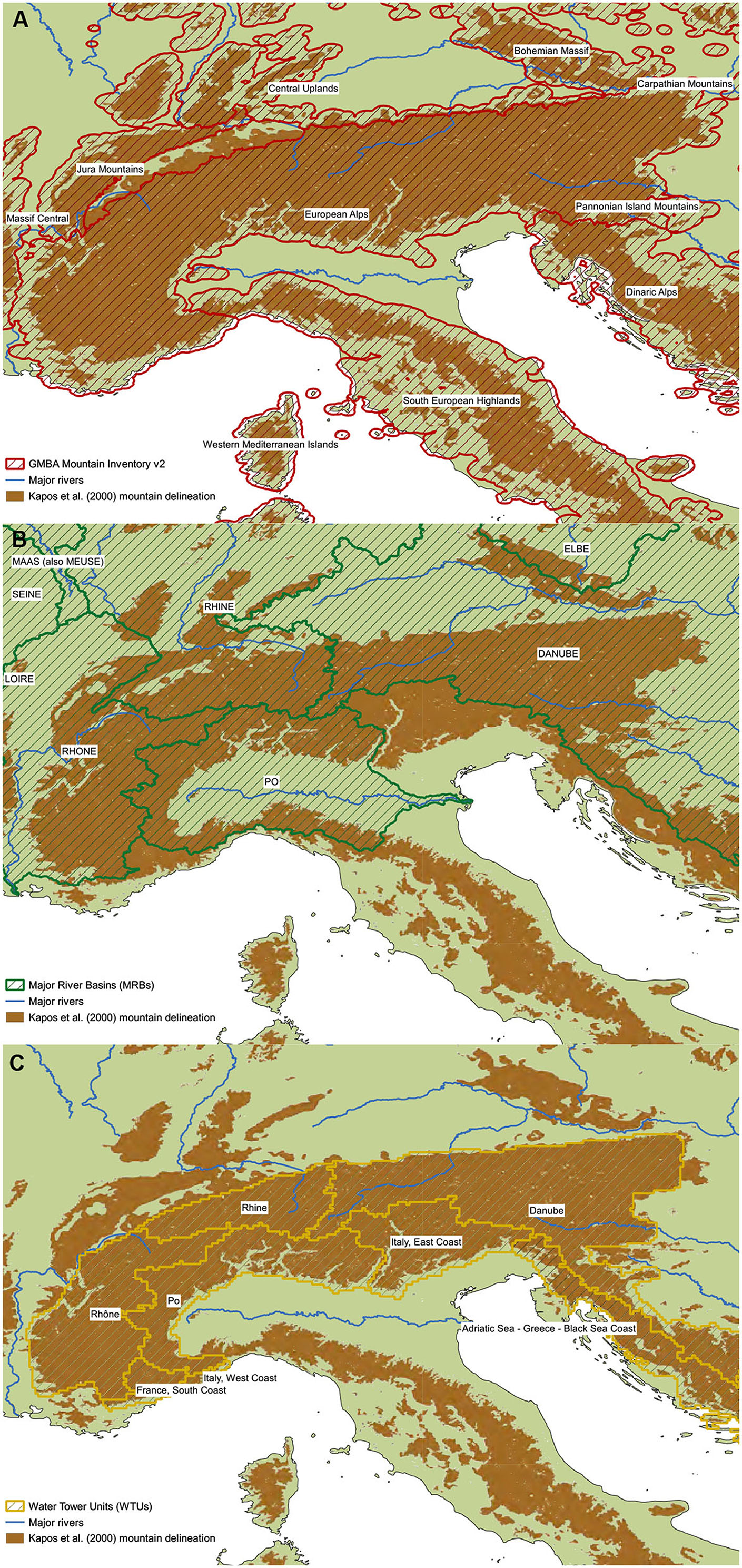
Figure 1. Illustration of the spatial polygon datasets used in this study for aggregation and reporting for a region centered on the European Alps; the GMBA Mountain Inventory v2 (Snethlage et al., 2022a) (A), major river basins (MRBs) (GRDC, 2020) (B), and Water Tower Units (WTUs) (Immerzeel et al., 2020a,b) (C).
The main steps of Phase 1 of the workflow were as follows:
1. Conduct a spatial intersection to identify the mountainous parts of each GMBA Mountain Inventory polygon according to the selected mountain delineation (the results of which are hereafter referred to as “mountainous regions”), and calculate the resultant areal extents;
2. Identify GHCNd stations that fall within the mountainous regions, and assign them with the corresponding GMBA range ID and name attributes;
3. Split the records of each GHCNd station into four separate tables, one for each variable;
4. For each mountainous region and variable, calculate the total number of stations in that region providing records of any length, the mean station density (again irrespective of record length), the mean record start date, the mean record end date, the mean record length, the proportion of stations with “ongoing” records (defined according to whether the last year is 2021), and the proportion of stations possessing a WMO ID (which can be taken as a proxy for instrumental and data quality).
For Phase 2, a script was developed that enables detailed information on the temporal coverage and observation quality for the record of any variable at individual stations to be plotted efficiently. Statistics and plots can also be readily generated for arbitrary temporal subsets. In developing the quality information script, care was taken to distinguish between days on which blank quality flags were accompanied by valid readings (indicating no quality problems) and days on which blank quality flags were accompanied by missing data (i.e., days for which quality information is not applicable, since there are no observations). Whilst the script's capabilities are illustrated using mountainous stations, it is applicable to all GHCNd stations, which extends its potential utility.
The main steps involved in Phase 3 were as follows:
1. For each mountainous region, extract the elevation of each GHCNd station (irrespective of variable and record length) and plot the resultant elevational distributions against the elevation distribution of the corresponding entire region (by extracting all pixel values within each region from the GMTED2010 terrain data);
2. Calculate a TRI raster from GMTED2010, clip it to the mountainous parts of each MRB, and calculate the approximate mean roughness for each resultant polygon;
3. Conduct a spatial intersection between the additional polygon datasets (MRBs and WTUs) and the “K1” mountain delineation to identify the mountainous zones of each MRB and WTU polygon;
4. Calculate the mean station density, again irrespective of variable and record length, within each of the resultant mountain regions (i.e., the WTU polygons and the mountainous parts of the MRB polygons);
5. Calculate the sum of the human population and sum of GDP across the entire MRB polygons; and,
6. Relate mean mountain station densities (by MRB and WTU) to the corresponding derived population, GDP, and WTI metrics.
Figure 2 shows the locations of all mountain stations in the GHCNd inventory (i.e., stations falling within both “K1” and a named GMBA mountain range) that provide data for any of the four variables, for any time period. One observes that the spatial distribution of stations is highly uneven (or clustered), with a large number in the mountains of North America, eastern South America, Southern Africa, and Scandinavia, for instance. Station density appears much lower in the west of South America, the remainder of Africa, and parts of the Middle East and Asia.
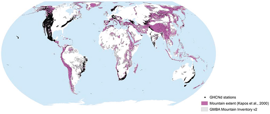
Figure 2. Spatial distribution of GHCNd stations in mountainous terrain (i.e., stations that fall within both the mountain delineation used and one of the GMBA Mountain Inventory polygons) providing measurements of at least one of the four variables—TMIN, TMAX, PRCP, or SNWD—irrespective of record length.
Figure 3 shows mean mountain station density per 1,000 km2 for PRCP (A), TMAX (B), and SNWD (C), again irrespective of record length, by GMBA mountain range. Figures 4–6, meanwhile, show mean record length, mean record start date, and mean record end date for the same three variables, respectively. The corresponding maps for TMIN are provided in the online Supplementary Materials. Figure 3 reveals that in a given mountain region, there are often more precipitation than temperature stations (i.e., the mean spatial density for TMAX is often lower than that of PRCP).
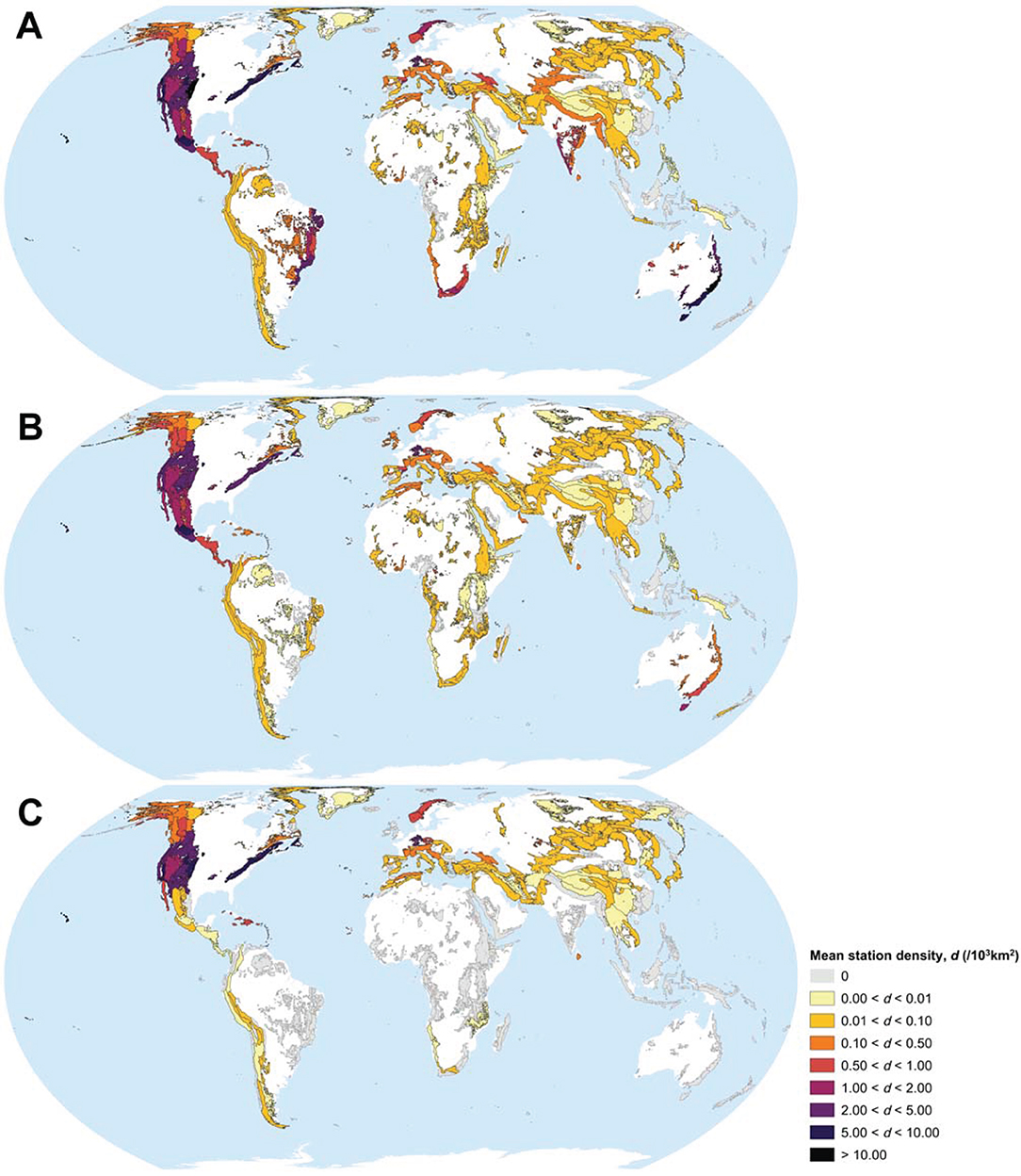
Figure 3. Mean spatial density of GHCNd stations in mountainous terrain for PRCP (A), TMAX (B), and SNWD (C) by GMBA mountain polygon, irrespective of record length. The corresponding plot for TMIN is provided in the online Supplementary Material. Whilst the entire GMBA regions are shown, the statistics plotted correspond to only the mountainous parts of these regions, as delineated by Kapos et al. (2000).
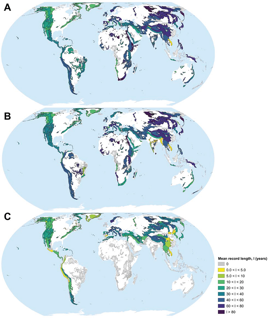
Figure 4. Mean approximate record length of GHCNd stations in mountainous terrain for PRCP (A), TMAX (B), and SNWD (C) by GMBA mountain polygon. The corresponding plot for TMIN is provided in the online Supplementary Material. Whilst the entire GMBA regions are shown, the statistics plotted correspond to only the mountainous parts of these regions, as delineated by Kapos et al. (2000).
For all three variables, station density is exceptionally high in North America. There are also several mountainous regions in which there are no stations whatsoever. That this is noticeably more common for SNWD probably simply reflects lower or negligible regular snow accumulations and/or the limited societal importance of snow in warmer climatic zones. It is slightly surprising, however, that there are very few stations in the inventory providing snow measurements in East Africa, and none whatsoever in Himalaya or Australasia.
Figure 4 represents the indicative mean record length per mountain region. In some contrast to the patterns of spatial density (Figure 3), it shows that many of the mountain regions with the longest records are located in Africa, Central Asia, Siberia and East Asia; in North America, mean record lengths are generally shorter, although they are longer for TMAX than for PRCP. Across most regions where snow stations are present, the corresponding mean SNWD record lengths are shorter than those for the other variables.
Figures 5, 6 simply represent the mean record start and end dates from which the mean record lengths (Figure 4) were calculated. Notable features of Figure 5 are that precipitation records began earliest in parts of Africa, Europe, and Asia, and that initiation was also fairly early in Siberia. TMAX records likewise began relatively early on in Siberia. The average onset of SNWD observations occurred at a broadly similar time in many global mountain regions. Figure 6 reveals that the mean station end date for mountain records across many ranges falls in the second half of the twentieth century. In other words, many stations records have now ended. This is especially the case for PRCP in the European Alps and Himalaya, and to a lesser extent North America. Many TMAX and SNWD are also seen to have already ended in North America. The spatial data from which these plots were generated are provided in the online Supplementary Material. Using these data, the individual mountain regions with the highest station densities and longest record lengths for a given variable can be rapidly identified, as can those with few or no stations, or only very short records. In addition, the proportion of stations in each mountainous region which possess a WMO ID—a proxy for station and observation quality and standards—is also provided as an attribute of the supplementary spatial datasets (these results are not presented here).
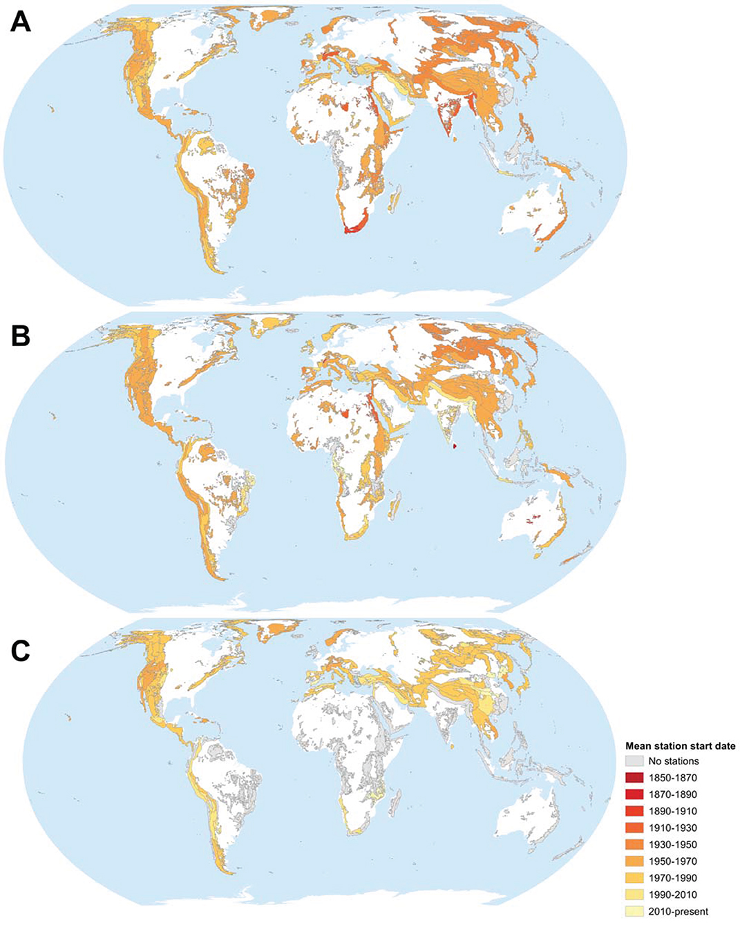
Figure 5. Mean record start date of GHCNd stations in mountainous terrain for PRCP (A), TMAX (B), and SNWD (C) by GMBA mountain polygon. The corresponding plot for TMIN is provided in the online Supplementary Material. Whilst the entire GMBA regions are shown, the statistics plotted correspond to only the mountainous parts of these regions, as delineated by Kapos et al. (2000).
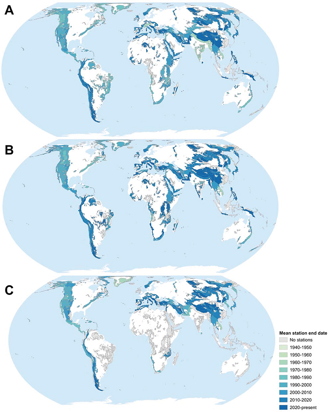
Figure 6. Mean record end date of GHCNd stations in mountainous terrain for PRCP (A), TMAX (B), and SNWD (C) by GMBA mountain polygon. The corresponding plot for TMIN is provided in the online Supplementary Material. Whilst the entire GMBA regions are shown, the statistics plotted correspond to only the mountainous parts of these regions, as delineated by Kapos et al. (2000).
Figure 7 exemplifies the capabilities of the script that was developed to provide a more detailed assessment of temporal coverage at an individual station. Specifically, the plots provide a quantification of the relative frequencies of observed vs. missing data for a given variable at that station (Figure 7A), and full information on data availability with respect to time for multiple variables at a given station (Figure 7B). In this example, one observes that although the total record length (in the sense of end minus start date) is relatively long, the proportion of missing data in the intervening period is considerable. In addition, the proportion of missing data is inconsistent across variables; there being particularly few SNWD observations here.
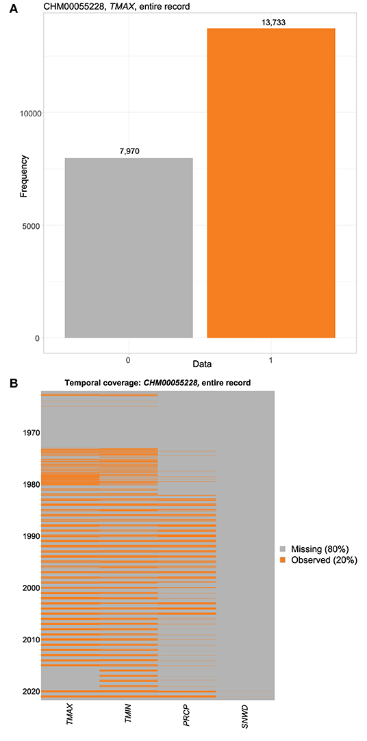
Figure 7. Examples of temporal coverage plots generated using the script developed. Frequency of observations vs. missing data for a particular variable TMAX at a given station (CHM00055228) (A), and an illustration of observations vs. missing data on a daily basis at the same station for all core variables (B). The percentages correspond to the integrated proportion of observed to missing data across the four variables for their combined maximum record length. The script also enables users to make arbitrary temporal subsets of any data record.
Figure 8 illustrates a further capability of the script; namely its capacity to summarize the associated quality information (QFLAG) for a given GHCNd station and variable of interest. At this example station, for TMIN, one observes that there are very few records with quality issues. One additionally observes that this record is hardly afflicted by any missing data.
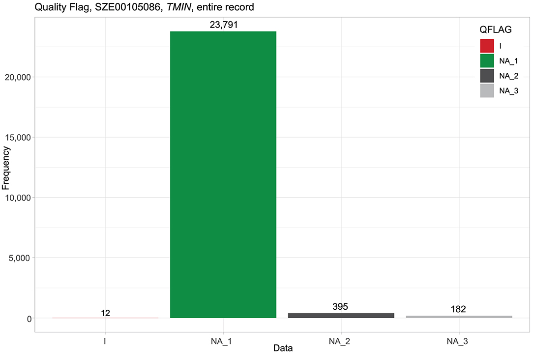
Figure 8. Example data quality plot for station SZE00105086 generated using the script developed. NA_1 means that there is a real (i.e., non-NA) value in for the corresponding observation, and so a blank quality flag (QFLAG) entry indicates no quality problems, NA_2 means that a given day was present in the original file but there was no valid observation (i.e., observation was NA), and NA_3 denotes records for days between the first and last records that were not present in the original file, and for which NAs were inserted (i.e., the record was “padded” to produce a continuous time stamp column). “I” indicates “failed internal consistency check”. For a full list of possible quality flags, see the GHCNd metadata information (“readme.txt”). The script also enables users to make arbitrary temporal subsets of any data record.
Importantly, the script can be applied to provide summary information for any desired GHCNd station and variable combination (including those stations located outside of mountain regions, and those variables not considered in this study), either for the entire record periods or over any temporal subsets of interest.
Figure 9 presents, for selected mountain regions, the elevational coverage of GHCNd stations relative to the underlying elevational distribution, or hypsometry, according to a relatively high resolution Digital Terrain Model (DTM). As such, this approach enables those regions whose elevational distributions (and especially the higher elevations) are comparatively under-sampled by the in situ station network to be easily identified. One observes that the elevational coverage of GHCNd is especially limited—that is, higher elevations are under-sampled—in ranges such as the Caucasus Mountains, the Cordillera Occidental (Central Andes), the Dry Andes, the Mongolian Altai, Himalaya, the Hindu Kush, the Pamir Mountains, and Tian Shan. Plots for all 292 mountain regions are provided in the online Supplementary Material.
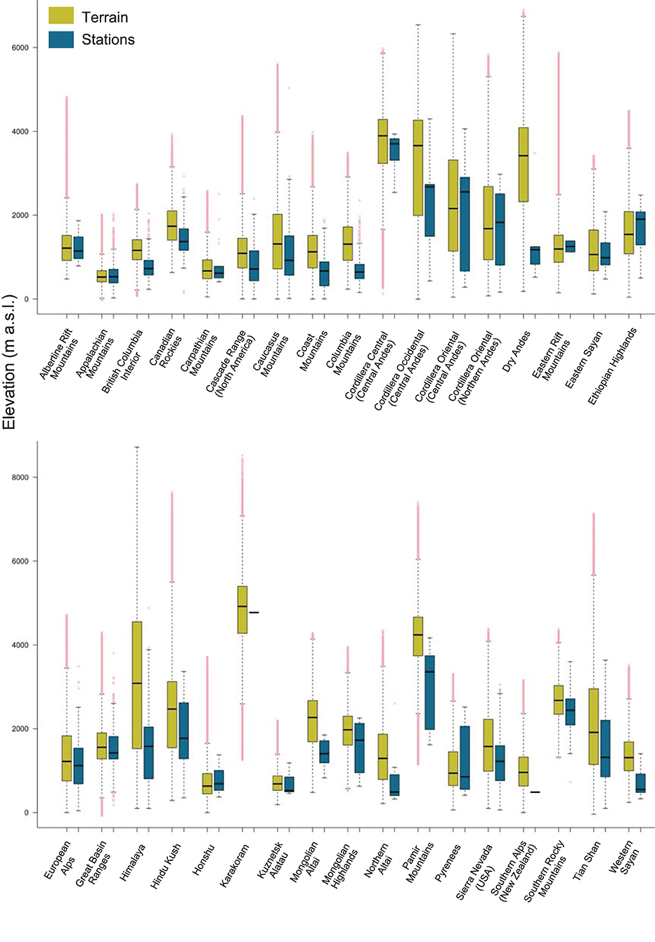
Figure 9. Elevational coverage of GHCNd stations irrespective of variable or record length of the mountainous parts of 34 selected GMBA polygons relative to the underlying elevation distribution of those regions. Plots for all regions are provided in the online Supplementary Material.
Figures 10, 11 present scatter plots that were developed by extracting the potential co-variate data according to the MRB reporting geometries. Figure 10 shows mean GHCNd station density against mean TRI across the mountainous parts (i.e., area within “K1”) of each MRB. It reveals that for low TRI values, there is some tendency for mean station density to increase with increasing ruggedness. This suggests that the need for a higher density of stations to provide a certain benchmark degree of climate data representativeness in areas with more complex topography compared with flatter ones may be at least partially recognized in monitoring network design. However, with increasing TRI beyond approximately 80, mean station density generally declines sharply which may indicate that practical constraints become more dominant in extremely rugged terrain. Some pattern by continent is present, although the grouping is not strong.
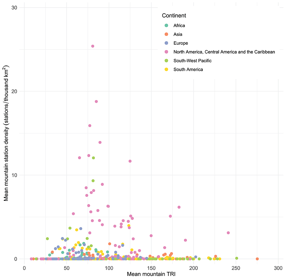
Figure 10. Mean mountain GHCNd station density, irrespective of variable and record length, against mean mountain Terrain Ruggedness Index (TRI) of the mountainous part of each Major River Basin (MRB).
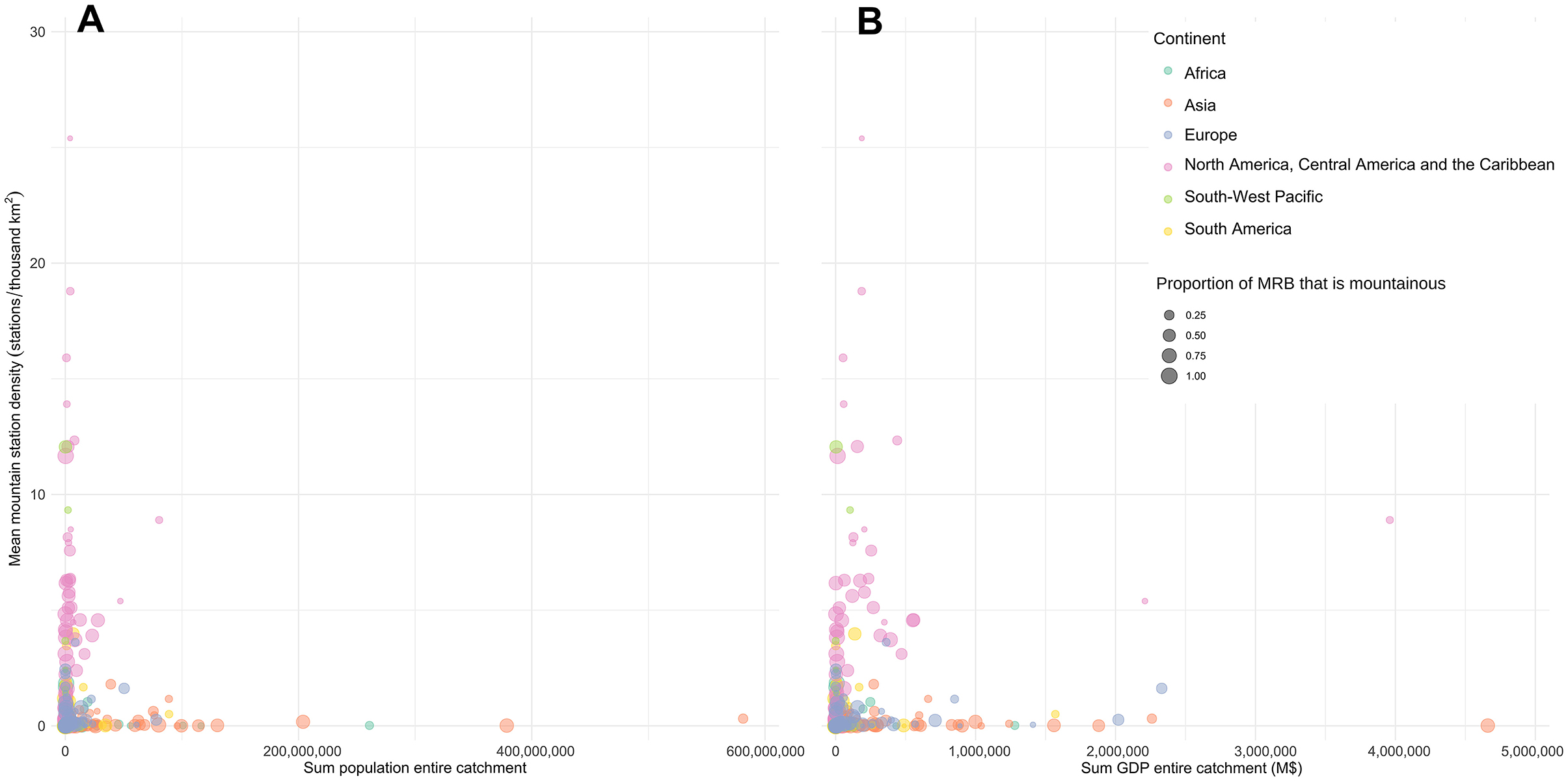
Figure 11. Mean mountain GHCNd station density, irrespective of variable and record length, against the total human population of the associated downstream catchment (A) and the total Gross Domestic Product (GDP) of the associated downstream catchment (B), for each Major River Basin (MRB).
Figures 11A,B, meanwhile, show mean mountain station density against the sum of the 2015 human population and the sum of 2015 GDP across the entireties of their corresponding river basins, respectively. Dot size reflects the proportion of each MRB that is mountainous. Perhaps somewhat surprisingly given the known importance of flows of mountain goods and services to downstream populations, Figure 11A reveals that there is very little overall association between mean station density and the sum of the population in the corresponding catchment. Stronger grouping by continent is apparent, however, with station densities being especially high with respect to catchment populations in North and Central America (including in MRBs whose mountainous proportions are only small), and the inverse situation in Asia (including in MRBs whose mountainous proportions are more substantial). The association with GPD in Figure 11B is slightly stronger, although there are clearly also catchments with large economies whose mountain components are little monitored. The grouping by continent is broadly similar to that in Figure 11A.
It would seem that that wider political and economic factors (e.g., national GDP), via their influence on investment decisions around environmental monitoring, have a stronger influence on the spatial patterns of in situ climatological monitoring in mountains than more objective or hypothetical considerations. It may therefore be concluded that in many regions, the station network (as represented by the GHCNd inventory) may be some way off being “optimized” in these terms.
Figure 12 shows the association between the mean density of GHCNd stations within mountainous parts of the WTUs and each WTI. The relationship is relatively weak, with many WTUs with high WTI values being associated with modest or low station densities. Again, a clear continental signature is evident. Perhaps most notably, the three WTUs that have been identified as holding the highest hydrological importance—the Amu Darya, Tarim Interior, and Indus (Immerzeel et al., 2020a), see also (Kaser et al., 2010)—have extremely low station densities. These regions should arguably be treated as priorities for initiatives to improve in situ data coverage (and work should be undertaken to ensure the inclusion of any existing stations in global inventories such as GHCNd).
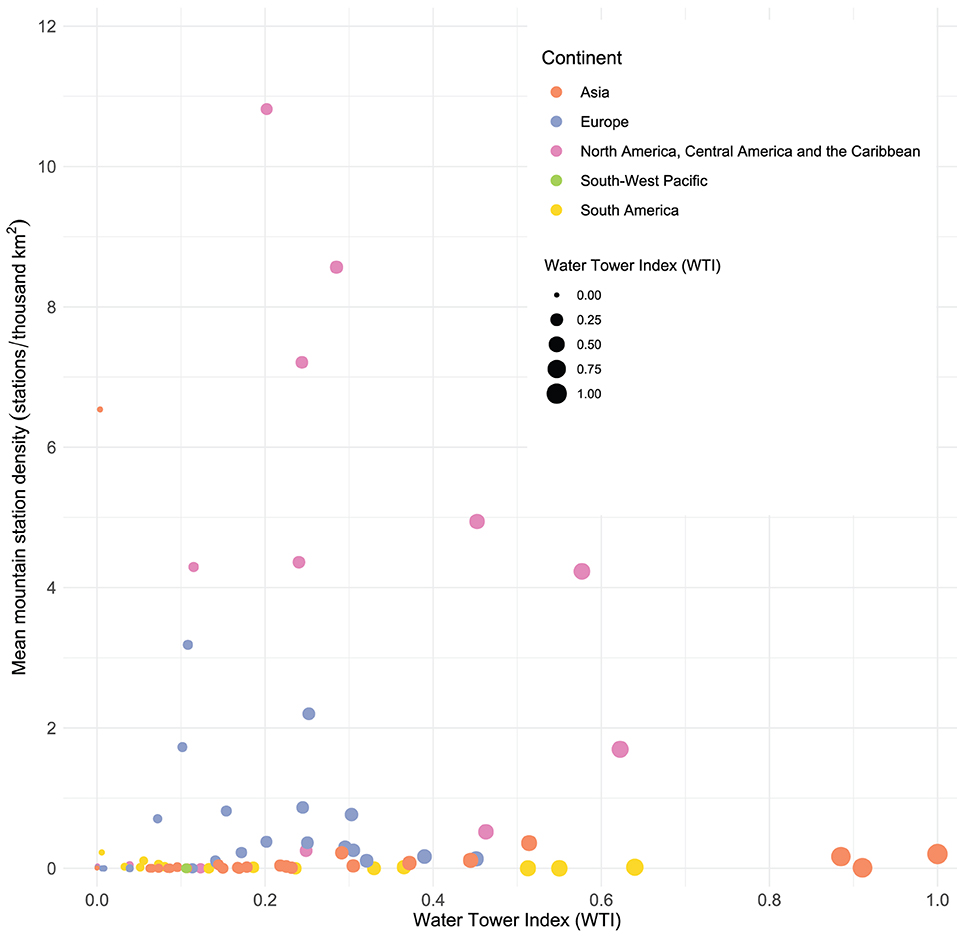
Figure 12. Mean mountain GHCNd station density for each Water Tower Unit (WTU) against that WTU's Water Tower Index (WTI).
The observation that many mountain records have now ended, i.e., that in situ data coverage has begun to diminish over recent decades, is known to be broadly mirrored in non-mountainous regions. Whilst the associated data loss may be partially offset or even justified by advancements in remote sensing, it is clear that, in mountainous terrain especially, in situ observations remain critical (Thornton et al., 2021b). Efforts should therefore be made to re-activate some of these stations where possible. In summary, the various spatial, temporal, and elevational patterns of in situ mountain climatological data presented above can likely only be explained by a complex combination of possible pre-defined “ideals” and various broader historical, geographical, political, financial, and technical factors.
Spatial “gaps” in the coverage of GHNCd stations (Figure 1) do not necessarily indicate a complete absence of climatological observations. Firstly, it is likely that not all stations operated by National Hydrological and Meteorological Services (NHMSs) are integrated into global databases such as GHCN. For instance, Condom et al. (2020) reported that national databases of several Andean countries were only partly integrated with international ones, with much variability from one country to the next. It is also known that many mountain stations from Russia and Central Asia are not integrated. Whist these omissions must certainly be borne in mind when interpreting our findings, we are confident that they are nevertheless broadly representative on a global scale. Still, in case there are major differences with the GHCN, it could be useful to conduct a similar analysis on the operational stations represented in the WMO's OSCAR (surface) database.
More broadly, we recommend that NHMSs and other state agencies with environmental monitoring responsibilities to their utmost to ensure that all of their stations are integrated into the relevant global inventories, and that the metadata are as correct and current as possible. Coverage analyses on these more comprehensive inventories would likely be even more informative; as it is, whilst numerous interesting patterns can be detected, reaching definitive conclusions is challenging given the strong likelihood that some (and in certain regions perhaps many) operational stations are not represented in GHCNd. Where possible, it could also provide useful for the organizations that curate such inventories to interact more with one another such that summaries or comparisons of the respective inventories' scopes, similarities, and differences (e.g., in terms of station inclusion criteria) can be better communicated to potential users. Moreover, other inventories should follow the excellent example of GHCNd by providing access to the historical time-series themselves where possible, which would facilitate detailed temporal coverage analyses like those presented here.
It is also crucial to emphasize that many climatological observations in mountainous areas are made not by operational services or organizations, but rather by research-oriented groups. These sites often provide extremely valuable data in some of the world's most remote and inhospitable regions. However, the stations and their corresponding observations may not currently feed into the more operationally-focused inventories. This could be due to factors such as limited time and capacity, or because the observations may not necessarily always conform to the rigid and consistent observational protocols and quality assurance standards that operation stations are more often able to attain. As such, in considering exclusively the stations of the GHCNd database, this analysis has likely overlooked many other sources of available data that could improve the picture of mountain data coverage somewhat (e.g., locally, or with respect to specific variables and/or time periods). Our approach is defensible, however, because simply discovering the existence of many such stations across the world's mountains, obtaining consistent and reliable metadata information, and accessing their associated data records, can all be extremely challenging and time-consuming tasks. Our analysis has also been limited to a small number of climatological variables (although generally some of the most important) present in GHCN. However, many applications require more diverse, interdisciplinary sets of variables to be monitored (Thornton et al., 2021b).
With precisely these considerations in mind, the Global Network for Observations and Information in Mountain Environments (GEO Mountains) has recently released the first version of its Inventory of In Situ Mountain Observational Infrastructure (GEO Mountains, 2021). This resource seeks to be more interdisciplinary and research station or site-oriented, and should enable users to develop a more comprehensive and integrated view of which variables are being measured using in situ techniques, where, by whom, in what fashion (instrumentation, protocols, etc.), and over what time periods in mountain regions globally—thereby filling the gap identified by Shahgedanova et al. (2021). The inventory also seeks to facilitate access to the corresponding data by providing links to the repositories from which downloads can be made, where the organizations or individuals involved make their data available. Contributions have been invited from the community to either improve the information that has already been captured on existing sites, or else provide information on sites that are currently missing. Updated versions of the inventory will be released regularly. Ultimately, once sufficiently populated, it is hoped that the inventory will support a similar but more holistic data coverage analysis to the purely climatological one presented here. This could include, for instance, a comprehensive assessment of the extent to which the data requirements associated with a recently proposed set of so-called Essential Mountain Climate Variables (EMCVs) (Thornton et al., 2021b) can presently be met (and therefore where the major remaining gaps lie). In this sense, the present study has illustrated the type and breadth of metadata (and associated data) that the inventory must capture if such an extended mountain data coverage or gap analysis is to be achievable and insightful. As a point of comparison, the ILTER's DEIMS-SDR system (Wohner et al., 2019) provides excellent and consistent foundational information about each site belonging to the network, but does not consistently provide all the metadata that would be need to conduct an analysis such as that presented here (e.g., for assessing temporal coverage in detail).
A fundamental challenge associated with the use of in situ data in mountains especially is that the information they provide may be of limited spatial representativeness away from measurement locations, and/or informativeness in terms of finer scale micro-climate, Strachan et al. (2016). A need therefore exists to not only actually increase the number of station data available (e.g., to allow better independent evaluation of gridded climate products), but also generate more optimally integrated in situ measurements, remotely-sensed data, and numerical models (Thornton et al., 2021b). With this in mind, GEO Mountains has also recently released the first version of its General Inventory to complement its in situ inventory (GEO Mountains, 2022). This resource lists and provides links to available remotely sensed and modeled datasets. Again, a crowd-sourced approach is being taken to populate it. Once further developed, by jointly considering the two inventories it will hopefully be possible to identify a global network of so-called “Mountain Observatories”, i.e., mountain regions with a high density of long term measurements pertaining to a wide range of interdisciplinary variables obtained using a variety of approaches (Shahgedanova et al., 2021). The recent ratification of the WMO's Unified Data Policy Resolution (Res.1) should help further enhance the free and open exchange of a wide range of observational data from the world's mountain regions in support of such tasks. Within this framework, progress can also be expected on issues related to financing, capacity and technology, and removing any persistent cost or legal barriers (whilst simultaneously fully acknowledging and protecting the rights of data providers). Over time, station inventories containing nationally-run operational stations and more research-oriented stations should become more interoperable, with a single, integrated inventory being a possible eventual goal.
In the scope of this work, we did not quantify record intermittency or proportion of gaps within the recorded period at all stations. However, this would be theoretically possible using the scripts provided. Doing so could provide greater insight into spatial and temporal patterns in aspects related to instrumentation quality, maintenance, and the technical and institutional capacities of those responsible for in situ climatological monitoring (Strachan et al., 2016). Differences in the extents to which monitoring operations are affected by extreme weather conditions across the world's mountainous region may also emerge. More technical challenges, related for instance to biases in the fundamental measurements—for example biases in solid precipitation quantification associated with gauge undercatch (Kochendorfer et al., 2021), understanding the impacts of station siting on spatial representativeness, or challenges associated with reliable data transmission in challenging terrain should also be considered more fully in future work. Such issues may not be routinely reflected in the observational quality information provided, which could partially explain why precipitation undercatch, for instance, is still not routinely accounted for in interpolated gridded precipitation products. Nevertheless, more sophisticated data imputation methods to fill gaps in in situ records are emerging (Tang et al., 2021; Thornton et al., 2021c).
With respect to the more relative component of our coverage analysis, it must be highlighted that a range of other potential factors, including the nature of typical local weather patterns, accessibility, propensity to natural hazards, and so forth would also influence the hypothetical “optimal” configuration or distribution of station networks in a particular mountainous region. Including these factors fell beyond the scope of the present work, but again could be explored in future. Similarly, assessing climatological data coverage relative to other important ecosystem goods and services that mountain regions contribute to society (e.g., timber production, energy production, biodiversity maintenance, tourism and recreation etc.) could be another potential avenue, although the associations are likely to be even weaker than those we presented. In summary, the metrics considered here are arguably not the only ones that should be taken into account when determining priority regions and variables for new long-term measurement campaigns. Both outstanding scientific questions and the needs of local populations (currently and under future scenarios) should be taken into account.
Similar analysis could be attempted using hydrological gauging stations. However, careful consideration would have to be give to the choice of spatial coverage metric employed. This is because individual stations on larger watercourses some distance from headwaters will cover large mountainous catchments, but will inherently integrate a considerable amount of spatial and temporal variability. Conversely, whilst stations at the outlet of first-order catchments provide very specific information related to those catchments, not all headwaters can be monitored for practical reasons. Therefore, a hypothetical mountain river discharge monitoring network at the mountain range scale should arguably span a range of catchment sizes (potentially nested) in addition to topographic, climatological, and geological conditions. Anthropogenic interventions (e.g., extractions, reservoirs, etc.) should also be monitored. By introducing other datasets and distributed, physically-based numerical models that can represent all key processes and their interactions (e.g., bidirectional groundwater-surface water interactions) explicitly in time and space (e.g., Thornton et al., 2022), there is an increasingly realistic prospect of being able to fill the gaps between observations (not only for discharge, but other variables too) in a reasonable fashion.
It could be informative to repeat the analyses fairly regularly, for example every year or few years, in order to capture changes in data coverage through time. Given the scripted workflow, this would be feasible. In this way, it may even be possible to intervene to address any issues before the long-term continuance of records is significantly compromised. Finally, similar questions related to data gaps and user data needs can also be addressed from a more qualitative or heuristic perspective, for example via stakeholder engagement and surveys. For example, GEO Mountains is currently undertaking a series of regional consultations on these topics.
This study has presented a simple but much-needed assessment of the absolute and relative coverage of in situ climatological time-series data in the world's mountain regions according to the GHCNd database. Spatial, temporal, and elevational coverage were explicitly considered for daily frequency records of three critical climate-related variables—near-surface air temperature, precipitation, and snow depth. Prior to this study, only rather general patterns of in situ climatological data coverage in mountains had been identified at a global level, although more extensive information did exist for some more specific regions and variables. Our work therefore elucidates certain key similarities and differences between mountain regions in terms of their climatological data coverage. Although not all operational stations may be included in the global inventory used, we are confident that our results are broadly representative.
Several specific conclusions can be drawn. Firstly, whilst spatial and temporal data coverage varies greatly between mountain regions globally, spatial density and record length appear partially inversely related (e.g., dense but short records in North America, with longer but less dense records in Africa, Asia, and Siberia). Secondly, whilst the elevational range of many important mountainous regions is reasonably well sampled by the GHCNd stations, there is a general tendency toward under-sampling of higher elevations, and in certain regions this is severe. Thirdly, and perhaps slightly surprisingly, we detected only weak associations between mountain station densities on the one hand, and downstream catchment population and economic output on the other; it appears therefore that broader societal drivers (e.g., direct funding and technical capacities at a national level) dominate patterns of mountain climatological monitoring. Lastly, and potentially concerningly, several of the mountain regions identified as being the most hydrologically-important on the planet by Immerzeel et al. (2020a) have the lowest station densities according to GHCNd. It thus appears that the network is far from close to being “optimized” in purely idealized or hypothetical terms.
These findings could help to inform and justify future investment decisions pertaining to the maintenance and installation of in situ infrastructure made in the context of regional and international programmes. Specially, they could help guide the identification of regions, variables, and other aspects in which new stations or networks, more reliable sensors, advanced transmission technologies, and/or enhanced data sharing could be most beneficial.
Our main results are complemented by an open-source script that enable users to plot temporal coverage and quality statistics for any station/variable/temporal subset combination in the GHCNd catalog. The application of our workflow more broadly should allow mountain (and indeed non-mountain) data coverage to be “tracked” more rigorously in near real time. For instance, the entire analysis could be run in an automated fashion to generate reports following major inventory releases or alternatively on a regular basis (e.g., every month or year). It could also be modified to conduct similar analyses on other in situ station networks. In this sense, our study demonstrates the breath of metadata that GEO Mountains' more interdisciplinary Inventory of In Situ Mountain Observational Infrastructure (GEO Mountains, 2021) must capture to make it a suitable basis for conducting similar coverage analyses for a wider range of important environmental variables.
Looking ahead, a clear need exists to integrate station data and metadata from a variety of sources into consistent and comprehensive global inventories. Doing so will greatly improve data re-use, minimize the risks of infrastructural redundancy, and improve data inter-comparability and interoperability. Ultimately, these efforts will help to ensure that any conclusions drawn and subsequent decisions made are as robust as possible, to the benefit of the global community of mountain researchers, practitioners, and policy makers.
The code and input and output datasets associated with this study can be accessed at: doi: 10.5281/zenodo.6081715. Spatial data outputs (.sqlite files) can be easily visualized in QGIS – simply drag and drop.
JMT and CA conceived the analysis. JMT wrote the code, produced all figures, and drafted the text. NP and MS provided support and advice at all stages. All authors contributed to the redaction of the manuscript.
JMT was supported by the Swiss Agency for Development and Cooperation (SDC) under its Adaptation at Altitude Programme (Project Number 7F-10208.01.02) and CA was supported by the Swiss Academy of Sciences (SCNAT) via its support for the Mountain Research Initiative (Project No. FNW0004_004-2019-00).
The authors declare that the research was conducted in the absence of any commercial or financial relationships that could be construed as a potential conflict of interest.
All claims expressed in this article are solely those of the authors and do not necessarily represent those of their affiliated organizations, or those of the publisher, the editors and the reviewers. Any product that may be evaluated in this article, or claim that may be made by its manufacturer, is not guaranteed or endorsed by the publisher.
This study would not have been possible without the dedicated work undertaken at NOAA's National Centers for Environmental Information (NCEI) to compile and maintain the Global Historical Climatology Network (GHCN) database, for which we are extremely grateful. We also thank the developers and maintainers of the other open source data and software used; PostgreSQL 13.1, PostGIS 3.1, PgAdmin 4 v5.0, GDAL 3.0.4, QGIS 3.14.1, and R 4.0.4. Finally, we thank the two reviewers for their helpful comments.
1. ^Thornton, J., Snethlage, M., Sayre, R., Urbach, D., Viviroli, D., Ehrlich, D., et al. [Under review]. Human populations in the world's mountains: spatio-temporal patterns and topo-climatic controls. PLoS ONE.
Adler, C., Wester, P., Bhatt, I., Huggel, C., Insarov, G. E., Morecroft, M.D., et al. (2022). “Cross-chapter paper 5: mountains supplementary material,” in Climate Change 2022: Impacts, Adaptation, and Vulnerability. Contribution of Working Group II to the Sixth Assessment Report of the Intergovernmental Panel on Climate Change, eds H. -O. Pörtner, D. C. Roberts, M. Tignor, E. S. Poloczanska, K. Mintenbeck, A. Alegría, M. Craig, S. Langsdorf, S. Löschke, V. Möller, A. Okem, and B. Rama. Available online at: https://www.ipcc.ch/report/ar6/wg2/
Bales, R. C., Molotch, N. P., Painter, T. H., Dettinger, M. D., Rice, R., and Dozier, J. (2006). Mountain hydrology of the western United States. Water Resour. Res. 42, 1–13. doi: 10.1029/2005WR004387
CH2018 (2018). CH2018-Climate Scenarios for Switzerland: Technical Report. Technical report, Zurich.
Climate Research Unit (2021). CRUTEM4 Temperature station data. Available online at: https://crudata.uea.ac.uk/cru/data/temperature/
Condom, T., Martínez, R., Pabón, J. D., Costa, F., Pineda, L., Nieto, J. J., et al. (2020). Climatological and hydrological observations for the South American andes: in situ stations, satellite, and reanalysis data sets. Front. Earth Science, 8, 92. doi: 10.3389/feart.2020.00092
Danielson, J., and Gesch, D. (2011). Global Multi-resolution Terrain Elevation Data 2010 (GMTED2010). U.S. Geological Survey Open-File Report 2011-1073, 2010:26.
Dong, C. (2018). Remote sensing, hydrological modeling and in situ observations in snow cover research: a review. J. Hydrol. 561, 573–583. doi: 10.1016/j.jhydrol.2018.04.027
Gärtner-Roer, I., Nussbaumer, S. U., Hüsler, F., and Zemp, M. (2019). Worldwide assessment of national glacier monitoring and future perspectives. Mt Res. Dev. 39, A1–A11. doi: 10.1659/MRD-JOURNAL-D-19-00021.1
GEO Mountains (2021). Inventory of In Situ Mountain Observational Infrastructure, v1.0. figshare. doi: 10.6084/m9.figshare.14899845.v1
GRDC (2020). Major River Basins of the World. Available online at: https://www.bafg.de/GRDC/EN/02_srvcs/22_gslrs/221_MRB/riverbasins_node.html
Harris, I., Osborn, T. J., Jones, P., and Lister, D. (2020). Version 4 of the CRU TS monthly high-resolution gridded multivariate climate dataset. Sci. Data 7, 109. doi: 10.1038/s41597-020-0453-3
Hock, R., Rasul, G., Adler, C., Cáceres, B., Gruber, S., Hirabayashi, Y., et al. (2019). “High mountain areas,” in IPCC Special Report on the Ocean and Cryosphere in a Changing Climate, Chapter 2, eds H.-O. Pörtner, D. Roberts, V. Masson-Delmotte, P. Zhai, M. Tignor, E. Poloczanska, K. Mintenbeck, A. Alegría, M. Nicolai, A. Okem, B. Petzold, B. Rama, and N. Weye. (Cambridge; New York, NY: Cambridge University Press). doi: 10.1017/9781009157964.004
Hughes, A. C., Orr, M. C., Ma, K., Costello, M. J., Waller, J., Provoost, P., et al. (2021). Sampling biases shape our view of the natural world. Ecography 44, 1259–1269. doi: 10.1111/ecog.05926
Immerzeel, W. W., Lutz, A. F., Andrade, M., Bahl, A., Biemans, H., Bolch, T., et al. (2020a). Importance and vulnerability of the world's water towers. Nature 577, 364–369. doi: 10.1038/s41586-019-1822-y
Immerzeel, W. W., Lutz, A. F., Andrade, M., Bahl, A., Biemans, H., Bolch, T., et al. (2020b). Supplementary data to: Importance and vulnerability of the world's water towers. doi: 10.5281/zenodo.5993521933
Kapos, V., Rhind, J., Edwards, M., Price, M. F., and Ravilious, C. (2000). Developing a map of the world's mountain forests. Forests in sustainable mountain development: a state of knowledge report for 2000. Task Force on Forests in Sustainable Mountain Development, 4–19.
Kaser, G., Grosshauser, M., and Marzeion, B. (2010). Contribution potential of glaciers to water availability in different climate regimes. Proc. Natl. Acad. Sci. U.S.A. 107, 20223–20227. doi: 10.1073/pnas.1008162107
Kochendorfer, J., Earle, M., Rasmussen, R., Smith, C., Yang, D., Morin, S., et al. (2021). How Well are We Measuring Snow Post-SPICE? Bull. Am. Meteorol. Soc. 103, pp.E370–E388. doi: 10.1175/BAMS-D-20-0228.1
Kohler, T., and Maselli, D., (Eds). (2009). Mountains and Climate Change - From Understanding to Action. Bern: Geographica Bernensia.
Kummu, M., Taka, M., and Guillaume, J. H. (2018). Gridded global datasets for Gross Domestic Product and Human Development Index over 1990-2015. Sci. Data 5, 1–15. doi: 10.1038/sdata.2018.4
Menne, M. J., Durre, I., Vose, R. S., Gleason, B. E., and Houston, T. G. (2012). An overview of the global historical climatology network-daily database. J. Atmosphere. Oceanic Technol. 29, 897–910. doi: 10.1175/JTECH-D-11-00103.1
Morán-Tejeda, E., Llorente-Pinto, J. M., Ceballos-Barbancho, A., Tomás-Burguera, M., Azorín-Molina, C., Alonso-González, E., et al. (2021). The significance of monitoring high mountain environments to detect heavy precipitation hotspots: a case study in Gredos, Central Spain. Theor. Appl. Climatol. 146, 1175–1188. doi: 10.1007/s00704-021-03791-x
Pepin, N., Arnone, E., Gobiet, A., Haslinger, K., Kotlarski, S., Notarnicola, C., et al. (2022). Climate changes and their elevational patterns in the mountains of the world. Rev. Geophys. 60:e2020RG000730. doi: 10.1029/2020RG000730
Pepin, N., Deng, H., Zhang, H., Zhang, F., Kang, S., and Yao, T. (2019). An Examination of temperature trends at high elevations across the tibetan plateau: the use of MODIS LST to understand patterns of elevation-dependent warming. J. Geophys. Res. 124, 5738–5756. doi: 10.1029/2018JD029798
Pepin, N. C., and Seidel, D. J. (2005). A global comparison of surface and free-air temperatures at high elevations. J. Geophys. Res. D 110, 1–15. doi: 10.1029/2004JD005047
Pesaresi, M., Florczyk, A., Schiavina, M., Melchiorri, M., and Maffenini, L. (2019). GHS-SMOD R2019A - GHS settlement layers, updated and refined REGIO model 2014 in application to GHS-BUILT R2018A and GHS-POP R2019A, multitemporal (1975-1990-2000-2015). Technical report, European Commission, Joint Research Centre (JRC).
Sayre, R., Frye, C., Karagulle, D., Krauer, J., Breyer, S., Aniello, P., et al. (2018). A new high-resolution map of world mountains and an online tool for visualizing and comparing characterizations of global mountain distributions. Mt Res. Dev. 38, 240–249. doi: 10.1659/MRD-JOURNAL-D-17-00107.1
Shahgedanova, M., Adler, C., Gebrekirstos, A., Grau, H. R., Huggel, C., Marchant, R., et al. (2021). Mountain observatories: status and prospects for enhancing and connecting a global community. Mt Res. Dev. 41:A1–A15. doi: 10.1659/MRD-JOURNAL-D-20-00054.1
Snethlage, M. A., Geschke, J., Ranipeta, A., Jetz, W., Yoccoz, N. G., Körner, C., et al. (2022a). A hierarchical inventory of the world's mountains for global comparative mountain science. Sci. Data. 9, 149. doi: 10.1038/s41597-022-01256-y
Snethlage, M. A., Geschke, J., Spehn, E. M., Ranipeta, A., Yoccoz, N. G., Körner, C., et al. (2022b). GMBA Mountain Inventory v2. GMBA-EarthEnv. doi: 10.48601/earthenv-t9k2-1407
Stahl, K., Moore, R. D., Floyer, J. A., Asplin, M. G., and McKendry, I. G. (2006). Comparison of approaches for spatial interpolation of daily air temperature in a large region with complex topography and highly variable station density. Agric. Forest Meteorol. 139, 224–236. doi: 10.1016/j.agrformet.2006.07.004
Strachan, S., Kelsey, E. P., Brown, R. F., Dascalu, S., Harris, F., Kent, G., et al. (2016). Filling the data gaps in mountain climate observatories through advanced technology, refined instrument siting, and a focus on gradients. Mt Res. Dev. 36, 518–527. doi: 10.1659/MRD-JOURNAL-D-16-00028.1
Sun, Q., Zhang, X., Zwiers, F., Westra, S., and Alexander, L. V. (2021). A Global, continental, and regional analysis of changes in extreme precipitation. J. Clim. 34, 243–258. doi: 10.1175/JCLI-D-19-0892.1
Tang, G., Clark, M. P., and Papalexiou, S. M. (2021). SC-Earth: a station-based serially complete earth dataset from 1950 to 2019. J. Clim. 34, 6493–6511. doi: 10.1175/JCLI-D-21-0067.1
Thornton, J. M., Brauchli, T., Mariethoz, G., and Brunner, P. (2021a). Efficient multi-objective calibration and uncertainty analysis of distributed snow simulations in rugged alpine terrain. J. Hydrol. 598, 126241. doi: 10.1016/j.jhydrol.2021.126241
Thornton, J. M., Palazzi, E., Pepin, N. C., Cristofanelli, P., Essery, R., Kotlarski, S., et al. (2021b). Toward a definition of essential mountain climate variables. One Earth 4, 805–827. doi: 10.1016/j.oneear.2021.05.005
Thornton, J. M., Therrien, R., Mariethoz, G., Linde, N., and Brunner, P. (2022). Simulating fully-integrated hydrological dynamics in complex Alpine headwaters: potential and challenges. Water Resources Research. 54. doi: 10.1029/2020WR029390
Thornton, P. E., Shrestha, R., Thornton, M., Kao, S.-C., Wei, Y., and Wilson, B. E. (2021c). Gridded daily weather data for North America with comprehensive uncertainty quantification. Sci. Data 8, 190. doi: 10.1038/s41597-021-00973-0
Viviroli, D., Kummu, M., Meybeck, M., Kallio, M., and Wada, Y. (2020). Increasing dependence of lowland populations on mountain water resources. Nat. Sustain. 3, 917–928. doi: 10.1038/s41893-020-0559-9
Wan, H., Zhang, X., Zwiers, F. W., and Shiogama, H. (2013). Effect of data coverage on the estimation of mean and variability of precipitation at global and regional scales. J. Geophys. Res. Atmos. 118, 534–546. doi: 10.1002/jgrd.50118
Wang, X., Pang, G., and Yang, M. (2018). Precipitation over the tibetan plateau during recent decades: a review based on observations and simulations. Int. J. Climatol. 38, 1116–1131. doi: 10.1002/joc.5246
Wohner, C., Ohnemus, T., Zacharias, S., Mollenhauer, H., Ellis, E. C., Klug, H., et al. (2021). Assessing the biogeographical and socio-ecological representativeness of the ILTER site network. Ecol. Indic. 127, 107785. doi: 10.1016/j.ecolind.2021.107785
Wohner, C., Peterseil, J., Poursanidis, D., Kliment, T., Wilson, M., Mirtl, M., et al. (2019). DEIMS-SDR – A web portal to document research sites and their associated data. Ecol. Inform. 51, 15–24. doi: 10.1016/j.ecoinf.2019.01.005
Zandler, H., Haag, I., and Samimi, C. (2019). Evaluation needs and temporal performance differences of gridded precipitation products in peripheral mountain regions. Sci. Rep. 9, 1–15. doi: 10.1038/s41598-019-51666-z
Keywords: climate change, ground-based monitoring, data coverage, mountains, GEO Mountains, water towers
Citation: Thornton JM, Pepin N, Shahgedanova M and Adler C (2022) Coverage of In Situ Climatological Observations in the World's Mountains. Front. Clim. 4:814181. doi: 10.3389/fclim.2022.814181
Received: 12 November 2021; Accepted: 24 February 2022;
Published: 26 April 2022.
Edited by:
Hari Prasad Dasari, King Abdullah University of Science and Technology, Saudi ArabiaReviewed by:
Raju Attada, Indian Institute of Science Education and Research Mohali, IndiaCopyright © 2022 Thornton, Pepin, Shahgedanova and Adler. This is an open-access article distributed under the terms of the Creative Commons Attribution License (CC BY). The use, distribution or reproduction in other forums is permitted, provided the original author(s) and the copyright owner(s) are credited and that the original publication in this journal is cited, in accordance with accepted academic practice. No use, distribution or reproduction is permitted which does not comply with these terms.
*Correspondence: James M. Thornton, amFtZXMudGhvcm50b25AdW5pYmUuY2g=
Disclaimer: All claims expressed in this article are solely those of the authors and do not necessarily represent those of their affiliated organizations, or those of the publisher, the editors and the reviewers. Any product that may be evaluated in this article or claim that may be made by its manufacturer is not guaranteed or endorsed by the publisher.
Research integrity at Frontiers
Learn more about the work of our research integrity team to safeguard the quality of each article we publish.