 Shuai Hu
 Bo Wu
Bo Wu Tianjun Zhou
95% of researchers rate our articles as excellent or good
Learn more about the work of our research integrity team to safeguard the quality of each article we publish.
Find out more
ORIGINAL RESEARCH article
Front. Clim. , 06 January 2023
Sec. Predictions and Projections
Volume 4 - 2022 | https://doi.org/10.3389/fclim.2022.1082026
This article is part of the Research Topic Insights in Predictions and Projections: 2022 View all 7 articles
Indian Ocean dipole (IOD) is one of the dominant modes of interannual variability in the Indian Ocean, which has global climate impacts and thus is one of the key targets of seasonal predictions. In this study, based on a century-long seasonal hindcast experiment from the Coupled Seasonal Forecasts of the 20th century (CSF-20C), we show that the prediction skill for IOD exhibits remarkable decadal variations, with low skill in the early-to-mid 20th century but high skill in the second half of the 20th century. The decadal variations of prediction skills for IOD are caused by two factors. The first is associated with the decadal variation of the ENSO-IOD relationship. Although individual members of the predictions can simulate the variation of the ENSO-IOD relationship, with amplitude close to that in the observation, the feature is greatly suppressed in the ensemble mean due to the asynchrony of variation phases among individual members. In the ensemble mean, the IOD evolution shows an unrealistic stable and high correlation with ENSO evolution. This causes the prediction to have much higher skill for those periods during which IOD is accompanied by ENSO in the observation. The second factor is associated with the decadal variation of IOD predictability in the prediction system. In the prediction system, the decadal variation of IOD signal strength closely follows that of ENSO signal strength. Meanwhile, the IOD noise strength shows variations opposite to the IOD signal strength. As a result, the signal-to-noise ratio greatly increases in the second half of the 20th century due to the enhancement of the ENSO signal strength, which represents the increase of IOD predictability in the prediction system.
The Indian Ocean dipole mode (IOD), characterized by opposite sea surface temperature anomalies (SSTA) between the eastern and western tropical Indian Ocean, is a coupled air-sea interaction mode in the tropical Indian Ocean analogous to the El Niño–Southern Oscillation (ENSO) in the Pacific (Saji et al., 1999; Webster et al., 1999). The IOD shows a seasonally dependent feature, usually forming in boreal summer, peaking in the following autumn, and decaying in the subsequent winter (Li et al., 2003). The IOD can influence global climate through atmospheric teleconnections, such as the Indian Ocean monsoon (Ashok et al., 2001; Ummenhofer et al., 2009; Cai et al., 2011), the South African climate (Black, 2005), the East Asian monsoon (Guan and Yamagata, 2003; Qiu et al., 2014; Doi et al., 2020), the El Niño–Southern Oscillation (ENSO) (Annamalai et al., 2005; Izumo et al., 2010; Luo et al., 2010), and the Antarctic sea ice (Nuncio and Yuan, 2015).
IOD formation is associated with ENSO remote forcing (Baquero-Bernal et al., 2002; Yu and Lau, 2004; Behera et al., 2006; Stuecker et al., 2017). During the El Niño developing summer and autumn, the weakened and eastward shifted Walker circulations tend to suppress the deep convection over the southeastern tropical Indian Ocean, and further drive the alongshore southeasterly wind anomalies off the Sumatra-Java coast. The wind anomalies and associated coastal upwelling and enhanced latent heat flux can trigger IOD (Li et al., 2002). However, some IOD events occur without simultaneous ENSO, such as the 1961 and 1994 events. It was proposed that the forcing factors independent of ENSO can trigger the IOD, including the southern annular mode (Zhang et al., 2020), the summer monsoon in the Bay of Bengal (Sun et al., 2015), the summer monsoon in the South China Sea (Zhang et al., 2018, 2019), the Indonesian Throughflow (Tozuka et al., 2007), the anomalous interhemispheric pressure gradient between Australia and the South China Sea (Lu and Ren, 2020). These remote forcing can modulate the equatorial wind anomalies over the Indian Ocean and thus drive subsurface temperature and current anomalies over the eastern equatorial Indian Ocean, the precursor of IOD (Horii et al., 2008).
The complicated air-sea interactions responsible for the IOD formation pose a challenge to predicting IOD skillfully (Doi et al., 2017). The lead time of skillful IOD prediction is about one season in current operational seasonal prediction systems (Shi et al., 2012; Zhu et al., 2015; Liu et al., 2016; Zhao et al., 2019; Song et al., 2022), though some recent studies based on climate network analysis (Lu et al., 2022) and decadal predictions (Roxy et al., 2020) reported that the IOD can be predicted at least 1 year ahead, much shorter than those for ENSO prediction (Luo et al., 2007, 2008; Tang et al., 2018; Barnston et al., 2019). The prediction skill was generally estimated by the operational hindcasts, which usually only cover the past 20–30 years (Wang et al., 2008; Kirtman et al., 2014; Tompkins et al., 2017). The short hindcast periods are insufficient to answer whether the IOD prediction skill is stable or has interdecadal variations. Compared with diverse research about the decadal variations of ENSO prediction skill (Kirtman and Schopf, 1998; Chen et al., 2004; Tang et al., 2008; Liu et al., 2022; Weisheimer et al., 2022), it still lacks research focus on the IOD until now (Song et al., 2018). Recently, 110-year-long seasonal hindcasts covering the period 1901–2010 were conducted by Weisheimer et al. (2020) based on the ECMWF's Integrated Forecasting System (IFS) over the period 1901–2010, which is available to the scientific community through a public dissemination platform. This new dataset provides us an opportunity to explore decadal variations of the IOD and associated mechanisms.
The remainder of this paper is organized as follows. A description of datasets and analytical methods is given in Section Data and methods. In Section Results, we investigate the decadal variation of IOD prediction skills and associated mechanisms. A concluding remark is given in Section Summary and discussion.
A long-term seasonal hindcast experiment, the Coupled Seasonal Forecasts of the 20th century (CSF-20C), covering the period of 1901–2010 is used in this study. It was conducted by Weisheimer et al. (2020) using the ECMWF's IFS coupled model version cycle 41r1. The model was initialized using the ECMWF coupled climate reanalyses of the 20th century (CERA-20C) (Laloyaux et al., 2018). The CERA-20C only assimilated surface observations (surface pressure and marine winds) in the atmosphere and subsurface temperature and salinity profiles in the ocean. Four-month-long hindcasts initialized from the 1st of August of each year are used in this study. They consist of 25 ensemble members. The ensemble members were generated by a combination of stochastic perturbations to the model physics in the atmospheric component and the 10 ensemble members of the CERA-20C reanalysis. Time-varying historical external radiative forcing from greenhouse gases, the solar cycle, and volcanic aerosols was prescribed in the integrations of the hindcasts.
Prediction skill for IOD is evaluated by comparing with the gridded observational SST data from the NOAA Extended Reconstructed Sea Surface Temperature Version 5 (ERSST) at a horizontal resolution of 2° × 2° (Huang et al., 2017). In addition, precipitation and 850hPa wind derived from the CERA-20C is used.
We use the anomaly correlation coefficient (ACC) to evaluate the deterministic prediction skill for IOD, which is defined as
where N is the number of hindcast start dates; fi and oi are the ensemble-mean prediction and corresponding observation at each hindcast start date; overbar represents the average over all hindcast start dates. The ACC is a scale-invariant measure of the linear association between the predictions and the observations, and the prediction skill of the phase of variability (Goddard et al., 2013). The higher value of ACC, the higher the deterministic prediction skill.
The signal-to-noise (SNR) ratio is used to estimate the predictability of IOD. The strength of the predictable signal is defined as the standard deviation of the ensemble mean (σsignal). The strength of unpredictable noise is derived from ensemble member spread, defined as the standard deviation of individual prediction members from the ensemble mean prediction (σnoise). Then the SNR can be written as SNR = σnoise/σsignal.
We focus on the seasonal prediction for the peak phase of IOD, boreal autumn (September-October-November, SON). The hindcasts initialized from August are used in this study, which is equivalent to the 1-month lead predictions. Lead-time-dependent model drifts due to the initialization are removed from each month of the prediction data to produce the predicted anomalies. To reduce the influences of long-term trends on prediction skills, anomaly fields are calculated relative to a 30-year moving climatology. For example, the anomalies in 1930 are relative to the climatology of 1916–1945. The anomalies in 1901–1930 and 1981–2010 are calculated relative to the climatology of 1901–1930 and 1981–2010, respectively.
Following Saji et al. (1999), SST anomaly (SSTA) averaged over the western tropical Indian Ocean (10°S−10°N, 50°-70°E) is defined as the WIO index, the SSTA averaged over the southeastern tropical Indian Ocean (10°S−0°, 90°-110°E) is defined as the EIO index, and the Indian Ocean dipole mode index (DMI) is calculated by the difference between WIO and EIO indices. The Niño-3.4 index is defined as the SSTA averaged over the equatorial central and eastern Pacific (5°S−5°N, 170°−120°W).
The amplitude of the predicted IODs in CSF-20C is much stronger than those in the observation, with the standard deviation of DMI during 1901–2010 in the predictions (observation) being 0.68–0.78 (0.45)°C. The model bias in IOD intensity is associated with the stronger thermocline feedback in the eastern tropical Indian Ocean in coupled models (Cai and Cowan, 2013). Nonetheless, the CSF-20C show high skill in IOD prediction at 1-month lead (Figure 1A), with the temporal correlation of predicted DMI index with the observation reaching 0.64 for the entire period of 1901–2010. However, the skill for the first half of the 20th century is lower than for the second half, suggesting that the predictive skill for IOD has decadal variations.
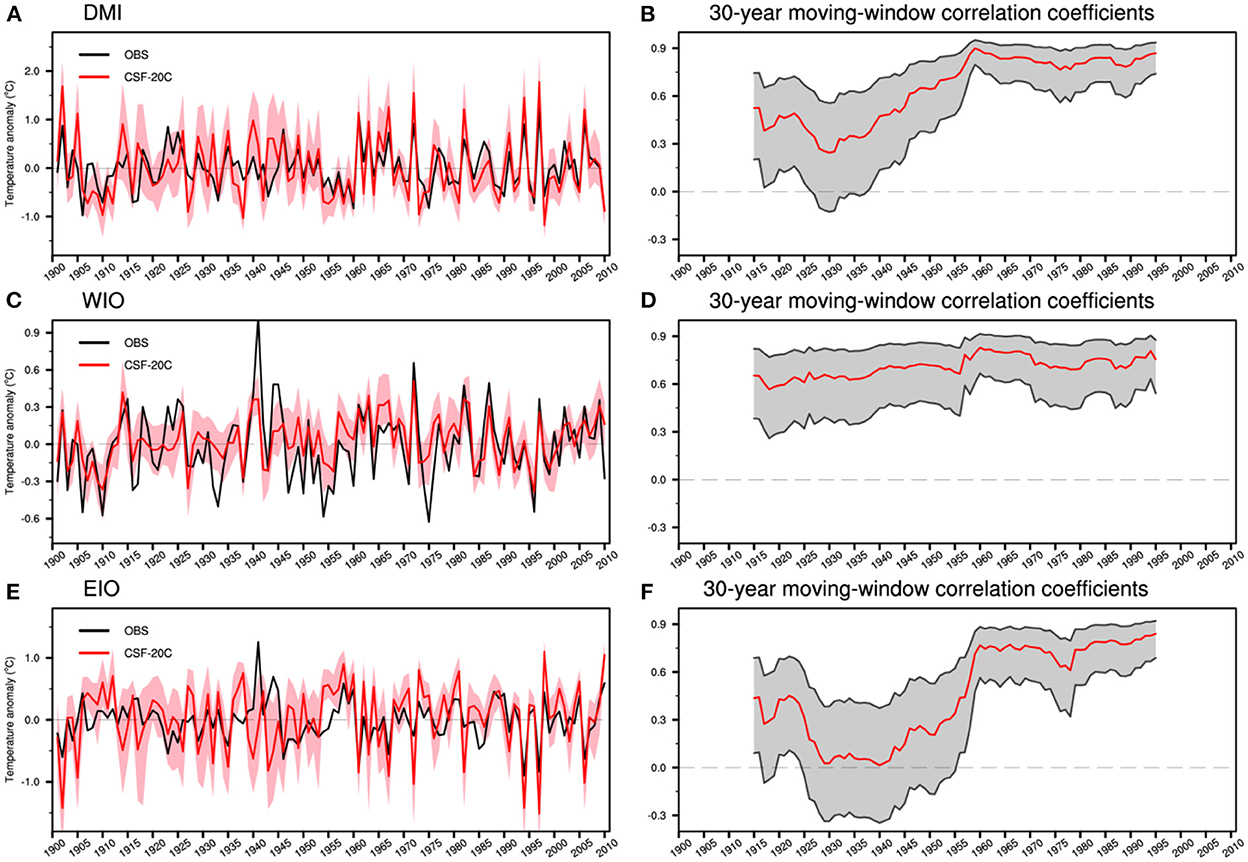
Figure 1. Left: (A) The SON-mean Indian Ocean dipole mode index (DMI) in observations (black line) and the 1-month lead ensemble mean predictions from the Coupled Seasonal Forecasts of the 20th century (CSF-20C) (red line). The red shading indicates the ensemble spread. (C, E) as in (A), but for predictions of the SON-mean western tropical Indian Ocean index (WIO) and the SON-mean tropical southeast Indian Ocean index (EIO). Right: the 30-year moving-window correlation coefficients between the ensemble mean prediction and the observations for (B) the SON-mean DMI, (D) the SON-mean WIO, and (F) the SON-mean EIO index. The correlation coefficients have been computed for 30-year windows moved across the period 1901–2010 by 1 year, and the correlations for each 30-year window are plotted at the central year. The gray-shaded bands in (B, D, F) indicate the 5–95% confidence intervals.
To demonstrate the decadal variations, the DMI correlation is calculated on a 30-year-long moving window (Figure 1B). The correlation skill shows significant decadal variations with a range of 0.24–0.90. The decadal variations of IOD prediction skill result from the decadal variation of prediction skill for the eastern pole of the IOD (Figures 1C–F). The prediction skill for the western pole of the IOD changes less during the whole 20th century (Figure 1D). For the eastern pole, the predictive skill is close to zero over the 1930–40s, rapidly grows over 1940–60s, and maintains at about 0.7 after 1960s (Figure 1F).
It is interesting to note that the decadal variation of IOD prediction skill is associated with the changes in predictive uncertainty, which can be measured by the ensemble member spread. The ensemble spreads of the predictions for the DMI, WIO, and EIO indices in the low-skill period are larger than those in the high-skill period (Figures 1A, C, E), indicating the changes in the strength of unpredictable noise.
To investigate the variations of the predictive skill for IOD, two typical periods, 1926–1955 (low-skill period) and 1981–2010 (high-skill period), are selected. It is conceivable that the difference in the IOD prediction skill between 1926–1955 and 1981–2010 may be associated with differences in the IOD events themselves. For the observation, the IOD events are similar in the tropical Indian Ocean and the tropical western Pacific in both stages (Figures 2, 3). In August, the negative SSTA off the coast of Sumatra-Java is coupled with the Sumatra-Philippine Sea teleconnection pattern, negative precipitation anomalies over the southeastern tropical Indian Ocean, positive precipitation anomalies over the western North Pacific and northward cross-equatorial wind anomalies (Li et al., 2006). From September to November, the IOD grows to the peak phase and then decays. The Sumatra-Philippine Sea teleconnection pattern gradually evolves to an anomalous anticyclone over the southeastern tropical Indian Ocean (Wang et al., 2003).
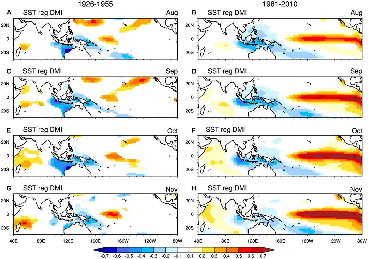
Figure 2. Regressions of monthly SSTA (unit: °C) onto the standardized SON-mean DMI index for the observation in the period 1926–1955: (A) August, (C) September, (E) October, and (G) November. Only values reaching the 5% significance level are shown. Right: (B, D, F, H) as in (A, C, E, G), but for the period 1981–2010.
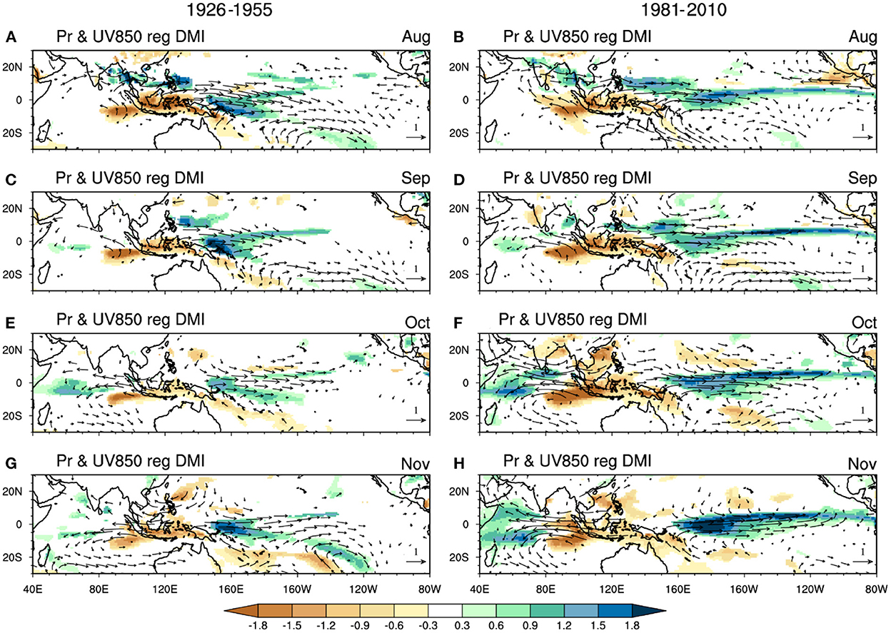
Figure 3. As in Figure 2, but for the regression of monthly precipitation (shading, unit: mm/day) and 850-hPa wind anomalies (vector, unit: m/s) for the period (A, C, E, G) 1926–1955, and (B, D, F, H) 1981–2010.
The main differences between the two stages are seen in the tropical Pacific. For the low-skill period of 1926–1955, the IOD events are less accompanied by ENSO, featured by statistically insignificant SSTA in the equatorial central-eastern Pacific associated with the IOD (Figure 2). The simultaneous correlation between the DMI and Niño-3.4 indices in 1926–1955 is only 0.23, not reaching even the 10% significance level. In contrast, for the high-skill period of 1981–2010, the IOD has close relationships with ENSO, with the simultaneous correlation between the DMI and Niño-3.4 indices reaching 0.70. The result indicates that the relationship between ENSO and IOD exhibits decadal variations in the observations.
Can the decadal variations of the ENSO-IOD relationship explain the decadal variations of IOD prediction skill? The correlation coefficients between the observed DMI and Niño-3.4 index calculated on a 30-year-long moving window are shown in Figures 4A, B. There are remarkable decadal variations of ENSO-IOD relationship in the observations, with their running correlations in a range of 0.10–0.77. Generally, the close (weak) ENSO-IOD relationship corresponds to high (low) IOD prediction skills. However, the variations of the ENSO-IOD relationship are not completely in pace with the decadal variations of IOD prediction skill (Figure 1B) (their correlation is 0.43), suggesting that there are other factors modulating the variations of the prediction skill.
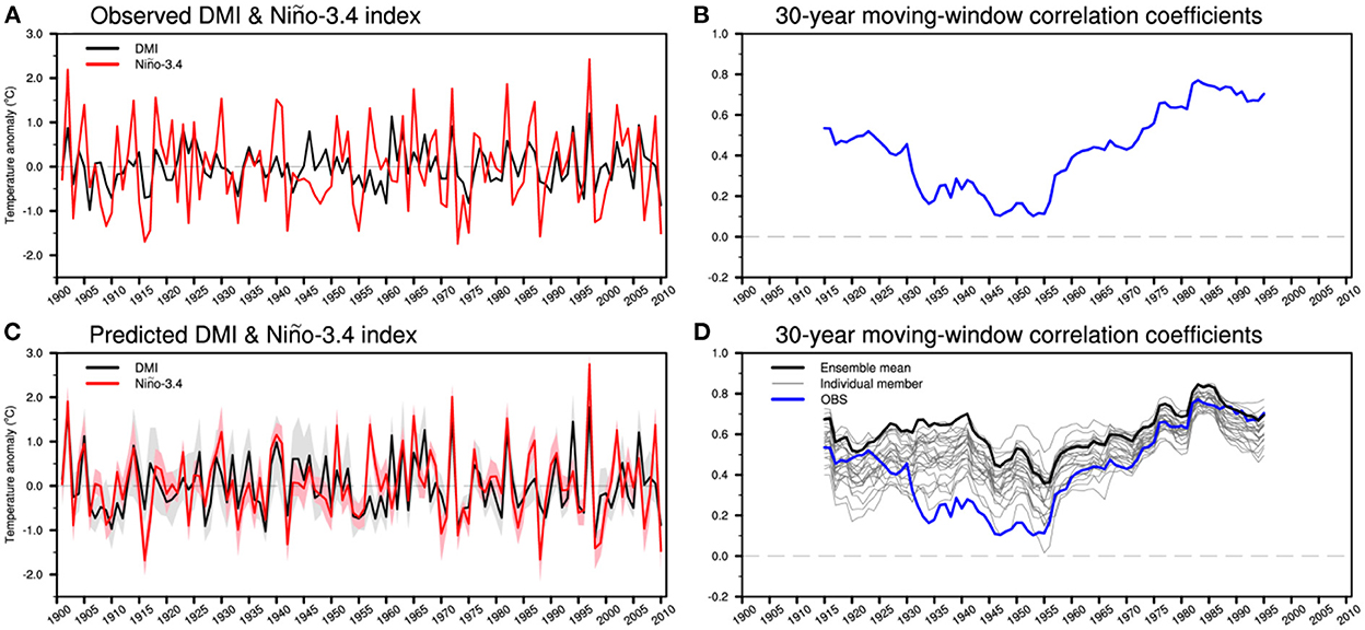
Figure 4. (A) The observed SON-mean DMI (black line) and SON-mean Niño-3.4 index (red line) for the period 1901–2010. (B) The 30-year moving-window correlation coefficients between the observed DMI and Niño-3.4 indices. (C) The predicted SON-mean DMI (black line) and SON-mean Niño-3.4 index (red line) at 1-month lead from the CSF-20C. The red and gray shading indicates the ensemble spread of DMI and Niño-3.4 index, respectively. (D) The 30-year moving-window correlation coefficients between the predicted DMI and Niño-3.4 indices for the ensemble mean (thick black line) and individual member (thin gray line). The observation is shown in a thick blue line. For (B, D), the correlation coefficients have been computed for 30-year windows moved across the period 1901–2010 by 1 year, and the correlations for each 30-year window are plotted at the central year.
We also check the decadal variations of the ENSO-IOD relationship in the predictions (Figure 4D). For individual members, the simulated ENSO-IOD relationships also have obvious decadal variations, with amplitudes being close to that in the observation for some cases. However, the decadal variations of the simulated ENSO-IOD relationship are not in phase among these members. As a result, after ensemble averaging is conducted, the decadal variation of the ENSO-IOD relationship is greatly suppressed. Meanwhile, the ENSO-IOD relationship becomes closer than any ensemble members. This means that simulated IOD events in the ensemble mean are persistently modulated by ENSO, different from IOD events in observation, which are sometimes out of the control of ENSO. As a result, the predictions would hit the target more easily for the period with IOD being also coupled with ENSO in the observation.
Both the observations and predictions contain predictable signals and unpredictable noises. Their relative magnitudes determine the SNR and the predictability. The ensemble members of predictions can generally cover the observed IOD variability (Figure 1A) and the observed ENSO-IOD relationship (Figures 4B, D), and thus we can approximatively see the observation as one of the ensemble prediction members. To understand the decadal variation of IOD prediction skill and predictability, we will investigate the formation processes of the predictable and unpredictable components in the model world in this section.
Under the assumption that the model is an approximate representation of the real world, we can extract the predictable component (signal) of IOD from the ensemble mean, and derive the unpredictable component (noise) from the deviations of individual prediction members from the ensemble mean (Hu et al., 2019). The strengths of the predictable signal and unpredictable noise of the DMI index calculated on a 30-year-long moving window are shown in Figure 5A. The decadal variation of the IOD signal strength matches well with the variation of prediction skill, with higher value in the early and second half of the 20th century (Figure 1B). The noise strength shows an inverse phase change with the signal strength and prediction skill. The changes in the strengths of IOD signal and noise result in the increase of the SNR in the second half of the 20th century (Figure 5B). The variations of the SNR are highly correlated with the decadal variations of IOD prediction skill (their correlation is 0.90, Figure 1B). This result indicates that the variations of predictive skill for IOD can be understood from the SNR analysis.
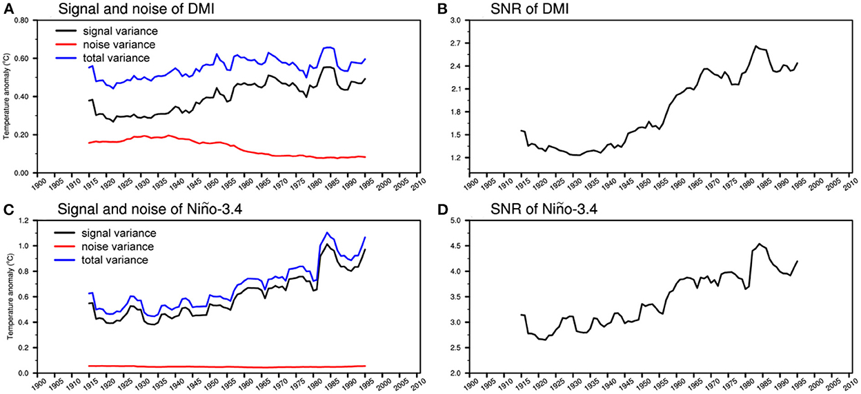
Figure 5. (A) The total variance (blue line), and the variance of predictable signal (black line) and unpredictable noise (red line) of the predicted SON-mean DMI. (B) The signal-to-noise ratio (SNR) of the predicted SON-mean DMI. The variance and SNR are calculated by the 30-year moving window for the period 1901–2010. (C, D) as in (A, B), but for the predicted SON-mean Niño-3.4 index.
What causes decadal variations of IOD SNR? As shown in Section Variations of the ENSO-IOD relationship, the predictable component (signal) of IOD derived from the ensemble mean is largely modulated by ENSO forcing. We first investigate the relationship in strength between the IOD signal and the ENSO signal based on the prediction system. The year-to-year variations of the predicted IOD index are closely linked with the predicted ENSO index in the ensemble mean prediction, with their correlation coefficient reaching 0.64 (Figure 4C), indicating that the decadal variations of the IOD signal strength are partly caused by the variations of ENSO signal strength.
To illustrate the influence of the ENSO signal on IOD prediction, Figure 6 shows the regression of the ensemble mean prediction of SSTA, precipitation, and 850-hPa circulation anomalies onto the IOD signal. Although IOD is de-coupled with ENSO variability in the 30-year low-skill period of 1926–1955 in observations, the predictable components closely parallel that of the high-skill period of 1981–2010. It can also be found that both the strengths of IOD and ENSO signal in the high-skill period are higher than that in the low-skill period, which is associated with the increase in the strength of ENSO signal since the 1930s (Figure 5C). For both periods, the ENSO-related warm SSTAs in the equatorial central-eastern Pacific stimulate alongshore wind anomalies off the Sumatra-Java coast in boreal summer via the anomalous Walker circulation, which further trigger the IOD through both the Bjerknes and “wind-evaporation-SST” feedbacks (Li et al., 2002; Yang et al., 2015).
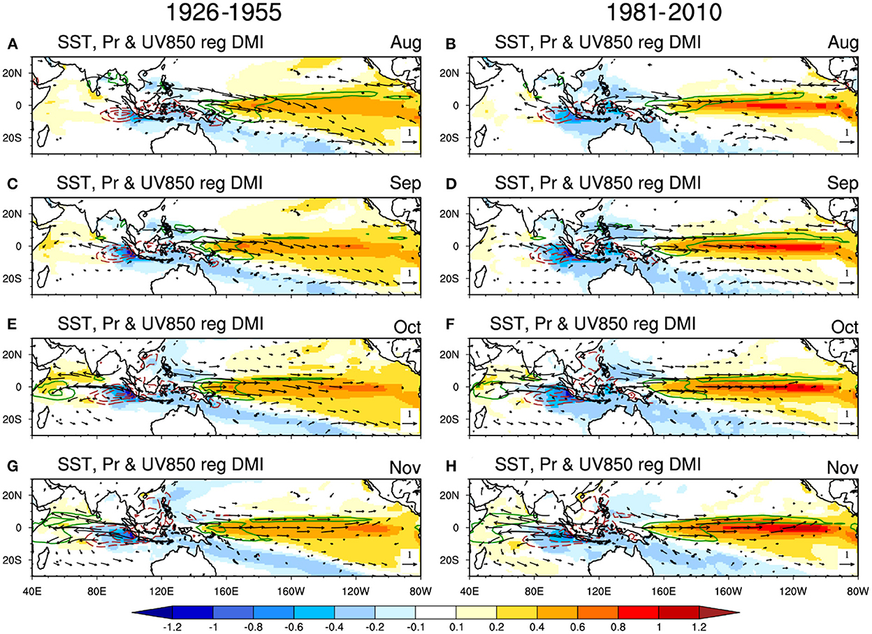
Figure 6. Left: Regression of monthly SSTA (shading, unit: °C), precipitation (contour, unit: mm/day), and 850-hPa wind anomalies (vector, unit: m/s) onto the standardized SON-mean DMI index from the ensemble mean predictions in the period 1926–1955: (A) August, (C) September, (E) October, and (G) November. Only values reaching the 5% significance level are shown. Right: (B, D, F, H) as in (A, C, E, G), but for the regression in the period 1981–2010.
The decadal variations of IOD SNR are also modulated by the strength of the IOD unpredictable component (noise). The most striking feature of the variations of IOD noise is that its strength gradually decreases during the second half of the 20th century (Figure 5A). The increase in the strength of the IOD signal and the decrease in the strength of IOD noise ultimately result in the increase of the SNR in the second half of the 20th century.
To illustrate the physical picture of the unpredictable component of IOD, we regress SST, precipitation and low-level wind anomalies from the ensemble spread onto the unpredictable component of DMI indices for the two typical periods (Figure 7). Both in the high-skill and low-skill periods, the unpredictable IODs exhibit similar evolution characteristics, with peaks in October and November. The unpredictable components are generally generated by the local air-sea interactions within the tropical Indian Ocean, with no significant correlation relationship with SSTA in other ocean basins. It is worth noting that the variations of the ENSO SNR are dominated by its variations of predictable signal strength, but independent of the noise strength (Figures 5C, D), consistent with previous studies (Tang et al., 2008; Hu et al., 2019). This is because the strength of the unpredictable components of ENSO keeps steady over the whole 20th century (Figure 5C). In contrast, the SNR of IOD is modulated by both the strengths of signal and noise as noted above. This suggests that the physical processes responsible for the predictability of IOD may be more complicated than that for ENSO, which involves both remote forcings from ENSO and internal air-sea interactions in the tropical Indian Ocean.
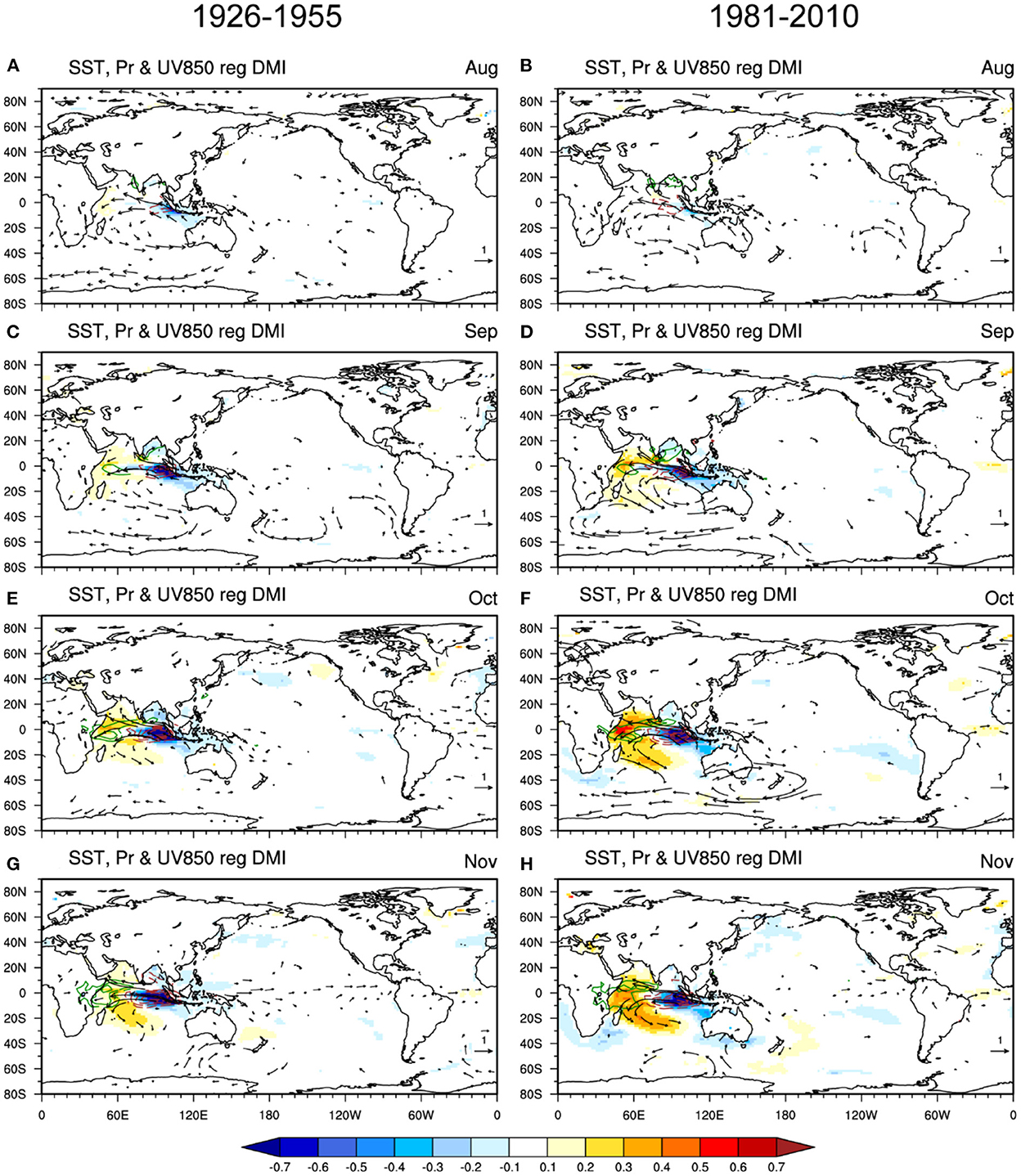
Figure 7. Left: Regression of monthly SSTA (shading, unit: °C), precipitation (contour, unit: mm/day), and 850-hPa wind anomalies (vector, unit: m/s) onto the standardized SON-mean DMI index from the ensemble spread in the period 1926–1955: (A) August, (C) September, (E) October, and (G) November. Only values reaching the 5% significance level are shown. Right: (B, D, F, H) as in (A, C, E, G), but for the regression in the period 1981–2010. For the regression analysis, all 25 members with the ensemble mean removed are connected to obtain a sample size as large as possible.
In this study, the decadal variations of IOD predictability are derived from the single model ensemble predictions, which may be model-dependent. We try to estimate the IOD predictability based on the persistence prediction using observational May-June-July mean SSTA (black line in Figure 8) (Wajsowicz, 2005). The correlation skill of the persistence prediction also shows decadal variations, though its amplitude is smaller than that of the correlation skill of the model dynamic prediction. This suggests that the decadal variations of IOD predictability during the past century are a robust characteristic.
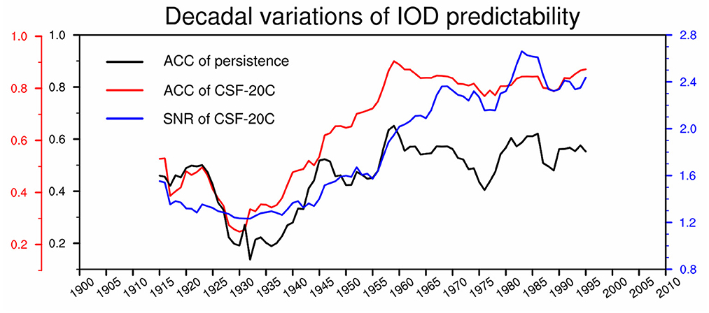
Figure 8. The 30-year moving-window ACC skill of SON-mean DMI for the CSF-20C predictions (red line) and the persistence predictions (black line). The signal-to-noise ratio (SNR) of the predicted SON-mean DMI calculated by the 30-year moving window for 1901−2010 is shown in the blue line. The persistence predictions of SON-mean DMI derived from the observational May-June-July mean SSTA.
In this study, we investigate the decadal variation of IOD prediction skills based on the century-scale seasonal hindcast experiments from the Coupled Seasonal Forecasts of the 20th century (CSF-20C). The major conclusions are summarized as follows.
First, for the predictions of boreal autumn IOD at the 1-month lead, the IOD prediction skill exhibits remarkable decadal variation, with low skill in the early-to-mid 20th century and high skill in the second half of the 20th century. The decadal variations of IOD prediction skill result from the decadal variation of prediction skill for the eastern pole of the IOD.
Second, the decadal variation of IOD prediction skill is influenced by the observed decadal variations of the ENSO-IOD relationship. There are remarkable decadal variations of the ENSO-IOD relationship in the observations. Although individual members of the predictions can simulate the variation of the ENSO-IOD relationship, with amplitude close to that in the observation, the feature is greatly suppressed in the ensemble mean due to the asynchrony of variation phases among individual members. In the ensemble mean, the IOD evolution shows an unrealistic stable and high correlation with ENSO evolution. This causes the prediction to have much higher skill for those periods during which IOD is accompanied by ENSO in the observation, and thus partly results in the decadal variations of IOD prediction skill.
Third, the decadal variation of IOD prediction skill is also modulated by the IOD predictability. In the prediction system, the decadal variation of IOD signal strength closely follows that of ENSO signal strength. Meanwhile, the IOD noise strength shows variations opposite to the IOD signal strength. As a result, the SNR and predictability of IOD greatly increase in the second half of the 20th century due to the enhancement of the ENSO signal strength, leading to variations of IOD prediction skills. The changes in the predictability of IOD in observation can be indirectly verified by the prediction skill of IOD persistence.
It is worth noting that the predictability measured by the SNR is estimated for the CSF-20C and thus is model-dependent. Similar long-term seasonal prediction experiments should be conducted by more models to check the robustness of conclusions obtained in the study.
In this study, we found that the IOD noise strength shows decadal variations inverse to the IOD signal strength. As a result, the total variance of IOD shows much weaker decadal variations (Figure 5A). We speculate that the strength of IOD variability is constrained by the intensities of local positive feedbacks responsible for the IOD growth, such as the wind-evaporation-SST feedback and the thermocline feedback. If the intensities of these feedbacks changed less, the total variance of IOD would remain unchanged, and the share of ENSO-forced and internal IOD would show an inverse change. This phenomenon deserves further study in the future, which may shed light on the projection of IOD intensity change under global warming. In addition, the warming rate in the tropical Indian Ocean is the fastest among all the tropical ocean basins (Roxy et al., 2014, 2020; Doi et al., 2020), The faster warming in the western tropical Indian Ocean than the eastern basin may modulate air-sea interactions over the tropical Indian Ocean and thus change IOD characteristics (Cai et al., 2013). How the zonally ununiform warming pattern in the Indian Ocean modulates IOD predictability deserves further study in the future.
As one of the most important variability modes at interannual timescales, the IOD has tremendous climate impacts. It is interesting to note that prediction skill for those regions modulated by IOD also shows decadal variations. Here, we take the boreal autumn precipitation anomalies over East Africa as an example. The land precipitation anomalies are closely linked to the IOD in both the observation and the simulations (Figures 9A, C). The prediction skill for the area-averaged precipitation anomalies over East Africa exhibits decadal variation similar to that of the prediction skill for the DMI indices (Figures 9B, D), with their correlation coefficient reaching 0.91, consistent with a recent study (Doi et al., 2022). This implies that it is essential to improve the prediction skill for dominant variability modes, which would improve the prediction skill for regional climates associated with these modes.
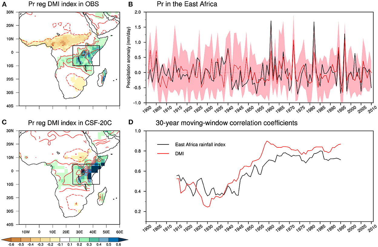
Figure 9. Left: the correlation coefficient between the SON-mean DMI index and SON-mean land precipitation [red contour, the positive (negative) values are shown in solid (dashed) lines; zero contour is not shown; interval is 0.2], and the regression of SON-mean land precipitation (shading, unit: mm/day) onto the SON-mean DMI index for (A) observation, (C) ensemble mean prediction. Right: (B) the SON-mean East Africa rainfall index (rainfall anomalies averaged over 10°S-5°N, 25°E-45°E) in observations (black line) and the ensemble mean predictions from the CSF-20C (red line). The red shading indicates the ensemble spread. (D) the 30-year moving-window correlation coefficients between the ensemble mean prediction and the observations for the SON-mean East Africa rainfall index (black line), and the SON-mean DMI (red line). The correlation coefficients have been computed for 30-year windows moved across the period 1901–2010 by 1 year, and the correlations for each 30-year window are plotted at the central year.
The original contributions presented in the study are included in the article/supplementary material, further inquiries can be directed to the corresponding author.
BW designed the research, provided comments, and revised the manuscript. SH performed the analysis and drafted the manuscript. TZ revised the manuscript. All authors contributed to the article and approved the submitted version.
This work was jointly supported by the National Natural Science Foundation of China (Grants 42075163 and 42205039) and the China Postdoctoral Science Foundation under Grant 2022T150638.
The authors declare that the research was conducted in the absence of any commercial or financial relationships that could be construed as a potential conflict of interest.
All claims expressed in this article are solely those of the authors and do not necessarily represent those of their affiliated organizations, or those of the publisher, the editors and the reviewers. Any product that may be evaluated in this article, or claim that may be made by its manufacturer, is not guaranteed or endorsed by the publisher.
Annamalai, H., Xie, S. P., McCreary, J. P., and Murtugudde, R. (2005). Impact of Indian Ocean Sea surface temperature on developing El Niño*. J. Clim. 18, 302–319. doi: 10.1175/JCLI-3268.1
Ashok, K., Guan, Z., and Yamagata, T. (2001). Impact of the Indian Ocean dipole on the relationship between the Indian monsoon rainfall and ENSO. Geophys. Res. Lett. 28, 4499–4502. doi: 10.1029/2001GL013294
Baquero-Bernal, A., Latif, M., and Legutke, S. (2002). On dipolelike variability of sea surface temperature in the Tropical Indian Ocean. J. Clim. 15, 1358–1368. doi: 10.1175/1520-0442(2002)015
Barnston, A. G., Tippett, M. K., Ranganathan, M., and L'Heureux, M. L. (2019). Deterministic skill of ENSO predictions from the North American Multimodel Ensemble. Clim. Dyn. 53, 7215–7234. doi: 10.1007/s00382-017-3603-3
Behera, S. K., Luo, J. J., Masson, S., Rao, S. A., Sakuma, H., Yamagata, T., et al. (2006). A CGCM study on the interaction between IOD and ENSO. J. Clim. 19, 1688–1705. doi: 10.1175/JCLI3797.1
Black, E. (2005). The relationship between Indian Ocean sea-surface temperature and East African rainfall. Philos. Trans. A Math. Phys. Eng. Sci. 363, 43–47. doi: 10.1098/rsta.2004.1474
Cai, W., and Cowan, T. (2013). Why is the amplitude of the Indian Ocean Dipole overly large in CMIP3 and CMIP5 climate models? Geophys. Res. Lett. 40, 1200–1205. doi: 10.1002/grl.50208
Cai, W., van Rensch, P., Cowan, T., and Hendon, H. H. (2011). Teleconnection pathways of ENSO and the IOD and the mechanisms for impacts on Australian rainfall. J. Clim. 24, 3910–3923. doi: 10.1175/2011JCLI4129.1
Cai, W., Zheng, X-T., Weller, E., Collins, M., Cowan, T., et al. (2013). Projected response of the Indian Ocean Dipole to greenhouse warming. Nat. Geosci. 6, 999–1007. doi: 10.1038/ngeo2009
Chen, D., Cane, M. A., Kaplan, A., Zebiak, S. E., and Huang, D. (2004). Predictability of El Nino over the past 148 years. Nature. 428, 733–736. doi: 10.1038/nature02439
Doi, T., Behera, S. K., and Yamagata, T. (2020). Wintertime impacts of the 2019 Super IOD on East Asia. Geophys. Res. Lett. 47, e2020GL089456. doi: 10.1029/2020GL089456
Doi, T., Behera, S. K., and Yamagata, T. (2022). On the predictability of the extreme drought in East Africa during the short rains season. Geophys. Res. Lett. 49, e2022GL100905. doi: 10.1029/2022GL100905
Doi, T., Storto, A., Behera, S. K., Navarra, A., and Yamagata, T. (2017). Improved prediction of the Indian Ocean dipole mode by use of subsurface ocean observations. J. Clim. 30, 7953–7970. doi: 10.1175/JCLI-D-16-0915.1
Goddard, L., Kumar, A., Solomon, A., Smith, D., Boer, G., Gonzalez, P., et al. (2013). A verification framework for interannual-to-decadal predictions experiments. Clim. Dyn. 40, 245–272. doi: 10.1007/s00382-012-1481-2
Guan, Z., and Yamagata, T. (2003). The unusual summer of 1994 in East Asia: IOD teleconnections. Geophys. Res. Lett. 30, 1544. doi: 10.1029/2002GL016831
Horii, T., Hase, H., Ueki, I., and Masumoto, Y. (2008). Oceanic precondition and evolution of the 2006 Indian Ocean dipole. Geophys. Res. Lett. 35, L03607. doi: 10.1029/2007GL032464
Hu, Z-Z., Kumar, A., Zhu, J., Peng, P., and Huang, B. (2019). On the challenge for ENSO cycle prediction: an example from NCEP climate forecast system, Version 2. J. Clim. 32, 183–194. doi: 10.1175/JCLI-D-18-0285.1
Huang, B., Thorne, P. W., Banzon, V. F., Boyer, T., Chepurin, G., Lawrimore, J. H., et al. (2017). Extended reconstructed sea surface temperature, version 5 (ERSSTv5): Upgrades, validations, and intercomparisons. J. Clim. 30, 8179–8205. doi: 10.1175/jcli-d-16-0836.1
Izumo, T., Vialard, J., Lengaigne, M., Boyer Montegut, C. de., Behera, S. K., Luo, J.-J., et al. (2010). Influence of the state of the Indian Ocean dipole on the following year's El Niño. Nat. Geosci. 3, 168–172. doi: 10.1038/ngeo760
Kirtman, B. P., Min, D., Infanti, J. M., Kinter, J. L., Paolino, D. A., Zhang, Q., et al. (2014). The North American multimodel ensemble: phase-1 seasonal-to-interannual prediction; phase-2 toward developing intraseasonal prediction. Bull. Am. Meteorol. Soc. 95, 585–601. doi: 10.1175/BAMS-D-12-00050.1
Kirtman, B. P., and Schopf, P. S. (1998). Decadal variability in ENSO predictability and prediction. J. Clim. 11, 2804–2822.
Laloyaux, P., Boisseson, E., de Balmaseda, M., Bidlot, J-R., Broennimann, S., Buizza, R., et al. (2018). CERA-20C: a coupled reanalysis of the twentieth century. J. Adv. Model. Earth Syst. 10, 1172–1195. doi: 10.1029/2018MS001273
Li, T., Liu, P., Fu, X., Wang, B., and Meehl, G. A. (2006). Spatiotemporal structures and mechanisms of the tropospheric biennial oscillation in the Indo-Pacific Warm Ocean Regions*. J. Clim. 19, 3070–3087. doi: 10.1175/JCLI3736.1
Li, T., Wang, B., Chang, C. P., and Zhang, Y. (2003). A theory for the Indian Ocean dipole–zonal mode*. J. Atmos. Sci. 60, 2119–2135. doi: 10.1175/1520-0469(2003)060<2119:Atftio>2.0.Co;2
Li, T., Zhang, Y., Lu, E., and Wang, D. (2002). Relative role of dynamic and thermodynamic processes in the development of the Indian Ocean dipole: an OGCM diagnosis. Geophys. Res. Lett. 29, 25–21-25-24. doi: 10.1029/2002GL015789
Liu, H., Tang, Y., Chen, D., and Lian, T. (2016). Predictability of the Indian Ocean Dipole in the coupled models. Clim. Dyn. 48, 2005–2024. doi: 10.1007/s00382-016-3187-3
Liu, T., Song, X., Tang, Y., Shen, Z., and Tan, X. (2022). ENSO predictability over the Past 137 years based on a CESM ensemble prediction system. J. Clim. 35, 763–777. doi: 10.1175/JCLI-D-21-0450.1
Lu, B., and Ren, H. L. (2020). What caused the extreme Indian Ocean dipole event in 2019? Geophys. Res. Lett. 47, e2020GL087768. doi: 10.1029/2020GL087768
Lu, Z., Dong, W., Lu, B., Yuan, N., Ma, Z., Bogachev, M. I., et al. (2022). Early warning of the Indian Ocean Dipole using climate network analysis. Proc. Natl. Acad. Sci. USA. 119, e2109089119. doi: 10.1073/pnas.2109089119
Luo, J-.J., Masson, S., Behera, S., and Yamagata, T. (2007). Experimental forecasts of the Indian Ocean dipole using a coupled OAGCM. J. Clim. 20, 2178–2190. doi: 10.1175/JCLI4132.1
Luo, J-J., Behera, S., Masumoto, Y., Sakuma, H., and Yamagata, T. (2008). Successful prediction of the consecutive IOD in 2006 and 2007. Geophys. Res. Lett. 35, L14S02. doi: 10.1029/2007GL032793
Luo, J-J., Zhang, R., Behera, S. K., Masumoto, Y., Jin, F-, F., Lukas, R., et al. (2010). Interaction between El Niño and extreme Indian Ocean dipole. J. Clim. 23, 726–742. doi: 10.1175/2009JCLI3104.1
Nuncio, M., and Yuan, X. (2015). The influence of the Indian Ocean dipole on Antarctic Sea Ice*. J. Clim. 28, 2682–2690. doi: 10.1175/JCLI-D-14-00390.1
Qiu, Y., Cai, W., Guo, X., and Ng, B. (2014). The asymmetric influence of the positive and negative IOD events on China's rainfall. Sci. Rep. 4, 4943. doi: 10.1038/srep04943
Roxy, M. K., Gnanaseelan, C., Parekh, A., Chowdary, J. S., Singh, S., Modi, A., et al. (2020). Indian Ocean warming. Assessment of Climate Change over the Indian Region, 191–206. doi: 10.1007/978-981-15-4327-2_10
Roxy, M. K., Ritika, K., Terray, P., and Masson, S. (2014). The curious case of Indian Ocean warming*,+. J. Clim. 27, 8501–8509. doi: 10.1175/JCLI-D-14-00471.1
Saji, N. H., Goswami, B. N., Vinayachandran, P. N., and Yamagata, T. (1999). A dipole mode in the tropical Indian Ocean. Nature. 401, 360–363. doi: 10.1038/43854
Shi, L., Hendon, H. H., Alves, O., Luo, J. J., Balmaseda, M., Anderson, D., et al. (2012). How predictable is the Indian Ocean dipole? Mon. Weather Rev. 140, 3867–3884. doi: 10.1175/MWR-D-12-00001.1
Song, X., Tang, Y., and Chen, D. (2018). Decadal variation in IOD predictability during 1881-2016. Geophys. Res. Lett. 45, 12948–12956. doi: 10.1029/2018GL080221
Song, X., Tang, Y., Liu, T., and Li, X. (2022). Predictability of Indian Ocean dipole over 138 years using a CESM ensemble-prediction system. J. Geophys. Res. Oceans. 127, e2021JC018210. doi: 10.1029/2021JC018210
Stuecker, M. F., Timmermann, A., Jin, F-F., Chikamoto, Y., Zhang, W., Wittenberg, A. T., et al. (2017). Revisiting ENSO/Indian Ocean Dipole phase relationships. Geophysical Research Letters. 44, 2481–2492. doi: 10.1002/2016GL072308
Sun, S., Lan, J., Fang, Y., and Tana Gao, X. (2015). A triggering mechanism for the Indian Ocean dipoles independent of ENSO. J. Clim. 28, 5063–5076. doi: 10.1175/JCLI-D-14-00580.1
Tang, Y., Deng, Z., Zhou, X., Cheng, Y., and Chen, D. (2008). Interdecadal variation of ENSO predictability in multiple models. J. Clim. 21, 4811–4833. doi: 10.1175/2008JCLI2193.1
Tang, Y., Zhang, R-H., Liu, T., Duan, W., Yang, D., Zheng, F., et al. (2018). Progress in ENSO prediction and predictability study. Natl. Sci. Rev. 5, 826–839. doi: 10.1093/nsr/nwy105
Tompkins, A. M., Ortiz De Zárate, M. I., Saurral, R. I., Vera, C., Saulo, C., Merryfield, W. J., et al. (2017). The climate-system historical forecast project: providing open access to seasonal forecast ensembles from centers around the globe. Bull. Am. Meteorol. Soc. 98, 2293–2301. doi: 10.1175/BAMS-D-16-0209.1
Tozuka, T., Luo, J-J., Masson, S., and Yamagata, T. (2007). Decadal modulations of the Indian Ocean dipole in the SINTEX-F1 coupled GCM. J. Clim. 20, 2881–2894. doi: 10.1175/JCLI4168.1
Ummenhofer, C. C., England, M. H., McIntosh, P. C., Meyers, G. A., Pook, M. J., Risbey, J. S., et al. (2009). What causes southeast Australia's worst droughts? Geophys. Res. Lett. 36, L04706. doi: 10.1029/2008GL036801
Wajsowicz, R. C. (2005). Potential predictability of tropical Indian Ocean SST anomalies. Geophys. Res. Lett. 32, L24702. doi: 10.1029/2005GL024169
Wang, B., Lee, J-Y., Kang, I-S., Shukla, J., Park, C. K., et al. (2008). Advance and prospectus of seasonal prediction: assessment of the APCC/CliPAS 14-model ensemble retrospective seasonal prediction (1980–2004). Clim. Dyn. 33, 93–117. doi: 10.1007/s00382-008-0460-0
Wang, B., Wu, R., and Li, T. (2003). Atmosphere–warm ocean interaction and its impacts on asian–australian monsoon variation*. J. Clim. 16, 1195–1211. doi: 10.1175/1520-0442(2003)16<1195:Aoiaii>2.0.Co;2
Webster, P. J., Moore, A. M., Loschnigg, J. P., and Leben, R. R. (1999). Coupled ocean-atmosphere dynamics in the Indian Ocean during 1997-98. Nature. 401, 356–360. doi: 10.1038/43848
Weisheimer, A., Balmaseda, M. A., Stockdale, T. N., Mayer, M., Sharmila, S., Hendon, H., et al. (2022). Variability of ENSO forecast skill in 2-year global reforecasts over the 20th century. Geophys. Res. Lett. 49, e2022GL097885. doi: 10.1029/2022GL097885
Weisheimer, A., Befort, D. J., MacLeod, D., Palmer, T., O'Reilly, C., Strømmen, K., et al. (2020). Seasonal forecasts of the 20th Century. Bulletin of the American Meteorological Society. 101, 8. doi: 10.1175/BAMS-D-19-0019.1
Yang, Y., Xie, S-P., Wu, L., Kosaka, Y., Lau, N-C., and Vecchi, G. A. (2015). Seasonality and predictability of the Indian Ocean dipole mode: ENSO forcing and internal variability. J. Clim. 28, 8021–8036. doi: 10.1175/JCLI-D-15-0078.1
Yu, J-Y., and Lau, K. M. (2004). Contrasting Indian Ocean SST variability with and without ENSO influence: a coupled atmosphere-ocean GCM study. Meteorol. Atmospheric Phys. 90, 179–191. doi: 10.1007/s00703-004-0094-7
Zhang, L. Y., Du, Y., Cai, W., Chen, Z., Tozuka, T., Yu, J. Y., et al. (2020). Triggering the Indian Ocean dipole from the southern hemisphere. Geophys. Res. Lett. 47, e2020GL088648. doi: 10.1029/2020GL088648
Zhang, Y., Li, J., Xue, J., Feng, J., Wang, Q., Xu, Y., et al. (2018). Impact of the South China sea summer monsoon on the Indian Ocean Dipole. J. Clim. 31, 6557–6573. doi: 10.1175/JCLI-D-17-0815.1
Zhang, Y., Li, J., Xue, J., Zheng, F., Wu, R., Ha, K-J, et al. (2019). The relative roles of the South China Sea summer monsoon and ENSO in the Indian Ocean dipole development. Clim. Dyn. 53, 6665–6680. doi: 10.1007/s00382-019-04953-4
Zhao, S., Jin, F. F., and Stuecker, M. F. (2019). Improved predictability of the Indian Ocean dipole using seasonally modulated ENSO forcing forecasts. Geophys. Res. Lett. 46, 9980–9990. doi: 10.1029/2019GL084196
Keywords: Indian Ocean dipole mode, seasonal prediction, predictability, signal-to-noise ratio (S/N ratio), El Niño–Southern Oscillation (ENSO)
Citation: Hu S, Wu B and Zhou T (2023) Decadal variation of prediction skill for Indian Ocean dipole over the past century. Front. Clim. 4:1082026. doi: 10.3389/fclim.2022.1082026
Received: 27 October 2022; Accepted: 14 December 2022;
Published: 06 January 2023.
Edited by:
Matthew Collins, University of Exeter, United KingdomReviewed by:
F. Feba, University of Hyderabad, IndiaCopyright © 2023 Hu, Wu and Zhou. This is an open-access article distributed under the terms of the Creative Commons Attribution License (CC BY). The use, distribution or reproduction in other forums is permitted, provided the original author(s) and the copyright owner(s) are credited and that the original publication in this journal is cited, in accordance with accepted academic practice. No use, distribution or reproduction is permitted which does not comply with these terms.
*Correspondence: Bo Wu,  d3Vib0BtYWlsLmlhcC5hYy5jbg==
Disclaimer: All claims expressed in this article are solely those of the authors and do not necessarily represent those of their affiliated organizations, or those of the publisher, the editors and the reviewers. Any product that may be evaluated in this article or claim that may be made by its manufacturer is not guaranteed or endorsed by the publisher.
Research integrity at Frontiers
Learn more about the work of our research integrity team to safeguard the quality of each article we publish.