A modified deep learning weather prediction using cubed sphere for global precipitation

Deep learning (DL), a potent technology to develop Digital Twin (DT), for weather prediction using cubed spheres (DLWP-CS) was recently proposed to facilitate data-driven simulations of global weather fields. DLWP-CS is a temporal mapping algorithm wherein time-stepping is performed through U-NET. Although DLWP-CS has shown impressive results for fields, such as temperature and geopotential height, this technique is complicated and computationally challenging for a complex, non-linear field, such as precipitation, which depends on other prognostic environmental co-variables. To address this challenge, we modify the DLWP-CS and call our technique “modified DLWP-CS” (MDLWP-CS). In this study, we transform the architecture from a temporal to a spatio-temporal mapping (multivariate setup), wherein precursor(s) of precipitation can be used as input. As a proof of concept, as a first simple case, a 2-m surface air temperature is used to predict precipitation using MDLWP-CS. The model is trained using hourly ERA-5 reanalysis and the resulting experimental findings are compared to two benchmark models, viz, the linear regression and an operational numerical weather prediction model, which is the Global Forecast System (GFS). The fidelity of MDLWP-CS is much better compared to linear regression and the results are equivalent to GFS output in terms of daily precipitation prediction with 1 day lag. These results provide an encouraging framework for an efficient DT that can facilitate speedy, high fidelity precipitation predictions.

1. Introduction

Precipitation prediction is important for many applications at different scales for socio-economic decision-making. Numerical weather prediction (NWP) models are one of the best tools for such predictions. However, reliable precipitation prediction at a higher resolution is still a challenge for the NWP models (Dimri and Niyogi, 2013; Kidd et al., 2013; Rao et al., 2019; Lavers et al., 2021). Representing an accurate relationship of precipitation to prognostic variables within the NWP systems contributes to the accuracy of forecasted rainfall (Maher et al., 2018). In addition to the challenges in the representation of physical processes, there are several uncertainties existing in the present-day NWP system (Yano et al., 2018). Thus, simpler, computationally efficient, and more cost-effective approaches are needed for predicting precipitation.

In the last decade, deep learning (DL), a potent technology to develop Digital Twin (DT), has emerged as a framework to solve complex, nonlinear problems by unwrapping the non-linearity in different layers of a deep neural network (Zeiler and Fergus, 2014). The developments, particularly in the field of computer vision, have led to efficient solutions to problems such as recognizing handwritten and other decodings, which were not possible a decade back. These advances have come about due to different factors such as the availability of hardware capable of performing memory-intensive convolution operations, which were not available when convolution neural networks (CNN) were first proposed (LeCun et al., 1998). Moreover, software stack development, such as open-source python libraries (TensorFlow, PyTorch, Theano, and others), has contributed to lowering the entry barriers for DL. The advancement in DL methods has gained prominence in the computer vision and other communities fomenting interest to build a DT framework for weather prediction. Moreover, DL-based weather prediction can yield output at a fraction of the computational cost relative to the traditional NWPs.

Recently, various efforts have focused on the weather prediction of global data fields, such as geopotential height, wind, and temperature (prognostic variables), using DL as an alternative to NWP (Rasp and Lerch, 2018; Scher, 2018; Scher and Messori, 2019; Arcomano et al., 2020; Han et al., 2020; Sønderby et al., 2020; Yuval and O'Gorman, 2020; Bihlo, 2021; Espeholt et al., 2021; Ravuri et al., 2021; Yuval et al., 2021; Bihlo and Popovych, 2022). However, there have been limited attempts toward forecasting the global precipitation (diagnostic variables), which is the most challenging variable to predict (Scher, 2018; Scher and Messori, 2019; Arcomano et al., 2020; Bihlo, 2021). Moreover, the literature described earlier lacks comparison with the operational products and the representation of the spherical structure of the global datasets.

Initial studies by Weyn et al. (2019) and Weyn et al. (2020) attempted to resolve the issue of addressing global data sphericity that had not been considered in the previous literature. According to Weyn et al. (2019), U-NET was applied to predict the 500-hPa geopotential height using the reanalysis dataset (Deep Learning Weather Prediction, DLWP). In a follow-up study, Weyn et al. (2020) introduced the cubed sphere to transform the spherical global data while using U-NET (Deep Learning Weather Prediction-cubed spheres, DLWP-CS) to predict the 500-hPa geopotential height and 850-hPa temperature. Both methods (DLWP and DLWP-CS) perform a temporal learning framework similar to the traditional autoregressive integrated moving average model (ARIMA) or recurrent neural network (RNN) (predict geopotential height at t+1 time steps using inputs from time t) models to demonstrate that U-NET can be used for NWP prediction. In other words, the same variables need to be present in the input and output for the model implementation. In that way, they intend to develop a self-sustaining model independent of the existing NWPs. The output can be recursively fed as the input, and a simulation similar to NWPs can be performed. The minimization of spherical distortion by the six-faced cubed sphere projection (cubed sphere mapping), which was taken as images, helped reduce the model biases. This was a choice aimed to benefit from the developments in the field of DL and computer vision. The global spherical dataset involves transformations into the cubed sphere projection. Although DLWP-CS has shown impressive results for fields, such as geopotential height and temperature, it would be more complicated and computationally challenging for a complex, non-linear field, such as precipitation, where auto-correlation is poor and is dependent on many other prognostic environmental co-variables (precursors). Briefly, DLWP and DLWP-CS work using a temporal mapping algorithm, wherein time-stepping is performed by the U-NET. However, this method is challenging for multivariate setup due to computational requirements where variables of interest are dependent on various predictors.

To address the challenges discussed earlier, we modify the DLWP-CS and call our technique “modified DLWP-CS” (MDLWP-CS) to transform the U-NET architecture from a temporal transformation (univariate) to a spatio-temporal mapping (multi-variate), wherein precursor(s) of precipitation can be used as an input. This modification, we hypothesize, would allow the capture of the linkages from physically relevant simple precursors to predict precipitation while maintaining the dynamical scale teleconnections. A schematic of the MDLWP-CS is presented in Figure 1. Our work serves as a continuation of a methodology for fast and reliable global precipitation predictions as part of a DT.

FIGURE 1

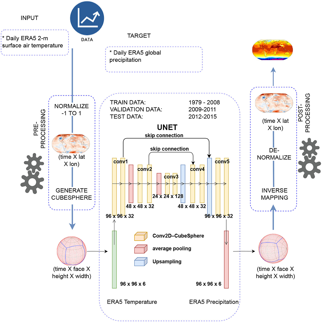
Figure 1. Schematic showing the U-NET modified DLWP-CS (Cubed Sphere)-based deep learning algorithm for learning Earth system physics toward fast and reliable precipitation forecasts.

The rest of the paper is organized as follows: The dataset used in the study is described in Section 2. Methodology and implementation strategy are described in Sections 3, 4, respectively. Section 5 outlines the results and discussion The study conclusions are outlined in Section 6 along with the discussion about future scope.

2. Datasets

2.1. Reanalysis dataset

Our proposed MDLWP-CS model is trained using hourly data from ERA-5 reanalysis download from the Weatherbench (https://github.com/pangeo-data/WeatherBench). Weatherbench provides a baseline dataset derived from the ERA5 archive that has been processed to facilitate its use in ML models. This database comprises 15 variables and is available in three spatial resolutions (1.4, 2.8, and 5.6 degrees). The details of this database can be found in Rasp et al. (2020). Owing to the physical linkages to precipitation and the computational and disk-storage constraints and the objective of creating simple and efficient DT, we use only 2-m surface air temperature as input and precipitation as the DL model's output. The dataset with 1.4° spatial resolution from 1979 to 2015 is used for this study. We used the time periods from 1979 to 2009 for model training, 2010–2011 for model validation, and 2012–2015 for model testing.

2.2. Dataset from global forecast system

We used the day-1 lead precipitation forecasts from GFS during 2012–2015 to compare MDLWP-CS output with the operational numerical weather prediction model. It is a T574 global spectral model forced with fixed oceanic conditions. The output corresponding to the years 2012–2015 is used for precipitation, which is available globally at daily temporal scales. The model is operationally run at IITM Pune on NVIDIA Tesla P100 GPU in the Cray XC50 machine (Prasad et al., 2011).

3. Methodology

In this section, the concept of DLWP and DLWP-CS as well as the proposed MDLWP-CS is described. The benchmark models used for comparison are also discussed.

3.1. Familiarization with DLWP and DLWP-CS

A deep convolutional neural network (CNN) with a U-shaped architecture (U-NET) is at the heart of the DLWP model (Weyn et al., 2019). The goal of a DLWP model is to take the multidimensional atmospheric state u(t) at a particular time and return the condition of the atmosphere at some future period, u(t+Δt). By using past weather as training data, DLWP directly translates the present state u(t) to the expected future state u(t+ Δt) predicting geopotential height. This method is similar to the RNN or ARIMA where it performs temporal learning. This method was further improved by transforming the spherical global data into the CS mapping while using U-NET (DLWP-CS) (Weyn et al., 2020). The CS remapping minimizes the distortion on the cube faces on which convolution operations are performed and provides natural boundary conditions for padding in the CNN, which produces weather forecasts that are stable and produce realistic weather patterns (Weyn et al., 2020). CS is inherently a spherical cube with six faces, four along the tropics and two representing the poles. The latitude–longitude data are represented on the CS to ensure that the errors arising due to sphericity of global data are minimized. Various mathematical operations such as convolution, nonlinear activation, and max-pooling are applied to the images or faces of the CS. In DLWP-CS, the same variables need to be present in the input and output for the model implementation in a way to develop an independent self-sustaining model similar to NWP. In other ways, the output of DLWP-CS can be recursively fed as an input within the system and a simulation similar to NWP can be performed. Weyn et al. (2020) compared their results from DLPW-CS with the Integrated Forecasting System (IFS42) at the European Centre for Medium-Range Weather Forecasting (ECMWF) and found that the DLWP-CS outperformed IFS42.

3.2. Overview of the proposed MDLWP-CS

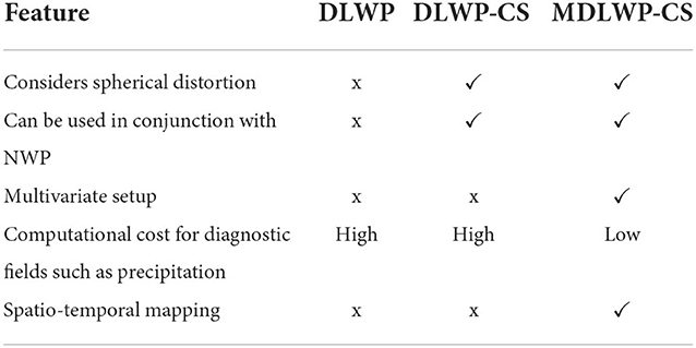
As discussed in Section 1, both DLWP and DLWP-CS are limited to a multivariate setup where the variables of interest, such as precipitation, are dependent on many other prognostic environmental co-variables (precursors). With DLWP and DLWP-CS models, the computational cost for predicting precipitation would be very high due to the multivariate nature of the problem. Table 1 discusses the major differences between DLWP, DLWP-CS, and the proposed MDLWP-CS. The number of inputs and targets in MDLWP-CS can be variable, whereas DLWP and DLWP-CS need an equal number of variables as inputs and targets. Once the model is trained, the time for the forecast (generate output) is much faster in MDLWP-CS. This is a notable advantage of using a DL-based system relative to the NWP system to reduce the computational cost for real-time prediction.

TABLE 1

Table 1. Comparison of DLWP, DLWP-CS, and the proposed MDLWP-CS.

3.3. Benchmark models

The performance of MDLWP-CS is compared to two benchmark models, viz, the linear regression and an operational numerical weather prediction model, the Global Forecast System (GFS) (Prasad et al., 2011). The comparison is done on the day-1 lead forecast output from GFS, linear regression, and the DL-based global model output.

Linear regression models are developed at each grid point on Earth with the surface air temperature as the independent variable and precipitation as the dependent target. The linear regression model uses the same hourly ERA-5 reanalysis data for training as MDLWP-CS. The hourly data are aggregated at a daily time-scale and are used for comparison with MDLWP-CS. The period 1979–2011 is used for training and 2012–2015 is used for testing.

4. Implementation

To test our proposed MDLWP-CS, as a first simple case, and also owing to the physical linkages of temperature to precipitation and the computational as well as disk-storage constraints, a 2-m surface air temperature is used to predict precipitation using MDLWP-CS. The MDLWP-CS uses features such as early stopping, a custom CubedSphereConv2D class to map one variable to another, and a custom data generator to facilitate training, validation, and testing. In this section, the implementation strategy of MDLWP-CS is described.

4.1. Data preprocessing and required computational platform

All the fields (2-m surface air temperature as input and precipitation as target) are first normalized using min–max scaling and preprocessed to a CS mapping, which is then used to train the model. When the spherical dataset is transformed into CS, we need to select the spatial resolution of the six CS faces to reduce spherical distortion. We did forward and reverse mapping to choose the CS resolution, which minimized the transformation error. We found that for our 1,024 × 1,024 spatial resolution (1.4°) would be ideal; however, with the available hardware (Intel(R) Xeon(R) CPU E5-2695 v4 @ 2.10GHz) used for the CS mapping, it was possible to only transform one-time step (1 h) at a time to 1024x1024. The GPU used for this work is NVIDIA Tesla P100 (12 GB GPU RAM) on the Cray XC50. Hence, we chose 512x512 as the CS resolution to transform 24-time steps (i.e., 1 day) to CS in a single step. However, after the U-NET model was created, it was found that the NVIDIA Tesla P100 (12 GB) GPU only supported a single batch and single channel as the input and output, that is, (1, 6, 512, 512, 1) to (1, 6, 512, 512, 1), where the indices correspond to batches, faces, height, width, and channels. Our model aims to map the precipitation from different meteorological fields that would be used as input channels to the DL model. Increasing the batch size led to a memory error. Hence, we further reduced the CS resolution to 96 x 96 to accommodate more variables and the batch size for smooth training.

Since the transformation is computationally expensive, the data, which originally came as yearly files (i.e., one file contains all 365 daily data) from Weatherbench, are broken into daily files (i.e., each file contains a daily dataset) and then the mapping is performed. In summary, because CS mapping is a highly data-intensive task, a 1-h dataset at a 1.4° spatial resolution is first preprocessed corresponding to each face resolution of 96x96. The data are then fed into the model.

4.2. Required packages, hyperparameter, and code availability

Keras library is used for building the DL model. Dask-based parallel programming is used for the input/output (I/O) and other operations. A learning rate of 1e-4 is used and a rectified linear unit, also known as RELU, is used as the nonlinear activation function. An early stopping algorithm within Keras is used with min delta as 0, patience as 2, verbose as 1, and mode as auto. The loss function is a mean squared error, and early stopping is done based on the monitored validation loss. The default number of epochs used is 10,000. The datasets generated and analyzed for this study can be found in the Zenodo (https://doi.org/10.5281/zenodo.6426942) repository. The code to replicate the study is available on GitHub (https://github.com/manmeet3591/modified_dlwpcs).

4.3. Computational time for training/testing

The training is performed on the hourly ERA5 reanalysis data from 1979 to 2009. The dataset corresponding to 2010–2011 is used as validation for training. It took between 17 and 20 h for training one epoch, which includes 3,288 samples of the hourly input from the 3 years of data used for training in a single pass and a batch size of eight. Iterative training is performed such that the 3 years of training data are loaded on the data generator in a single pass. It takes around 22 s for one step of the epoch to train with the batch size as 8. The number of samples is computed by dividing the number of time steps by the batch size. So, if 3 years of data have 26,280(8760*3) time steps, the number of samples per epoch is computed as 3,285 (26,280/8).

The dataset from 2012 to 2015 is used for testing. The MDLWP-CS-based global forecasts are generated in approximately 2 h from the trained model for the entire period of 4 years of the testing data. To compare the MDLWP-CS forecast with the GFS forecasts from the Indian Institute of Tropical Meteorology available at a daily scale, daily aggregation is performed over each grid point. Once the MDLWP-CS is trained, the time for the forecast (generated output) is much faster and less as compared to the NWP system. This speed of data-driven model output/inference is a notable advantage of using a DL-based system relative to the NWP system.

5. Results and discussion

The performance of MDLWP-CS is evaluated during the boreal summer season (June–September, i.e., JJAS) for 2012–2015 and compared with GFS (operational NWP system) and linear regression at day-1 lead time. The test data predictions for JJAS 2012–2015 are compared with the corresponding output from the GFS model. As discussed in the methodology, we compare MDLWP-CS with the GFS forecasts at the day-1 lead.

Figure 2 shows the mean precipitation from the ERA5 reanalysis, GFS, MDLWP-CS, and linear regression. It can be seen that GFS and MDLWP-CS demonstrate similar patterns in mean precipitation when compared with ERA5, whereas linear regression is unable to capture the spatial pattern. In addition, linear regression overestimates mean precipitation, especially over land regions. One of the important dynamic meteorological features, the intertropical convergence zone (ITCZ), can be clearly found in the ERA5, GFS, and MDLWP-CS. Specifically, MDLWP-CS slightly underestimates the precipitation over the tropical areas compared to ERA5 reanalysis.

FIGURE 2

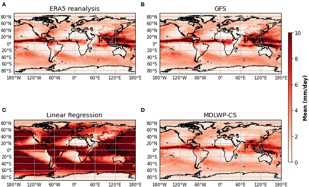
Figure 2. Mean of daily global precipitation corresponding to the (A) ERA5 reanalysis, (B) GFS, (C) linear regression, and (D) MDLWP-CS. The values are shown for the test period 2012–2015.

Figure 3 shows the bias in mean climatology (climatology from forecasted precipitation minus climatology from ERA5 reanalysis) of global precipitation fields from the GFS, MDLWP-CS, and linear regression models for the test period 2012–2015. The linear regression models show excessive wet bias globally. The overall pattern of bias among GFS and MDLWP-CS is similar; however, MDLWP-CS has a dry bias over the ocean in tropical areas. Over the land, there are some notable differences, such as MDLWP-CS showing a slightly dry bias over the Eastern Pacific, whereas over the Sahel region GFS has a wet bias. Moreover, MDLWP-CS performs similarly or better compared to GFS in North and South America. MDLWP-CS exhibits a dry bias in north India and a wet bias in south India.

FIGURE 3

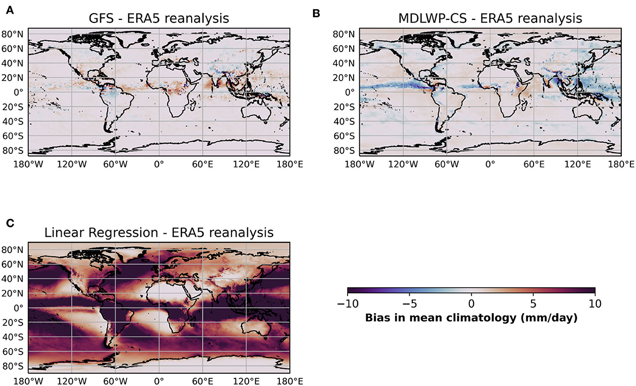
Figure 3. Bias in daily global precipitation corresponding to the (A) GFS, (B) MDLWP-CS, and (C) linear regression. The values are shown for the test period 2012–2015.

The grid-wise temporal correlations (Pearson correlation coefficients) between the ERA5 reanalysis daily precipitation and GFS, MDLWP-CS, and linear regression models have been computed for 2012–2015 and are shown in Figure 4. Linear regression shows nearly zero correlation over most of the global land regions except over equatorial Africa. GFS shows better skill compared to linear regression. However, compared to the benchmark models, the Pearson correlation coefficient values of MDWLP-CS are much higher overall, especially over the land. More precisely, over the land, the GFS shows maximum values of correlation coefficient from 0.2 to 0.3, whereas MDLWP-CS has better correlation in the range of 0.5–0.6. For more clarity, the Pearson correlation coefficients were calculated over eight different regions (Canada, North Asia, Europe, United States, Central Asia, Amazon, Equatorial Africa, and South Asia) for each model and are presented in Table 2. It is noticeable that the correlation coefficient values of MDWLP-CS are much higher compared to GFS and linear regression across all the regions.

FIGURE 4

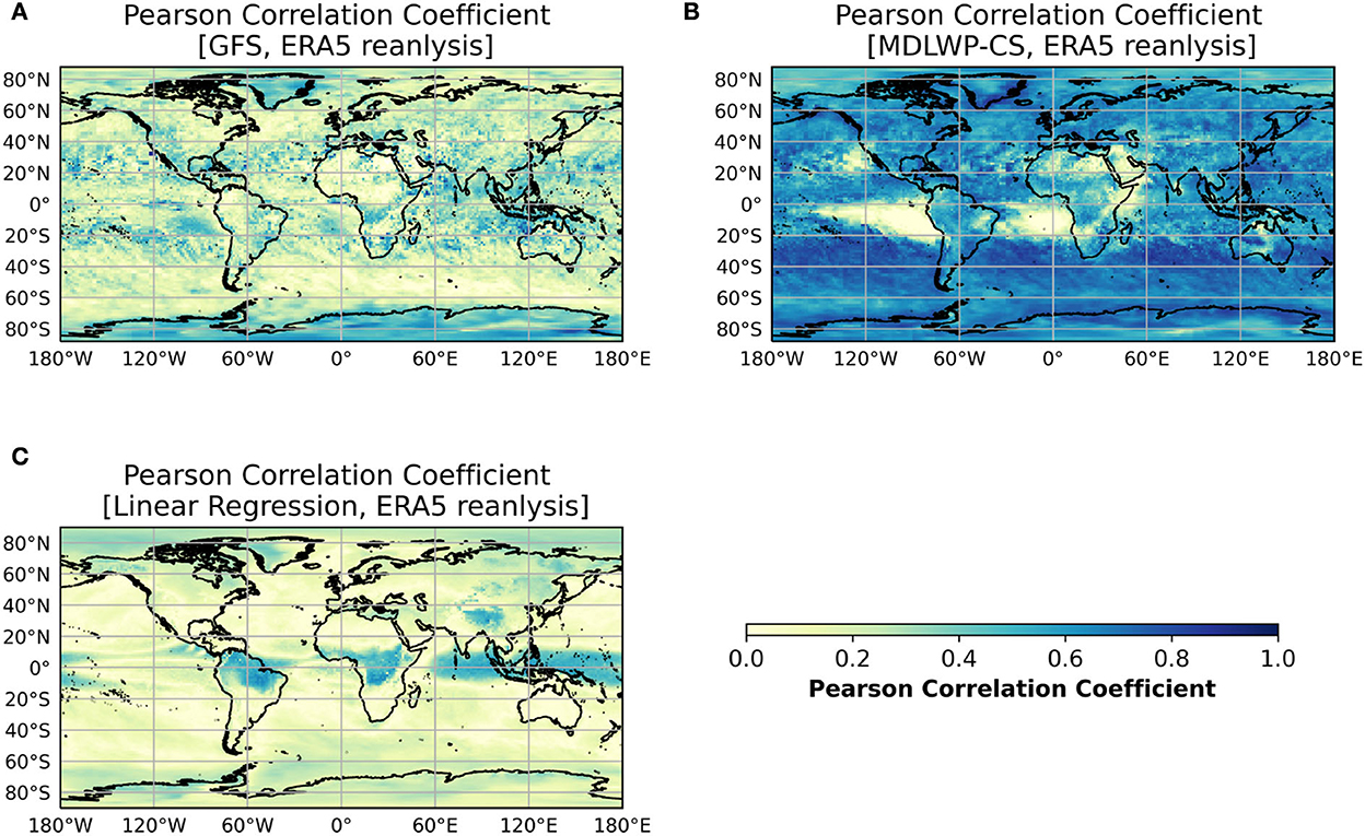
Figure 4. Pearson correlation coefficient of daily global precipitation corresponding to the (A) GFS, (B) MDLWP-CS, and (C) linear regression. The values are shown for the test period 2012–2015.

TABLE 2

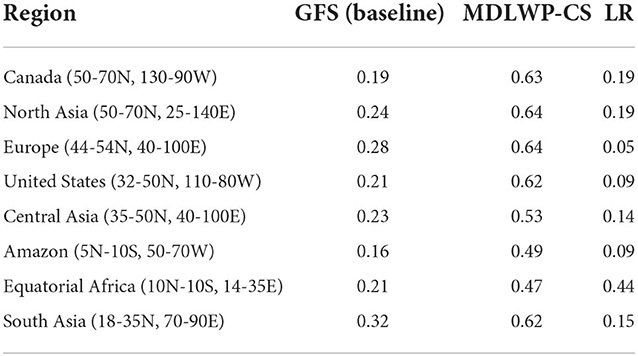
Table 2. Pearson correlation coefficients averaged over different land regions from (a) GFS (baseline), (b) MDLWP-CS, and (c) LR models with ERA5 precipitation for the test years 2012–2015.

For further quantification of the performance of MDWLP-CS compared to GFS, the Critical Success Index (CSI) (Mesinger, 2008) and Index of Agreement (IOA) (Willmott, 1982) are calculated for each of the eight regions. Both the skill scores range from 0 to 1 (where 1 = perfect forecast and 0 = no skill in the forecast). CSI measures the skill of categorical forecast for a particular threshold and is calculated as the ratio of the total number of correct event forecasts (hits) and the total number of forecast, including the number of misses (hits + false alarms + misses). The CSI is not affected by the number of non-event forecasts (correct rejections). The CSI corresponding to 0.5 and 3 mm/day for each of the eight regions are presented in Tables 3, 4, respectively. For both thresholds, the CSI is higher in MDWLP-CS compared to GFS (out of the eight regions, CSI of MDWLP-CS is higher in seven and six regions for 0.5 and 3 mm/day, respectively). The IOA of GFS and MDLWP-CS is presented in Table 5. Furthermore, the skill of MDLWP-CS is better than GFS (out of the eight regions, the IOD of MDWLP-CS is higher in six regions).

TABLE 3

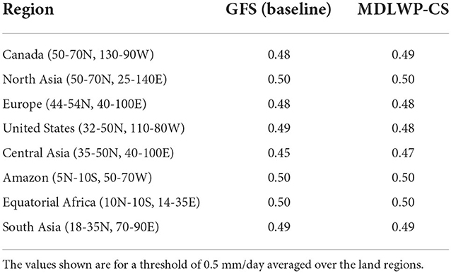
Table 3. Critical success index for the precipitation averaged over different land regions from (a) GFS(baseline) and (b) MDLWP-CS models with ERA5 precipitation for the test years 2012–2015.

TABLE 4

Table 4. Critical success index for the precipitation averaged over different land regions from (a) GFS, (b) MDLWP-CS, and (c) linear regression models with ERA5 precipitation for the test years 2012–2015.

TABLE 5

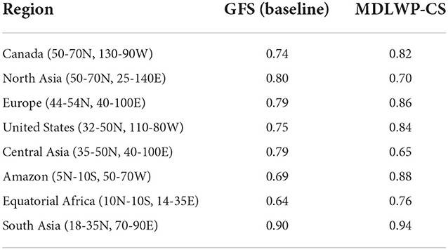
Table 5. Index of agreement for the precipitation averaged over different land regions from (a) GFS and (b) MDLWP-CS models with ERA5 precipitation for the test years 2012–2015.

Overall, the skill of MDLWP-CS is better relative to linear regression and to the operational NWP system (GFS outputs) in terms of predicting daily precipitation. More specifically, the MDLWP-CS is able to model the precipitation reasonably well over the land regions relative to the oceans. It is worth mentioning that in this study, MDLWP-CS uses only a single input, that is, the 2 m surface air temperature with precipitation as the target. This performance can be attributed to the importance of surface air temperature over ocean and land to precipitation (Houston and Niyogi, 2007; Pielke Sr et al., 2007; Routray et al., 2010). MDLWP-CS can preserve the global scale teleconnections due to the cubed sphere transformations and these linkages lead to better performance of the model. Moreover, the skill of the MDLWP-CS will further improve when more precursors of precipitation (such as lower level humidity, wind, and outgoing longwave radiation) are used.

6. Conclusion

In recent years, various efforts have focused on weather prediction using DL, a potent technology to develop DT, to facilitate data-driven simulations of global weather fields as an alternative to NWP. However, there have been limited attempts toward forecasting the global precipitation (diagnostic variables), which is a challenging variable to predict using DL. The Weyn et al. (2019) and Weyn et al. (2020) DL framework for the predicting geopotential height by introducing CS to transform the spherical global data into a temporal mapping algorithm (univariate setup) is built further in this study. We modified the DLWP-CS to transform the architecture from a temporal transformation to a spatio-temporal mapping, wherein precursor(s) of precipitation can be used as input. As a proof of concept, a 2-m surface air temperature is used to predict precipitation using MDLWP-CS and compared with two benchmark models that are linear regression and an operational numerical weather prediction model, GFS. The results highlight the improved skill of MDLWP-CS compared to the benchmark models for predicting daily precipitation. This study thus lays the foundation for using a DL approach for efficient multiscale (regional to global) precipitation forecasting using a parsimonious physics-driven statistical model choice framework. Future efforts are needed to apply this framework for higher impact rainfall events (rather than the climatology alone) and will be pursued in a follow-up study.

Data availability statement

The datasets generated and analyzed for this study can be found in the Zenodo repository: https://doi.org/10.5281/zenodo.6426942.

Author contributions

MS, NA, and DN: conceptualization and methodology. MS: data curation. MS, NA, DN, PP, SJ, SG, and BK: data visualization. MS, NA, DN, and RC: skill verification. All authors writing original draft and approved the final submitted draft.

Funding

This work was benefitted from the National Aeronautics and Space Administration (NASA) Interdisciplinary Science (IDS) 80NSSC20K1262 and 80NSSC20K1268, the National Science Foundation (NSF) Grants for Rapid Response Research (RAPID) AGS 19046442, and the Department of Energy (DOE) Advanced Scientific Computing Research Program Grant No. DE-SC002221.

Acknowledgments

The authors acknowledge the use of high-performance computational resources at Texas Advanced Computing Center (TACC) at The University of Texas at Austin for providing HPC and visualization resources that have contributed to the research results reported in this paper. Further, the facility at IITM, particularly the NVIDIA Tesla P100 GPU is duly acknowledged. DN acknowledges William Stamps Farish Chair endowment through the Jackson School of Geosciences, The University of Texas at Austin.

Conflict of interest

The authors declare that the research was conducted in the absence of any commercial or financial relationships that could be construed as a potential conflict of interest.

Publisher's note

All claims expressed in this article are solely those of the authors and do not necessarily represent those of their affiliated organizations, or those of the publisher, the editors and the reviewers. Any product that may be evaluated in this article, or claim that may be made by its manufacturer, is not guaranteed or endorsed by the publisher.

References

Arcomano, T., Szunyogh, I., Pathak, J., Wikner, A., Hunt, B. R., and Ott, E. (2020). A machine learning-based global atmospheric forecast model. Geophys. Res. Lett. 47, e2020GL087776. doi: 10.1029/2020GL087776

CrossRef Full Text | Google Scholar

Bihlo, A. (2021). A generative adversarial network approach to (ensemble) weather prediction. Neural Networks 139, 1–16. doi: 10.1016/j.neunet.2021.02.003

PubMed Abstract | CrossRef Full Text | Google Scholar

Bihlo, A., and Popovych, R. O. (2022). Physics-informed neural networks for the shallow-water equations on the sphere. J. Comput. Phys. 456, 111024. doi: 10.1016/j.jcp.2022.111024

CrossRef Full Text | Google Scholar

Dimri, A., and Niyogi, D. (2013). Regional climate model application at subgrid scale on indian winter monsoon over the western himalayas. Int. J. Climatol. 33, 2185–2205. doi: 10.1002/joc.3584

CrossRef Full Text | Google Scholar

Espeholt, L., Agrawal, S., Sønderby, C., Kumar, M., Heek, J., Bromberg, C., et al. (2021). Skillful twelve hour precipitation forecasts using large context neural networks. arXiv preprint arXiv:2111.07470. doi: 10.1038/s41467-022-32483-x

PubMed Abstract | CrossRef Full Text | Google Scholar

Han, Y., Zhang, G. J., Huang, X., and Wang, Y. (2020). A moist physics parameterization based on deep learning. J. Adv. Model. Earth Syst. 12, e2020MS002076. doi: 10.1029/2020MS002076

CrossRef Full Text | Google Scholar

Houston, A. L., and Niyogi, D. (2007). The sensitivity of convective initiation to the lapse rate of the active cloud-bearing layer. Mon. Weather Rev. 135, 3013–3032. doi: 10.1175/MWR3449.1

CrossRef Full Text | Google Scholar

Kidd, C., Dawkins, E., and Huffman, G. (2013). Comparison of precipitation derived from the ecmwf operational forecast model and satellite precipitation datasets. J. Hydrometeorol. 14, 1463–1482. doi: 10.1175/JHM-D-12-0182.1

CrossRef Full Text | Google Scholar

Lavers, D. A., Harrigan, S., and Prudhomme, C. (2021). Precipitation biases in the ecmwf integrated forecasting system. J. Hydrometeorol. 22, 1187–1198. doi: 10.1175/JHM-D-20-0308.1

CrossRef Full Text | Google Scholar

LeCun, Y., Bottou, L., Bengio, Y., and Haffner, P. (1998). Gradient-based learning applied to document recognition. Proc. IEEE 86, 2278–2324. doi: 10.1109/5.726791

CrossRef Full Text | Google Scholar

Maher, P., Vallis, G. K., Sherwood, S. C., Webb, M. J., and Sansom, P. G. (2018). The impact of parameterized convection on climatological precipitation in atmospheric global climate models. Geophys. Res. Lett. 45, 3728–3736. doi: 10.1002/2017GL076826

CrossRef Full Text | Google Scholar

Mesinger, F. (2008). Bias adjusted precipitation threat scores. Adv. Geosci. 16, 137–142. doi: 10.5194/adgeo-16-137-2008

CrossRef Full Text | Google Scholar

Pielke Sr, R. A., Adegoke, J., BeltraáN-Przekurat, A., Hiemstra, C. A., Lin, J., Nair, U. S., et al. (2007). An overview of regional land-use and land-cover impacts on rainfall. Tellus B 59, 587–601. doi: 10.1111/j.1600-0889.2007.00251.x

CrossRef Full Text | Google Scholar

Prasad, V., Mohandas, S., Gupta, M. D., Rajagopal, E., and Dutta, S. (2011). Implementation of upgraded global forecasting systems (t382l64 and t574l64) at ncmrwf. NCMRWF Technical Report.

Rao, S. A., Goswami, B., Sahai, A. K., Rajagopal, E., Mukhopadhyay, P., Rajeevan, M., et al. (2019). Monsoon mission: a targeted activity to improve monsoon prediction across scales. Bull. Am. Meteorol. Soc. 100, 2509–2532. doi: 10.1175/BAMS-D-17-0330.1

CrossRef Full Text | Google Scholar

Rasp, S., Dueben, P. D., Scher, S., Weyn, J. A., Mouatadid, S., and Thuerey, N. (2020). Weatherbench: a benchmark data set for data-driven weather forecasting. J. Adv. Model. Earth Syst. 12, e2020MS002203. doi: 10.1029/2020MS002203

CrossRef Full Text | Google Scholar

Rasp, S., and Lerch, S. (2018). Neural networks for postprocessing ensemble weather forecasts. Mon. Weather Rev. 146, 3885–3900. doi: 10.1175/MWR-D-18-0187.1

CrossRef Full Text | Google Scholar

Ravuri, S., Lenc, K., Willson, M., Kangin, D., Lam, R., Mirowski, P., et al. (2021). Skilful precipitation nowcasting using deep generative models of radar. Nature 597, 672–677. doi: 10.1038/s41586-021-03854-z

PubMed Abstract | CrossRef Full Text | Google Scholar

Routray, A., Mohanty, U., Rizvi, S., Niyogi, D., Osuri, K. K., and Pradhan, D. (2010). Impact of doppler weather radar data on numerical forecast of indian monsoon depressions. Q. J. R. Meteorol. Soc. 136, 1836–1850. doi: 10.1002/qj.678

CrossRef Full Text | Google Scholar

Scher, S. (2018). Toward data-driven weather and climate forecasting: approximating a simple general circulation model with deep learning. Geophys. Res. Lett. 45, 12–616. doi: 10.1029/2018GL080704

CrossRef Full Text | Google Scholar

Scher, S., and Messori, G. (2019). Weather and climate forecasting with neural networks: using general circulation models (gcms) with different complexity as a study ground. Geosci. Model Dev. 12, 2797–2809. doi: 10.5194/gmd-12-2797-2019

CrossRef Full Text | Google Scholar

Sønderby, C. K., Espeholt, L., Heek, J., Dehghani, M., Oliver, A., Salimans, T., et al. (2020). Metnet: a neural weather model for precipitation forecasting. arXiv preprint arXiv:2003.12140. doi: 10.48550/arXiv.2003.12140

CrossRef Full Text | Google Scholar

Weyn, J. A., Durran, D. R., and Caruana, R. (2019). Can machines learn to predict weather? using deep learning to predict gridded 500-hpa geopotential height from historical weather data. J. Adv. Model. Earth Syst. 11, 2680–2693. doi: 10.1029/2019MS001705

CrossRef Full Text | Google Scholar

Weyn, J. A., Durran, D. R., and Caruana, R. (2020). Improving data-driven global weather prediction using deep convolutional neural networks on a cubed sphere. J. Adv. Model. Earth Syst. 12, e2020MS002109. doi: 10.1029/2020MS002109

CrossRef Full Text | Google Scholar

Willmott, C. J. (1982). Some comments on the evaluation of model performance. Bull. Am. Meteorol. Soc. 63, 1309–1313. doi: 10.1175/1520-0477(1982)063andlt;1309:SCOTEOandgt;2.0.CO;2

CrossRef Full Text | Google Scholar

Yano, J.-I., Ziemiański, M. Z., Cullen, M., Termonia, P., Onvlee, J., Bengtsson, L., et al. (2018). Scientific challenges of convective-scale numerical weather prediction. Bull. Am. Meteorol. Soc. 99, 699–710. doi: 10.1175/BAMS-D-17-0125.1

CrossRef Full Text | Google Scholar

Yuval, J., and O'Gorman, P. A. (2020). Stable machine-learning parameterization of subgrid processes for climate modeling at a range of resolutions. Nat Commun. 11, 1–10. doi: 10.1038/s41467-020-17142-3

PubMed Abstract | CrossRef Full Text | Google Scholar

Yuval, J., O'Gorman, P. A., and Hill, C. N. (2021). Use of neural networks for stable, accurate and physically consistent parameterization of subgrid atmospheric processes with good performance at reduced precision. Geophys. Res. Lett. 48, e2020GL091363. doi: 10.1029/2020GL091363

CrossRef Full Text | Google Scholar

Zeiler, M. D., and Fergus, R. (2014). “Visualizing and understanding convolutional networks,” in European Conference on Computer Vision (Springer), 818–833.