Evaluation of a global ocean reanalysis generated by a global ocean data assimilation system based on a four-dimensional variational (4DVAR) method

Japan Meteorological Agency (JMA) started to use a new global ocean data assimilation system for the operational seasonal predictions in February 2022. The system is composed of two subsystems with non-eddy-permitting (lower) and eddy-permitting (higher) resolutions. The lower-resolution subsystem adopts a four-dimensional variational (4DVAR) method to optimize the temperature and salinity fields, and the data-assimilated fields are downscaled into the higher-resolution subsystem using incremental analysis updates. The impact of introducing the 4DVAR method in the new ocean data assimilation system is investigated through the comparison of a regular reanalysis run of the system using the 4DVAR method with another run using a three-dimensional variational (3DVAR) method. A comparison of the temperature fields before the downscaling between the two reanalysis runs indicates that the 4DVAR method can more effectively reduce the misfits between the model field and assimilated observation data. However, the increase of the temperature root mean square difference (RMSD) relative to independent Argo float data, along with the larger variance, for the run with the 4DVAR method reveals that the 4DVAR method adjusts the temperature field more significantly but the adjustments are inconsistent with the independent data due to insufficient model physics and resolution. The increase of the RMSD is mitigated after the assimilated fields are downscaled into the higher-resolution subsystem. The 4DVAR method reduces the bias and RMSD of temperature relative to the independent data along the thermocline, as well as near the surface, in the equatorial vertical section, which is expected to affect the prediction of El Niño-Southern Oscillation (ENSO).

1. Introduction

Japan Meteorological Agency (JMA) started to use a new global ocean data assimilation system, MOVE/MRI.COM-G3 in February 2022. The system is a component of the JMA's Coupled Prediction System 3 (CPS3; Hirahara et al., in press), and provides oceanic initial conditions for the coupled atmosphere-ocean general circulation model which also composes CPS3. The prediction results of the coupled model are used for the JMA's seasonal forecasts. In addition, the predicted sea surface temperature (SST) field is provided to the atmospheric Global Ensemble Prediction System (GEPS; JMA, 2022) for the predictions of 1 week to 1 month lead time in JMA.

MOVE/MRI.COM-G3 is composed of the non-eddy-permitting (lower-resolution) subsystem MOVE-G3A, and the eddy-permitting (higher-resolution) subsystem, MOVE-G3F. Temperature, salinity, and sea surface height observations are directly assimilated into MOVE-G3A through a four-dimensional variational (4DVAR) method, and the data-assimilated temperature and salinity fields are downscaled into MOVE-G3F through incremental analysis updates (IAU; Bloom et al., 1996). The 4DVAR method and the downscaling strategy mostly follow those applied to JMA's operational systems for ocean forecasting around Japan (Usui et al., 2015; Hirose et al., 2019).

A feature of MOVE/MRI.COM-G3 is its use of the 4DVAR method. Several weather centers operate global ocean data assimilation systems to provide oceanic initial conditions in their coupled predictions. However, to our best knowledge, 4DVAR methods are not used in those systems. For example, NEMOVAR (Weaver et al., 2005) in the configuration based on a three-dimensional variational (3DVAR) method with first-guess at appropriate time (FGAT) is used in the European Center for Medium-Range Weather Forecasts (Zuo et al., 2019), the UK Met Office (Waters et al., 2015), and the Australian Bureau of Meteorology (Hudson et al., 2017). The US National Center for Environment Prediction adopted a weakly coupled atmosphere-ocean data assimilation system for seasonal forecasting, and the system employs a 3DVAR data assimilation scheme for the ocean component (Xue et al., 2011). The Local Ensemble Transform Kalman Filter is also used in the coupled forecast system of the US National Aeronautics and Space Administration (Hackert et al., 2020).

A 4DVAR method is expected to generate analysis fields more consistent with the ocean physics than 3DVAR methods because it can use an ocean model as physical constraints. In particular, if only the initial fields, atmospheric forcing, and uncertain parameters used in physical parameterizations are adjusted with observations in a long assimilation window using a 4DVAR method, a model trajectory which totally follows the model physics and is consistent with the observations can be obtained for the window. In addition, using a long assimilation window has an advantage that wider range of observations can be used to obtain analysis values at each time and location.

Because of these reasons, ocean state estimation has been performed using 4DVAR methods with long assimilation windows of 1 year to several decades (e.g., Mazloff et al., 2010; Forget et al., 2015; Köhl, 2015; Osafune et al., 2015). The coupled ocean-atmosphere 4DVAR system developed by the JAMSTEC K-7 group also applies 9-month assimilation windows (Sugiura et al., 2008). Ocean states estimated by these approaches have been also used for the seasonal-to-decadal coupled predictions on a research basis (e.g., Pohlmann et al., 2009; Mochizuki et al., 2016). However, use of long assimilation windows does not allow to provide oceanic initial conditions in the near real-time at short (preferably 1-day) interval, and therefore not suitable for operational coupled predictions.

In the numerical weather predictions, atmospheric initial conditions are provided by the sequential implementation of 4DVAR analysis with short (typically six-hour) assimilation windows. Relatively short assimilation windows are also used in 4DVAR systems for coastal and regional seas (e.g., Moore et al., 2011; Hirose et al., 2019). In the context of seasonal predictions, a study by Vialard et al. (2003) and Weaver et al. (2003) applied a 4DVAR method with 10- and 30-day assimilation windows to a non-eddy-permitting model, and assessed its advantage over a 3DVAR method with respect to the reproducibility in the tropical Pacific. They demonstrated that the 4DVAR method reduces misfits from the assimilated data in comparison with the 3DVAR method. However, the feasibility of 4DVAR methods with short assimilation windows for ocean initialization for coupled predictions has not yet been fully explored.

In this study, we aim to demonstrate the benefits of introducing a 4DVAR method to a global ocean data assimilation system with the resolution and the length of the assimilation windows applicable for operational coupled predictions. We conduct a 4DVAR reanalysis run with 10-day assimilation windows using MOVE/MRI.COM-G3, and compare the result with the 3DVAR version of the reanalysis run. The quality of the two reanalysis runs will be assessed through the consistency of the temperature fields at the surface and 100 m depth, and in the equatorial vertical section with objective mapping of sea surface temperature (SST) and Argo float profiles.

The rest of this paper is organized as follows: Section 2 introduces the configuration of MOVE/MRI.COM-G3; Section 3 describes the setup of the two reanalysis runs and the statistical metrics used to evaluate the analysis fields; Section 4 compares the two reanalysis runs and examine the effects of introducing the 4DVAR method; Section 5 provides a summary and remaining discussion.

2. System configuration of MOVE/MRI.COM-G3

2.1. Lower-resolution subsystem: MOVE-G3A

2.1.1. Forward and adjoint models

The lower-resolution subsystem, MOVE-G3A, generates ocean analysis fields mainly based on a 4DVAR method using a global ocean model and its adjoint model. The main specification of the original (forward) model used in the subsystem is summarized in Table 1. The forward and adjoint models adopt a tripolar grid (Murray, 1996) over the global domain with a zonal resolution of 1° and the meridional resolution of 0.3°-0.5° with refinement near the equator. They have 60 vertical layers and a bottom boundary layer (Nakano and Suginohara, 2002). The nominal depths of 24 upper layers are 1, 3.5, 6.5, 10, 15, 22, 30.5 m and every 10 m between 40 and 200 m, and that of the lowest layer is 6,150 m. Those models are constructed with the original and adjoint codes of the MRI Community Ocean Model (MRI.COM) Version 4 (Tsujino et al., 2017). The codes are basically the same as those used in JMA's current operational system for ocean forecasting around Japan (Hirose et al., 2019), but MOVE-G3A uses different options due to the difference of the grid coordinate and the lower horizontal resolution.

TABLE 1

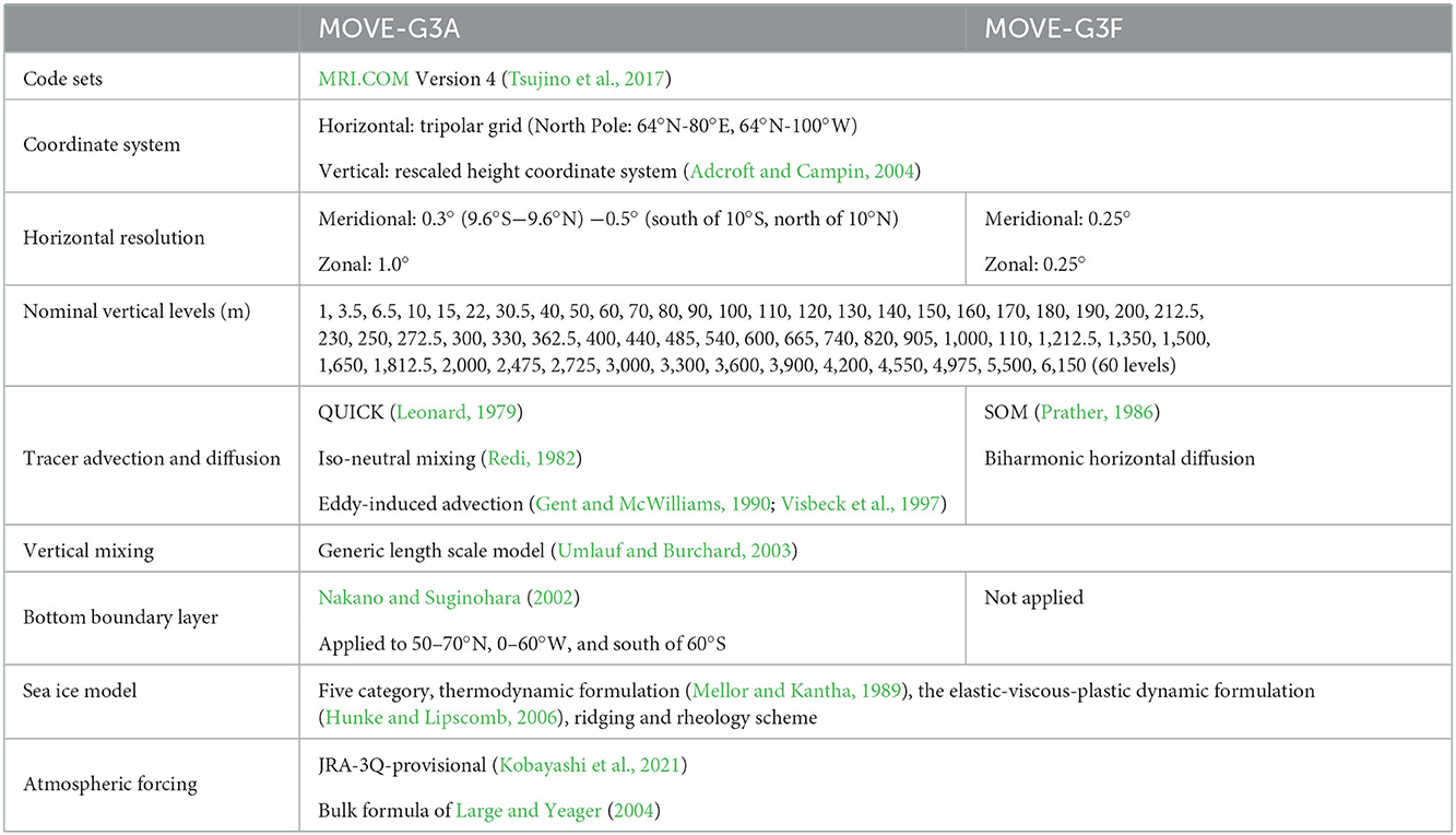
Table 1. Main specification of the ocean models used in MOVE-G3A and MOVE-G3F.

The forward model uses the QUICK tracer advection scheme (Leonard, 1979). The second-order moments scheme of Prather (1986), applied in the higher-resolution subsystem, is not used in MOVE-G3A because it considerably increases the quantity of data that must be stored in memory to execute the adjoint model. In the forward model, the layer thicknesses vary small because the rescaled height coordinates system (Adcroft and Campin, 2004) is applied, and diffusion and viscosity coefficients vary due to physical parameterizations, including iso-neutral mixing (Redi, 1982) and eddy-induced advection (Gent and McWilliams, 1990; Visbeck et al., 1997) parameterizations and the vertical mixing scheme based on the generic length scale model (Umlauf and Burchard, 2003). A five-category sea-ice model, based on the thermodynamic formulation of Mellor and Kantha (1989) and the elastic-viscous-plastic dynamic formulation of Hunke and Lipscomb (2006) with a ridging and rheology scheme, is also incorporated. The forward model uses atmospheric forcing estimated from a provisional version of the Japanese Reanalysis for Three-Quarters of a Century (JRA-3Q-provisional; Kobayashi et al., 2021) using the bulk formula of Large and Yeager (2004). JRA-3Q is the new atmospheric reanalysis dataset generated in JMA.

The tangent linear model is generated by linearizing the ocean model under some approximations for avoiding instability and singularity as done in Fujii et al. (2008). For example, the deviations of the vertical layer thicknesses and sea ice parameters from its background state caused by the perturbation of the model prognostic fields are ignored. We also ignore the change of the zonal and vertical diffusion coefficients determined by the iso-neutral mixing and eddy-induced advection parameterizations and the vertical mixing scheme due to the perturbation, and the sensitivities of sea-ice parameters. In contrast, the operator equivalent to the exact transpose matrix of the tangent linear model is composed as the adjoint model. The consistency of the tangent linear and adjoint models is validated by checking that (LΔx)^T(LΔx) = Δx^T(L^TLΔx) is satisfied, where Δx denotes the perturbation of the prognostic fields, and L and L^T are tangent linear and adjoint models.

2.1.2. 4DVAR method

In MOVE-G3A, a 4DVAR analysis is performed through iterative integrations of forward and adjoint models in an assimilation window of 10 days, and analysis increments are applied to the temperature, salinity, and sea ice concentration (SIC) fields in the first half (5 days) of the assimilation window (Figure 1). The increments are gradually added to the corresponding prognostic fields during the integration of the forward model in the application period according to the following equation,

$\begin{array}{ll}{\text{x}}_{t+1}=M({\text{x}}_t)+\widehat{\text{d}}/L,& (1)\end{array}$

where M is the nonlinear model operator, x_t is the prognostic fields, t is the counter of the time step, $\widehat{\text{d}}$ is the analysis increments, and L is the number of the time steps in the application period. The increments are estimated from the observation data in the second half of the assimilation window (i.e., the observation window is between the sixth and tenth days of the assimilation window). The SIC increments are determined through a 3DVAR analysis at first and the temperature and salinity increments are estimated later through the 4DVAR analysis. The SIC increments are applied in the model integrations during the 4DVAR analysis. Here, sea ice parameters other than SIC and the sea surface air temperature and humidity, which are used for the calculation of the atmospheric forcing, are also modified depending on the SIC correction using a method generally based on Toyoda et al. (2016).

FIGURE 1

Figure 1. Schematic figure of the data assimilation process of MOVE/MRI.COM-G3.

The temperature and salinity increments are expressed by a linear combination of coupled temperature and salinity vertical Empirical Orthogonal Function (EOF) modes set for each subdomain of the model domain, as in Fujii and Kamachi (2003a). That is, the vertical profiles of the temperature and salinity increments at each horizontal grid point, d_p, is written as follows,

$\begin{array}{ll}{\text{d}}_p={\text{b}}_p+{\displaystyle {\sum }_n}{\displaystyle {\sum }_m}{a}_{n,p}{w}_{n,m,p}{\lambda }_{n,m}{\text{S}}_p{\text{u}}_{n,m},& (2)\end{array}$

where n and m are the indices of subdomains and EOF modes, u_n,m and λ_n,m are the EOF mode and the square root of the corresponding eigen value, w_n,m,p is the amplitude of the EOF modes, b_p denotes vertical profiles of temperature and salinity biases, and S_p is the diagonal matrix whose diagonal components are the standard errors of temperature and salinity at each depth. Each subdomain is overlapped at the boundary to avoid discontinuities in the analysis increment fields and a_n,p is the weight of each subdomain at the point. Here, u_n,m, λ_n,m, S_p, are prescribed from past observations included in World Ocean Database 2018 (Boyer et al., 2018) and Global Temperature and Salinity Profile Program (GTSPP; Hamilton, 1994) and the climatological fields in the World Ocean Atlas 2018 (Locarnini et al., 2019; Zweng et al., 2019). The biases updated in the previous analysis by the method of Balmaseda et al. (2007) are used as b_p (see also Fujii et al., 2009). Then, w_n,m,p is the parameter adjusted by the 4DVAR method. The transformation of (2) is performed at the grid points of the analysis grid in a polar coordinate system different from the model grid, and then transformed to the model grid. The conversions can be summarized in a single equation as follows:

$\begin{array}{ll}\text{d}=\text{T}(\text{b}+\text{SU}\Lambda \text{Aw})=\text{T}\text{b}+\text{G}\text{w},& (3)\end{array}$

where, d denotes the temperature and salinity analysis increment fields in the model grid, T denotes the conversion from the analysis grid to the model grid, b denotes the bias fields in the analysis grid, S is the diagonal matrix with standard errors of temperature and salinity at each grid point as diagonal components, U is a matrix composed of the column vectors in which u_n,m is given to the components corresponding to each horizontal grid point and zero is given to the rest, and Λ and A are diagonal matrices whose components are λ_n,m and a_n,p, respectively, w is the vector of w_n,m,p, and G=TSU Λ A.

The amplitudes of the EOF modes are determined by minimizing the following cost function J in the 4DVAR methods,

$\begin{array}{ll}J=J_b+J_{T,S}+J_{\Delta h},& (4)\end{array}$

where

$\begin{array}{ll}{J}_b={\frac{1}{2}\text{w}}^T{\text{B}}^{-1}\text{w}+\frac{1}{2}{\left(\frac{\eta -{\eta }_b}{{\sigma }_{\eta }}\right)}^2,& (5)\end{array}$

$\begin{array}{ll}{J}_{T,S}=\frac{1}{2}{(\text{H}\overline{\text{x}}-\text{y})}^T{\text{R}}^{-1}(\text{H}\overline{\text{x}}-\text{y}),& (6)\end{array}$

$\begin{array}{ll}{J}_{\Delta h}=\frac{1}{2}{(\Delta \text{h}-{\text{y}}_{\Delta h})}^T{\text{R}}_{\Delta h}^{-1}(\Delta \text{h}-{\text{y}}_{\Delta h}).& (7)\end{array}$

The first term J_b is the constraint to the background, and B is the correlation matrix of w in which the correlation between different modes is set to zero and the horizontal correlation between the same mode follows a Gaussian function of the distance between two points. The parameter η is the globally uniform sea level adjustment associated with the uncertainty of the change of freshwater amount in the global ocean, and it is estimated along with w. Estimation of η in the previous analysis is used as the background value, η_b, and σ_η is the prescribed standard error of η_b. The second term J_T,S is the constraint to temperature and salinity observations including gridded SST data, where y is the vector of temperature and salinity observations, R is its error covariance matrix. Here,

$\begin{array}{ll}\overline{\text{x}}=\overline{M}(\text{d})=\overline{M}(\text{G}\text{w }+\text{ T}\text{b}),& (8)\end{array}$

where $\overline{M}$ is the operator to generate four-dimensional temperature and salinity fields by integrating the forward model with applying d as the analysis increments. The observation matrix H denotes the conversions from the four-dimensional fields to each observation. The third term J_Δh is the constraint to the Sea Level Anomaly (SLA) observations, where y_Δh is the vector of SLA observations, and R_Δh is its error covariance matrix. Here, Δh is the SLA calculated from $\overline{\text{x}}$ and written as

$\begin{array}{ll}\Delta \text{h}=D(\overline{\text{x}})-{\text{h}}_m+{\Delta \text{h}}_c+\eta 1,& (9)\end{array}$

where D is the operator denoting the calculation of the sea surface dynamic height at the observation points from four-dimensional temperature and salinity fields, and h_m denotes mean dynamic height. The vector Δh_c denotes the correction to the dynamic height anomaly in order to account for the increase in the freshwater amount in the global ocean due to global warming and the seasonal variation of pressure at the reference depth for the dynamic height calculation (2,000 m) presented by Kuragano et al. (2014). The vector 1 is the vector whose elements are all 1's.

The gradient of the cost function along w is calculated by the following equations:

$\begin{array}{ll}{\nabla }_{\text{w}}J={\text{B}}^{-1}\text{w}+{\text{G}}^T{\text{M}}^T{\nabla }_{\overline{\text{x}}}J,& (10)\end{array}$

where

$\begin{array}{ll}{\nabla }_{\overline{\text{x}}}J={\text{H}}^T{\text{R}}^{-1}(\text{H}\overline{\text{x}}-\text{y})+{\text{D}}^T{\text{R}}_{\Delta h}^{-1}(\Delta \text{h}-{\text{y}}_{\Delta h})& (11)\end{array}$

and G^T, ${\overline{\text{M}}}^T$, H^T, and D^T denote the adjoint operators of G, $\overline{M}$, H, and D. The inclusion of ${\overline{\text{M}}}^T$ in the left-hand side of Equation (10) means that the backward integration of the adjoint model is required to compute the gradient of the cost function. Then, the gradient of the cost function along η is written as follows:

$\begin{array}{ll}{\nabla }_{\eta }J=\frac{\eta -{\eta }_b}{{{\sigma }_{\eta }}^2}+1^T{\text{R}}_{\Delta h}^{-1}(\Delta \text{h}-{\text{y}}_{\Delta h}).& (12)\end{array}$

In addition, modifications to avoid the density inversion and extremely low temperature and to perform a variational quality control are applied to the cost function (Fujii et al., 2005; Usui et al., 2011).

The cost function is minimized by a quasi-Newton Method (Fujii and Kamachi, 2003b; Fujii, 2005). In the minimization, the computation of the cost function, including the integration of the forward model, and the computation of the gradient, including the backward integration of the adjoint model is repeated.

After a 4DVAR analysis is completed, a subsequent 4DVAR analysis is conducted using the 10 days from the center of the previous assimilation window as the new assimilation window. The second half of the assimilation window in a 4DVAR analysis is thus overlapped with the first half of the subsequent 4DVAR analysis, and the 4DVAR analysis fields in the second half of the assimilation window are updated again by the subsequent 4DVAR analysis. In this study, we consider the 4DVAR analysis fields in the second half of the assimilation window before updated by the subsequent 4DVAR again as the analysis fields for MOVE-G3A because the subsequent analysis uses observed data up to 5 days into the future, and therefore lags behind the real-time by more than 5 days.

2.2. Higher-resolution subsystem: MOVE-G3F

Temperature and salinity analysis fields in MOVE-G3A (the 4DVAR analysis fields in the second half of the assimilation window) are downscaled into the higher-resolution system, MOVE-G3F, through IAU (Figure 1). The configuration of the model used in MOVE-G3F (See Table 1) are the same as those of the forward model in MOVE-G3A, except for a few items listed below. First, the horizontal resolution is 0.25° × 0.25°. Second, the bottom boundary layer is not applied. Third, the SOM tracer advection scheme is applied instead of the QUICK scheme. Fourth, biharmonic horizontal diffusion parametrization is applied in place of the parameterizations of iso-neutral mixing and eddy-induced advection.

In the downscaling, a prediction by the higher-resolution model for the second half of the assimilation window (i.e., the 5 days from the sixth to tenth days) of MOVE-G3A is conducted from the downscaled analysis fields at the end of the previous assimilation window. The increments are then calculated by subtracting the means of the predicted temperature and salinity from the means of temperature and salinity analyzed by MOVE-G3A. Finally, these increments are gradually added to MOVE-G3F for the 5 days through Equation (1). The higher-resolution model fields at the end of the assimilation window that is consequently calculated by the downscaling are used as oceanic initial conditions for coupled model predictions. The analysis increments of SIC are also estimated through the same 3DVAR analysis as in MOVE-G3A, and gradually added to the model along with the temperature and salinity increments. Other sea ice parameters are also adjusted for the SIC increments by the same method as in MOVE-G3A.

3. Experimental setting and metrics

3.1. Setting of reanalysis runs

In this study, we conduct two reanalysis runs, named the 4DVAR and 3DVAR Runs, and examine the impact of introducing the 4DVAR method by comparing the accuracy of the temperature fields in the reanalysis runs. The 4DVAR Run is the reanalysis run of MOVE-G3 (including MOVE-G3A and MOVE-G3F) with the operational configuration described in the previous section, and therefore the run applies the 4DVAR method to assimilate observation data into the MOVE-G3A model.

Meanwhile, the configuration is changed for the 3DVAR Run as follows. First, Equation (8) is replaced by

$\begin{array}{ll}\overline{\text{x}}={\overline{\text{x}}}_b+\text{P}\text{d},& (13)\end{array}$

where ${\overline{\text{x}}}_b$ is the four-dimensional temperature and salinity fields over the assimilation window predicted from the result of the previous analysis, and P is the matrix that transforms a three-dimensional field vector into a four-dimensional field vector that persists in that three-dimensional field. The integration of the forward and adjoint models is removed by this replacement, and thus it becomes a 3DVAR analysis. Second, the assimilation window is shortened to 5 days with assimilating observation data in the whole assimilation window, and the optimized increments d are gradually added to the model temperature and salinity fields according to Equation (1) during the whole assimilation window. The SIC 3DVAR analysis is also performed and the SIC increments are applied to the model along with temperature and salinity increments. The subsequent assimilation window is then started from the end of the previous window and therefore the windows are not overlapped with each other. The downscaling by MOVE-G3F is conducted in a regular manner in both the 4DVAR and 3DVAR Runs.

Both reanalysis runs start from January 1, 2004 with the same initial values and continues through December 31, 2014. Common observation data including temperature and salinity profiles, satellite SLA data, and gridded SST and SIC data are assimilated in the reanalysis runs. The temperature and salinity profiles are collected from World Ocean Database 2013 (Boyer et al., 2013) and GTSPP. The SLA data are obtained from AVISO multimission products for TOPEX/Poseidon, Jason-1/2, Envisat, GFO, CryoSat, Altika, and HY-2A (AVISO, 2015). The gridded SST and SIC data are drawn from Merged satellite and in situ Global Daily Sea Surface Temperature (MGDSST) produced by JMA with the 0.25° resolution (Kurihara et al., 2006; Matsumoto et al., 2006). Temperature and salinity profiles of Argo floats whose last digit of the World Meteorological Organization ID is 8 or 9 (i.e., ~20% of Argo data) are withheld from the assimilation in both reanalysis runs, and used for evaluating the accuracies of their temperature fields as independent data. The distribution of the independent Argo data is similar to the distribution of all Argo data, as confirmed in Fujii et al. (2015). SST data below −0.5°C in MGDSST are also discarded in order to prevent undesirable sea ice melting.

3.2. Metrics for accuracy of temperature fields

This study compares the accuracy of the temperature fields at the surface (i.e., SST) and 100-m depth in the two reanalysis runs. As the metrics for accuracy, we calculate biases and root mean square differences (RMSDs) relative to MGDSST or Argo float data for the daily mean temperature fields in the 10-year period of 2005–2014. For the biases and RMSDs relative to MGDSST, data for times and locations where sea ice is present are excluded from the calculation, considering the low reliability of SST data in MGDSST near sea ice. The biases and RMSDs relative to Argo float data are calculated for each 5° (meridional) × 10° (zonal) box using the data observed within the box, and they are calculated separately for the assimilated and the independent Argo float data. In addition, the ratio of the standard deviation (root mean square difference from the mean) of the fields in the reanalysis runs to that of the independent Argo float data (hereafter, relative standard deviation) is calculated for each 5° × 10° box to assess how well the actual variance is represented in the reanalysis runs.

4. Results

4.1. Impacts of 4DVAR on the temperature fields of the lower-resolution subsystem

In this subsection, we investigate the impacts of introducing the 4DVAR analysis by comparing the temperature fields of the lower-resolution subsystem MOVE-G3A in the 4DVAR and 3DVAR Runs. First, the accuracy of the SST fields is evaluated using MGDSST as the reference data. Here, it should be noted that MGDSST is assimilated in the reanalysis runs and is, therefore, not independent data.

Figure 2A shows that in the 4DVAR Run, the bias is generally smaller than 0.02°C in the tropical and subtropical regions except in the central and eastern equatorial Pacific, where a negative bias area down to −0.06°C spreads. In contrast, in the 3DVAR Run (Figure 2B), the negative bias in the eastern equatorial Pacific is more significant, and positive values spreads over wide areas in the western tropical Pacific and eastern tropical Indian Ocean. Noticeable negative biases also appear in the subtropical North Atlantic and the Arabian Sea in the 3DVAR Run. The bias is, thus, significantly reduced in the 4DVAR Run, especially in the tropical areas. Meanwhile, the warm bias over the Antarctic Ocean common in the two reanalysis runs, is mostly caused by not assimilating low SST data from MGDSST. Figure 2C shows that in the 4DVAR Run, the RMSDs are smaller than 0.5°C in most areas except around strong current systems, in the Arctic Ocean, and in some coastal seas. Figure 2D then shows that the RMSDs of the SST analysis values relative to MGDSST are smaller for the 4DVAR Run in most areas except for the Arctic Ocean and some coastal seas.

FIGURE 2

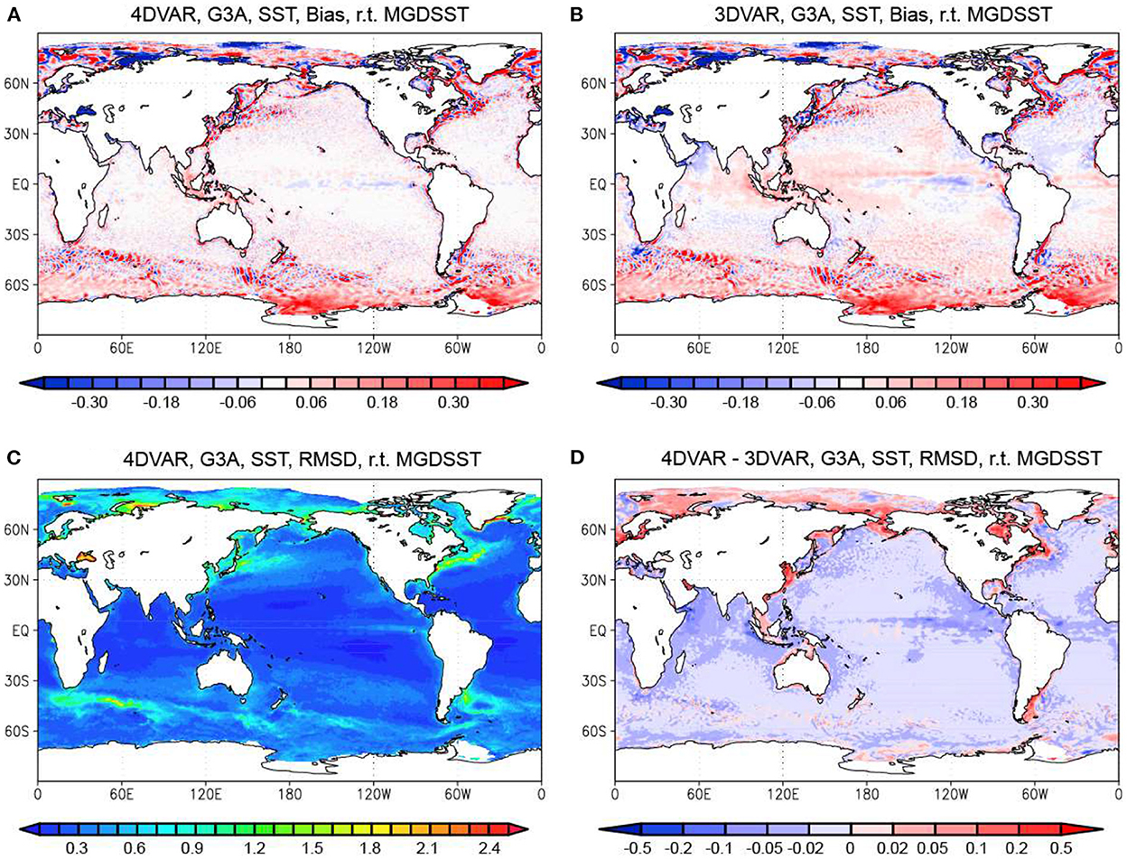
Figure 2. Bias and RMSD of the MOVE-G3A SST for the 4DVAR and 3DVAR Runs relative to MGDSST. (A) Bias in the 4DVAR Run. (B) Bias in the 3DVAR Run. (C) RMSD in the 4DVAR Run. (D) Difference of the RMSDs between the 4DVAR and the 3DVAR Runs. Blue colors in (D) mean that the RMSD is smaller for the 4DVAR Run. Units in °C.

Evaluation using the assimilated Argo float data as the reference also demonstrated that the distribution and variation of near-surface temperature are well recovered by the 4DVAR Run. Figure 3A indicated that the bias of MGDSST relative to the assimilated Argo data is negative for the Southern Ocean except around the Antarctic coast and the North American side of the Arctic Ocean, and positive for the rest of the ocean including the North Pacific, the North Atlantic, and the north-western part of the Indian Ocean. This feature is generally consistent with the bias of the NOAA/NESDIS/NCEI Daily Optimum Interpolation SST (DOISST), version 2.0 (Huang et al., 2021), although the positive bias is more notable in MGDSST. On the other hand, MOVE-G3A SST field in the 4DVAR Run has a warm bias in the most area relative to the assimilated Argo float data (Figure 4A). Thus, the bias in the 4DVAR Run does not directly reflect the bias of MGDSST. Figure 3C, depicting the difference of the absolute value of the SST bias in the 4DVAR Run from the absolute value for MGDSST, indicates that the bias in the 4DVAR Run is smaller than that for MGDSST in the most area except for the subtropical South Atlantic, the eastern subtropical South Pacific, and Antarctic coastal seas. It should be noted that the Argo float data are not used in the production of MGDSST. Assimilating the Argo float data properly reduces the SST bias in the 4DVAR Run.

FIGURE 3

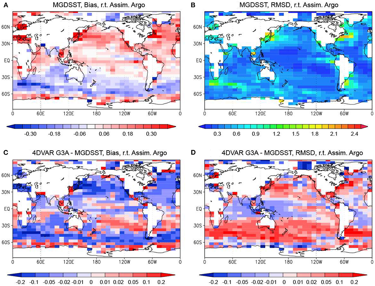
Figure 3. Bias (A) and RMSD (B) of SST data from MGDSST, and differences of bias absolute values (C) and RMSDs (D) of the MOVE-G3A SST for the 4DVAR Run from those for the SST data from MGDSST. The biases and RMSDs are calculated using the assimilated Argo float data as the reference. Blue colors mean that the bias absolute value or the RMSD is smaller for the 4DVAR Run. Units in °C.

FIGURE 4

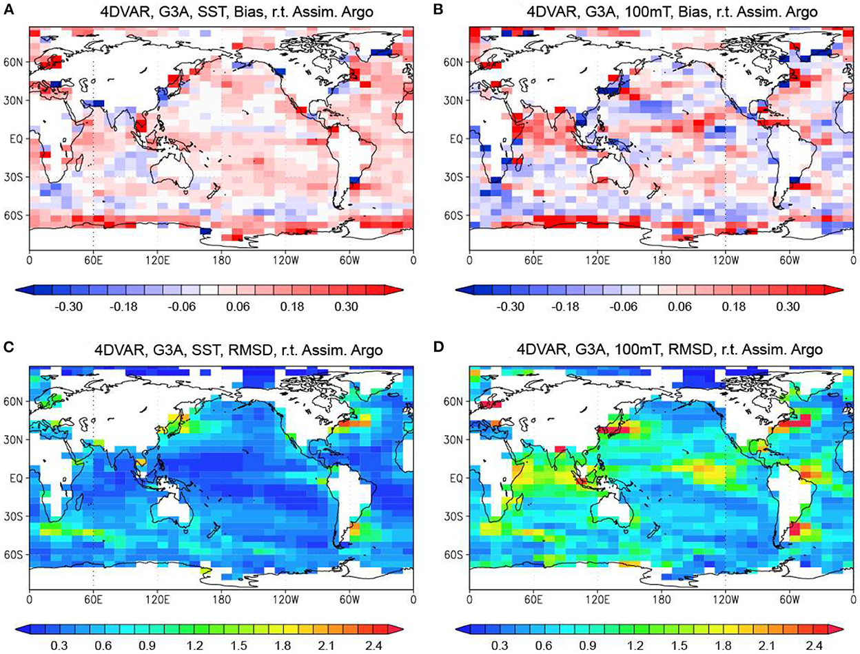
Figure 4. Bias and RMSD of the MOVE-G3A temperature at the surface and 100 m depth in for the 4DVAR Run relative to the assimilated Argo float data. (A, B) Bias at the surface and 100 m depth. (C, D) RMSD at the surface and 100 m depth. Units in °C.

The distribution of RMSD for the MOVE-G3A SST relative to the assimilated Argo float data in the 4DVAR Run (Figure 4C) is similar to the distribution of the RMSD against MGDSST (Figure 2C), and also to the distribution of RMSD of MGDSST against the assimilated Argo float data (Figure 3B), with large values around strong current systems and in some coastal seas. The difference of the RMSD relative to the assimilated Argo float data between the 4DVAR Run and MGDSST (Figure 3D) shows that the SST estimates of the 4DVAR Run are closer to observations than MGDSST in the tropical Indian Ocean, western tropical Pacific, and western tropical Atlantic where SST distribution is relatively smooth, while the 4DVAR Run is less accurate in mid-latitude zones with more eddy activity. This results suggests that the benefit of assimilating the Argo float data is canceled by the insufficient model resolution in the eddy-active areas.

Comparison of the bias absolute value and RMSD for the MOVE-G3A SST against the assimilated Argo float data between the 4DVAR and 3DVAR Runs, as well as the statistics using MGDSST as the reference data, suggests that the 4DVAR scheme more effectively reduces the misfit of the SST field to the assimilated observations. The SST bias is reduced for the 4DVAR Run in most areas except for the North Atlantic (Figure 5A). The RMSD is also found to decrease in large part of the ocean, especially in the equatorial Pacific, Southern Indian and Atlantic Oceans, around the Kuroshio and Gulf Stream (Figure 5C).

FIGURE 5

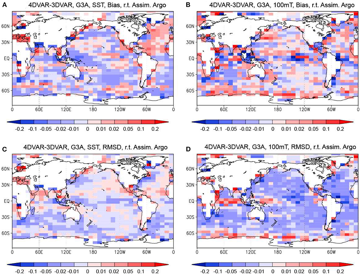
Figure 5. Difference of bias absolute values and RMSDs of the MOVE-G3A temperature relative to the assimilated Argo float data between the 4DVAR and 3DVAR Runs. (A, B) Difference of bias absolute values at the surface and 100 m depth. (C, D) Difference of RMSDs at the surface and 100 m depth. Blue colors mean that the bias absolute value or the RMSD is smaller for the 4DVAR Run. Units in °C.

As for temperature at 100 m depth, the 4DVAR Run has a smaller bias in slightly more boxes, especially in the central tropical Pacific and the western tropical Atlantic, where the bias is smaller by more than 0.1°C (Figure 5B). The RMSD (shown in Figure 4D) has decreased by more than 0.01°C over a wide area, except in the tropical Indian Ocean, western tropical Pacific, and around sea ice (Figure 5D). Thus, the temperatue at the 100 m depth are also better constrained by observation data in the 4DVAR Run.

The distribution of the difference between the 4DVAR and 3DVAR Runs of the bias absolute values relative to the independent Argo float data (not shown) is very similar to that of the difference of the absolute values from the assimilated Argo float data for both surface and 100 m depth (Figures 5A, B), and indicating positive impact of introducing the 4DVAR method. However, the RMSD relative to the independent Argo float data for the 4DVAR Run is larger than that for the 3DVAR Run in many boxes (Figures 6A, B). In particular, a relatively large increase in RMSD due to the application of the 4DVAR method can be seen in the tropical Indian Ocean both at the surface and at the 100 m depth. The RMSD computed using the independent Argo float data, thus, does not clearly confirm the advantage of using the 4DVAR method.

FIGURE 6

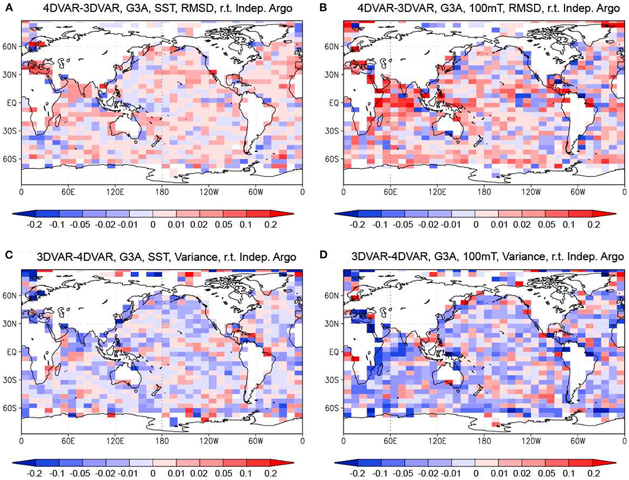
Figure 6. Difference of the RMSDs and the relative standard deviations of the MOVE-G3A temperature relative to the independent Argo float data between the 4DVAR and 3DVAR Runs. (A, B) Difference of the RMSDs at the surface and the 100 m depth. (C, D) Difference of the relative standard deviations at the surface and 100 m depth. Blue colors mean that the RMSD is smaller for the 4DVAR Run in (A, B), and that the relative standar deviation is larger for the 4DVAR Run in (C, D). Units in °C.

It should be noted that in the 4DVAR Run, the relative standard deviation and hence the variance of the temperature are generally larger than in the 3DVAR Run both at the surface and at 100 m depth (Figures 6C, D). Thus, the 4DVAR Run better represents the variance of the temperature field, which is typically underestimated in lower-resolution systems such as MOVE-G3A, by adjusting model fields more significantly to fit the observation data. The larger RMSD in the 4DVAR Run, however, indicates that the adjustment is not well consistent with the real ocean at the locations where observation data are not assimilated probably due to insufficiency of the model resolution and physics.

4.2. Impacts of 4DVAR on the temperature field after downscaling

Next, we investigate the effect of the 4DVAR method on the temperature field downscaled to the 0.25° resolution by MOVE-G3F. Figures 7A, B show the bias of the MOVE-G3F SST relative to MGDSST in the 4DVAR and 3DVAR Runs. Comparing Figure 7A with Figure 2A, warm biases not seen in the MOVE-G3A SSTs appear in the MOVE-G3F SSTs after downscaling in the western tropical Pacific and eastern tropical Indian Ocean. In addition, the cold bias is intensified in the eastern equatorial Pacific, and small cool biases are dominant in other tropical and subtropical regions. The SST bias is, thus, increased by the downscaling. However, a comparison of Figures 7A, B shows that the bias of the MOVE-G3F SST for the 4DVAR Run is still smaller than that for the 3DVAR Run.

FIGURE 7

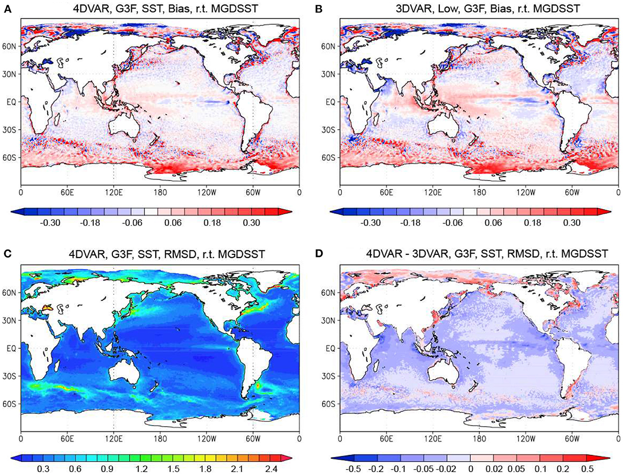
Figure 7. Bias and RMSD of the MOVE-G3F SST for the 4DVAR and 3DVAR Runs relative to MGDSST. (A) Bias in the 4DVAR Run. (B) Bias in the 3DVAR Run. (C) RMSD in the 4DVAR Run. (D) Difference of the RMSDs between the 4DVAR and the 3DVAR Runs. Blue colors in (D) mean that the RMSD is smaller for the 4DVAR Run. Units in °C.

The distribution of RMSD relative to MGDSST in the MOVE-G3F SST in the 4DVAR Run (Figure 7C) shows little difference compared to that for the MOVE-G3A SST (Figure 2C). Comparing the RMSD of the MOVE-G3F SSTs for the 4DVAR and 3DVAR Runs (Figure 7D), the RMSD is smaller for the 4DVAR Run and the difference is larger than for the MOVE-G3A SSTs.

Figures 8A–D depict the differences of the bias absolute values and RMSDs of temperature relative to the independent Argo data between before and after the downscaling in the 4DVAR Run. As for SST, the bias increases in the western tropical Pacific and the equatorial Indian Ocean, but decreases in many other areas. The RMSD also decreases in a relatively large part of the ocean although it increases in the equatorial Pacific and the Southern Ocean. Thus, downscaling usng the higer-resolution system MOVE-G3F improves the reproducibility of SST by resolving finer-scale variability. In contrast, a loss of the physical balance by the downscaling seems to reduce the accuracy of the temperature fields at 100 m depth. The areas where bias for the 100 m temperature decreases and increases are comparable, while the RMSD for the 100 m temperature increases in more areas, such as the equatorial Pacific and the Southern Ocean.

FIGURE 8

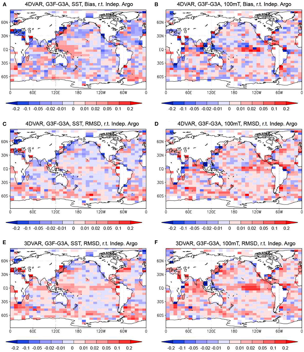
Figure 8. Difference of the bias absolute values and the RMSDs relative to the independent Argo float data between the MOVE-G3A and MOVE-G3F temperature in the 4DVAR and 3DVAR Runs. (A, B) Difference of the bias absolute values at the surface and 100 m depth in the 4DVAR Run. (C, D) Difference of the RMSDs at the surface and 100 m depth in the 4DVAR Run. (E, F) Same as (C, D) but for the 3DVAR Run. Blue colors mean that the bias absolute value or the RMSD is smaller for the MOVE-G3F temperature. Units in °C.

The differences of the RMSDs before and after the downscaling are also depicted for the 3DVAR Run in Figures 8E, F. These figures indicate that the increase in RMSD in the tropical regions and around the Kuroshio and the Gulf Stream at the surface and 100 m depth due to the downscaling is larger for the 3DVAR Run. The less increase in RMSD due to downscaling in the 4DVAR Run is presumably due to better physical balance of the MOVE-G3A field than in the 3DVAR Run.

As a result, the degradation of the MOVE-G3A temperature fields evaluated with the RMSD relative to independent Argo float data that occurs when introducing the 4DVAR Method is mitigated after downscaling. As for SST, although the RMSD of the MOVE-G3A field is generally larger for the 4DVAR Run (Figure 6A), the RMSD of the MOVE-G3F field in the western and eastern tropical Pacific, tropical Atlantic, eastern tropical Indian Ocean, western North Pacific and near the east coast of US and the Argentine coast is reduced compared to the 3DVAR Run (Figure 9C). In addition, the reduction of the RMSD of temperature at the 100 m depth by the 4DVAR method is enhanced after the downscaling in the central equatorial Pacific and Kuroshio extension area and along the Gulf Stream although the RMSD still increases in the 4DVAR Run over a wider area of the ocean even after the downscaling (Figure 7D). It should be noted that the 4DVAR Run reproduces a larger variance of temperature at the surface and 100 m depth compared with the 3DVAR Run in the most area even after the downscaling (Figures 9E, F). Although the larger variance tends to increase the RMSD, the RMSD is nevertheless smaller for the 4DVAR Run in several locations, including the western tropical and North Pacific surface layer and the central tropical Pacific at 100 m depth.

FIGURE 9

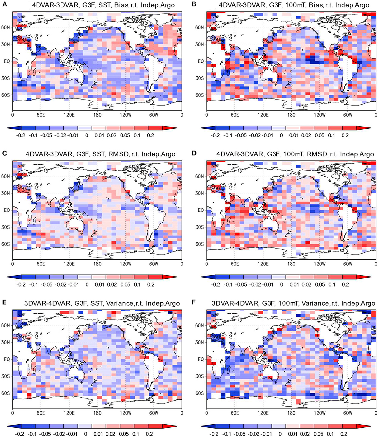
Figure 9. Difference of the bias absolute values, RMSDs, and relative standard deviations of the MOVE-G3F temperature relative to the independent Argo float data between the 4DVAR and 3DVAR Runs. (A, B) Difference of the bias absolute values at the surface and 100 m depth. (C, D) Difference of the RMSDs at the surface and the 100 m depth. (E, F) Difference of the relative standard deviations at the surface and the 100 m depth. Blue colors mean that the bias absolute value and the RMSD are smaller for the 4DVAR Run in (A–D), and that the relative standar deviation is larger for the 4DVAR Run in (E, F). Units in °C.

In addition, the 4DVAR method reduces the SST bias relative to the independent Argo float data in most areas except the North Atlantic before the downscaling, and the reduction is maintained after the downscaling (Figure 9A). The areas of decreasing the bias of the MOVE-G3F temperature at 100 m depth in the 4DVAR Run is also pronounced than the areas of increasing the bias (Figure 9B), as it is before the downscaling (not shown).

Distributions of the bias and the RMSD of the MOVE-G3F temperature relative to the independent Argo float data in the equatorial vertical section for the 4DVAR Run are shown along with the bias absolute value and the RMSD differences between the 4DVAR Run and 3DVAR Runs in Figures 10A–D. Relatively large bias and RMSD can be seen along the thermocline in the 4DVAR Run. There are extremely large negative bias (down to −3.5°C) and RMSD (up to 4.7°C) at the eastern edge of the Pacific, possibly due to insufficient representation of the Galapagos Islands and coastal upwelling. Another large negative bias (down to −1.0°C) and RMSD (up to 2.9°C) are seen at the western edge of the Atlantic. Except for those locations, the largest bias (0.8°C) exists at the thermocline in the central equatorial Pacific and the RMSD is no larger than 2.4°C.

FIGURE 10

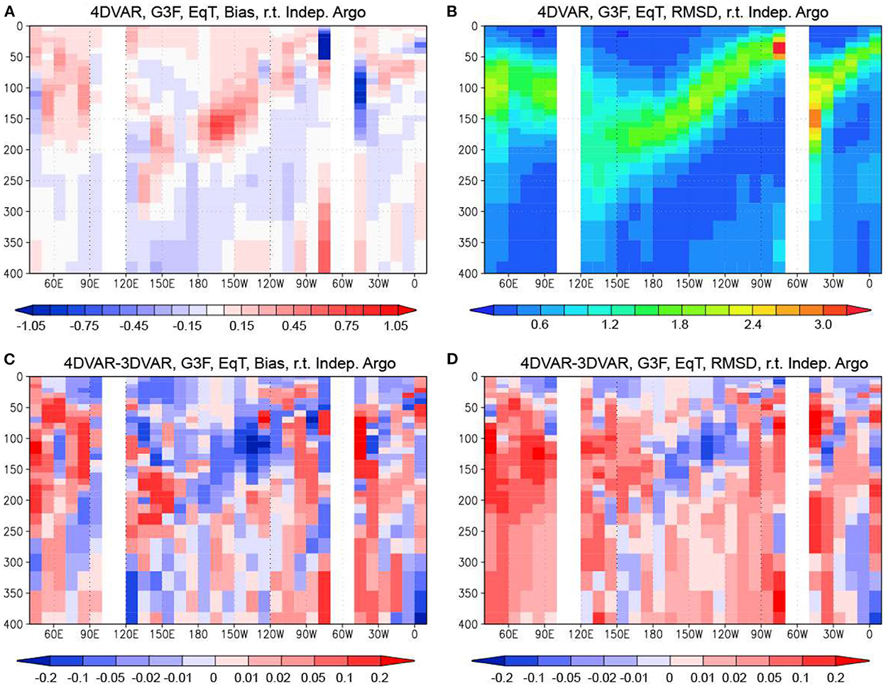
Figure 10. (A, B) Bias and RMSD of the MOVE-G3F temperature at the equatorial vertical section (average of two boxes within 5°S−5°N) in the 4DVAR Run. 3DVAR Run Difference of the bias absolute values and RMSDs of the MOVE-G3F temperature between the 4DVAR and 3DVAR Runs at the equatorial vertical section. The biases and RMSDs are relative to the independent Argo float data. Blue colors in (C, D) mean that the bias absolute value or the RMSD is smaller for the 4DVAR Run. Units in °C.

Then, the difference of the bias absolute values indicates that the 4DVAR method reduces the bias at relatively many locations such as near surface and around the thermocline. The RMSD is also reduced around the thermocline in the equatorial Pacific, as well as in the near surface layer. The reduction of the bias and the RMSD around the thermocline by introducing the 4DVAR method is expected to have a positive impact on ENSO forecasts.

5. Summary and discussion

This paper first described the ocean models and the data assimilation and downscaling methods employed in the JMA's new global ocean data assimilation system for the coupled predictions, MOVE/MRI.COM-G3. The system is composed of the lower-resolution subsystem, MOVE-G3A, and the higher-resolution subsystem, MOVE-G3F. MOVE-G3A has zonal and meridional resolutions of 1.0° and 0.5°, and adopts a 4DVAR method with a 10-day data assimilation window to optimize the increments added to the temperature and salinity fields of the ocean model within the first 5 days using observation data within the second 5 days. Then, the data-assimilated temperature and salinity fields in MOVE-G3A are downscaled into MOVE-G3F with a resolution of 0.25° through IAU.

Then, the impact of introducing the 4DVAR method was investigated through the comparison of a regular reanalysis run of MOVE/MRI.COM-G3 (4DVAR Run) with a reanalysis run using a 3DVAR method instead of the 4DVAR method (3DVAR Run). Before the downscaling, the bias and RMSD of SST and 100-m-depth temperature relative to the assimilated data (MGDSST and the assimilated Argo float data) at the surface and 100 m depth were smaller in most parts of the ocean for the 4DVAR Run, which indicates that the 4DVAR method can more effectively reduce the misfits between the model field and observation data. This result is consistent with the former study of Weaver et al. (2003). However, when the independent Argo float data are used as the reference, the RMSDs of the SST and 100 m depth temperature increased in more than half of the areas in the 4DVAR Run. An increase in the variance of the temperature in the 4DVAR Run implies that the 4DVAR method adjusts the temperature fields more significantly but the adjustments are inconsistent with the independent observation data due to insufficient model physics and resolution.

The downscaling to MOVE-G3F generally reduced the SST RMSD relative to the independent Argo float data except in the equatorial Pacific and the Southern Ocean, but generally increases the RMSD of temperature at 100 m depth, in the 4DVAR Run. However, the area in which the SST RMSD are reduced by the downscaling was shrunk and the increase of the RMSD for SST and 100-m-depth temperature was even greater in the 3DVAR Run. As a result, the increase in the RMSD relative to the independent Argo float data by introducing the 4DVAR method was mitigated after the downscaling. The RMSD was reduced for the 4DVAR Run in the western and eastern tropical Pacific and the western North Pacific for SST, and in the central equatorial Pacific and Kuroshio extension area for 100-m-depth temperature. The introduction of the 4DVAR method also reduced the bias absolute value and RMSD of temperature relative to the independent Argo float data along the thermocline as well as near surface in the equatorial vertical section.

However, it should be noted here that the improvement with 4DVAR is a trade-off for the extra time that 4DVAR takes over 3DVAR. On the one hand, the 3DVAR method of MOVE-G3A requires to perform 5-day integration of the lower-resolution model twice to obtain the analysis fields for 5 days. On the other hand, the 4DVAR method requires about 20 iterations of 10-day integrations of the lower-resolution model and its adjoint model to obtain the analysis fields for 5 days, which takes 60 times longer than the 3DVAR method since the integration time of the adjoint model takes about twice as long as the integration of the original model. To downscale to a higher-resolution system using either method, the higher-resolution model must be integrated for a total of 10 days. Since the integration time for the higher-resolution model is about 16 times longer than for the lower-resolution model, the computation time for the 4DVAR, including downscaling, is about 4.5 times longer than for the 3DVAR.

It should be also noted that the 4DVAR method estimates the analysis increments for a 5-day period using the data observed during the following 5 days, but the 3DVAR method estimates the increments for a 5-day period using the data obseved in the same period. One might consider that the cause of increasing the RMSD of temperature relative to the independent Argo data in the 4DVAR Run is the shift of the observation window from the period for which analysis increments are estimated. Therefore, in order to examine the effect of shifting the observation window, we conducted a supplemental reanalysis run (named the NS4DV Run) in which the analysis increments for the 5-day analysis window are estimated by the 4DVAR method using the data observed within the same window through the 4DVAR method.

Figure 11 shows the differences of RMSDs of the MOVE-G3A temperature relative to the independent Argo float data between the 4DVAR and NS4DV Runs at the surface and 100 m depth. This figure indicates that the RMSD is smaller for the 4DVAR Run in most areas except at the surface and 100 m depth in the Arctic Ocean and near the Antarctic coast, and at 100 m depth in the western tropical Indian Ocean. The temperature field is, thus, generally improved by the shift of the observation window in the 4DVAR Run because the longer integration of the adjoint model allows the information of observation data to propagate over a wider area and systematic model errors do not significantly affect the propagation.

FIGURE 11

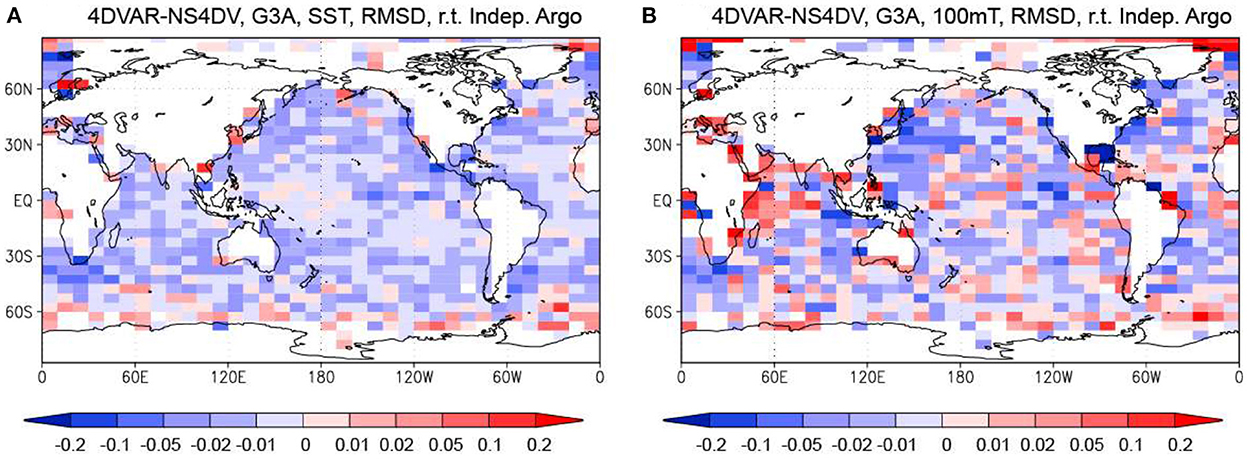
Figure 11. Difference of RMSDs of the MOVE-G3A temperature relative to the independent Argo float data between the 4DVAR and NS4DV Runs. (A) Difference of the RMSD at the surface. (B) Difference of the RMSDs at 100 m depth. Blue colors mean that the RMSD are smaller for the 4DVAR Run. Units in °C.

Another possible reason for the smaller RMSD of temperature in the 3DVAR Run is that the observation data within the 5-day observation window were dense enough that the benefit of using the adjoint model in the 4DVAR Run was reduced. However, if a shorter observation window is adopted, it may not be possible to obtain sufficiently dense observation data from that window, and the benefits of the 4DVAR method become more significant. Therefore, we also conduct two other supplementary reanalysis runs, the SW4DV and SW3DV Runs: in the SW4DV Run, analysis increments for a given day are optimized using data observed on the next day by the 4DVAR method; in the SW3DV Run, analysis increments for a given day are estimated from the data observed on the day by the 3DVAR method. The statistical parameters for data assimilation are not changed.

Figures 12A, B indicate that the RMSD of temperature relative to the independent Argo float data before the downscaling is generally larger when the shorter data assimilation window is adopted. In the SW4DV Run, the RMSD decreases for SST in the narrow areas around the western boundary currents, where frequent estimates of analysis increments seem to be effective because the lower resolution model has large systematic errors. However, the SST RMSD is increasing in most other areas. As for the 100 m depth, the RMSD is significantly increasing along the equator. Then, Figures 12C, D compares the RMSDs between SW4DV and SW3DV Runs. The SW4DV Run has a smaller RMSD of SST in most areas except in the tropical Indian Ocean, and western tropical Pacific. As for 100 m depth, although the RMSD is larger for the SW4DV Run in the tropical Pacific, tropical Indian Ocean, along the Antarctic coast, and in the Arctic Ocean, but is smaller in other areas. In particular, RMSD is significantly reduced in the areas around the western boundary currents. Thus, the 4DVAR method generally reduces the temperature RMSD except at 100 m depth in the tropical Pacific and tropical Atlantic Ocean, and the benefit of the 4DVAR method, therefore, increases when the daily assimilation window is applied. In fact, the daily assimilation window may be applied to the operatioal system in the future since it is easier to provide daily analysis fields, and if this were to happen, the advantage of the 4DVAR method would appear more clearly.

FIGURE 12

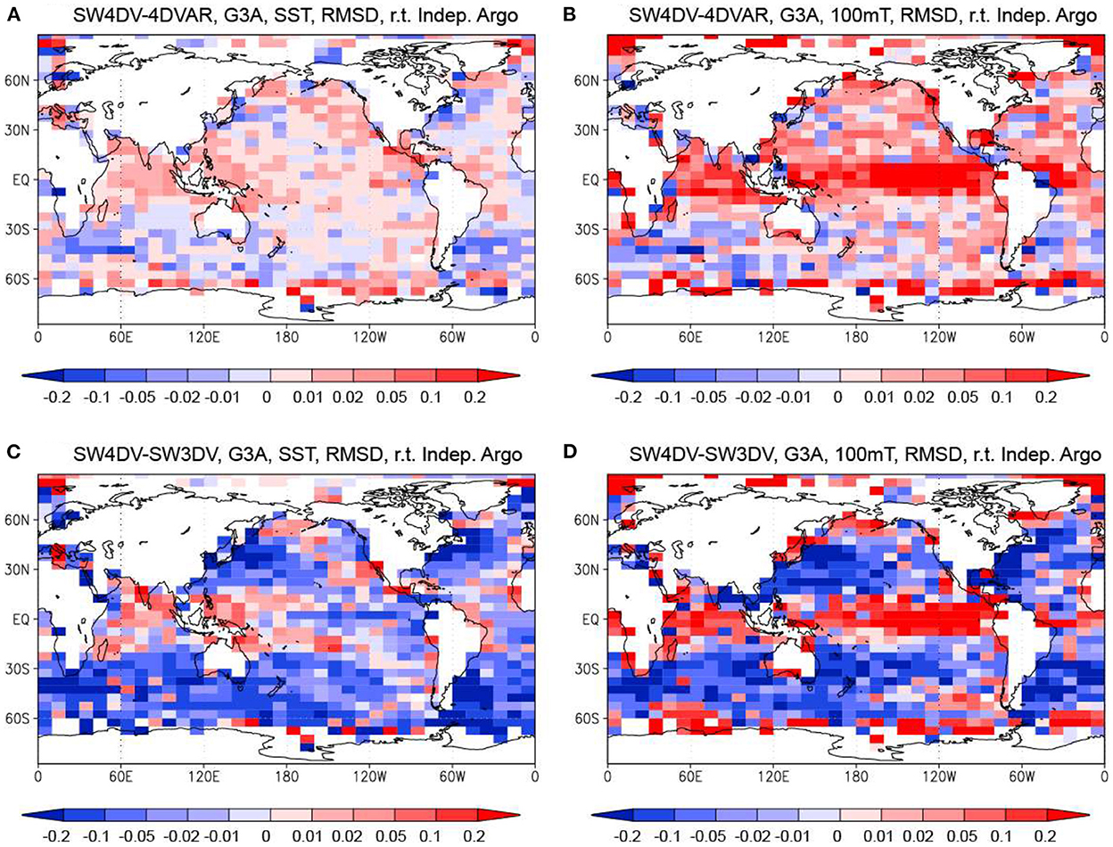
Figure 12. Difference of RMSDs of the MOVE-G3A temperature relative to the independent Argo float data between the SW4DV and 4DVAR Runs (A, B) and between the SW4DV and SW3DV Runs (C, D). (A, C) Difference of the RMSD at the surface. (B, D) Difference of the RMSDs at 100 m depth. Blue colors mean that the RMSD are smaller for the SW4DV Run. Units in °C.

The insufficient resolution of the ocean model used for the 4DVAR method is another highly potential reason why the advantages of the 4DVAR method are not clearly visible. Using a higher-resolution adjoint model, we can more accurately propagate the information of the observation data, and adjust the model fields in a manner more consistent with the independent observation data. Therefore, we plan to develop the next-generation global ocean data assimilation system using the 4DVAR method with higher-resolution forward and adjoint ocean models.

Data availability statement

The raw data supporting the conclusions of this article will be made available by the authors, without undue reservation.

Author contributions

YF and TY composed the ocean data assimilation system MOVE/MRI.COM-G3 and conducted the reanalysis runs used in this work. SU provided the one ocean model for MOVE-G3A, while HS and II provided the other ocean model for MOVE-G3F. YF made the analysis and drafted the manuscript with the support of other authors. All authors approved the submitted version.

Acknowledgments

The authors thank those who participated in the development of the ocean models and data assimilation schemes, including Goro Yamanaka, Hiroyuki Tsujno, Hideyuki Nakano, Takahiro Toyoda, Kei Sakamoto, Norihisa Usui, and Nariaki Hirose. The calculations for this work were performed on the FUJITSU Sever PRIMERGY CX2550 M5 super computer system of JMA/MRI.

Conflict of interest

The authors declare that the research was conducted in the absence of any commercial or financial relationships that could be construed as a potential conflict of interest.

Publisher's note

All claims expressed in this article are solely those of the authors and do not necessarily represent those of their affiliated organizations, or those of the publisher, the editors and the reviewers. Any product that may be evaluated in this article, or claim that may be made by its manufacturer, is not guaranteed or endorsed by the publisher.

References

Adcroft, A., and Campin, J.-M. (2004). Rescaled height coordinates for accurate representation of free-surface flows in ocean circulation models. Ocean Modell. 7, 269–284. doi: 10.1016/j.ocemod.2003.09.003

CrossRef Full Text | Google Scholar

AVISO (2015). “MSLA and (M)ADT near-real time and delayed time products,” in CLS-DOS-NT-06-034, Issue 4.4, Date:2015/06/30, Nomenclature: SALP-MU-P-EA-21065-CLS (Ramonville St-Agne: Collecte Localisation Satellites (CLS)).

Balmaseda, M. A., Dee, D., Vialard, A., and Anderson, D. T. L. (2007). A multivariate treatment of bias for sequential data assimilation: application to the tropical oceans. Q. J. R. Meteorol. Soc. 133, 167–179. doi: 10.1002/qj.12

CrossRef Full Text | Google Scholar

Bloom, S. C., Takas, L. L., Da Silva, A. M., and Ledvina, D. (1996). Data assimilation using incremental analysis updates. Mon. Weather. Rev. 124, 1256–1271.

Google Scholar

Boyer, T. P., Antonov, J. I., Baranova, O. K., Coleman, C., Garcia, H. E., Grodsky, A., et al. (2013). “World ocean database 2013,” in NOAA Atlas NESDIS (Silver Spring, MD: NOAA), Vol. 72, 209.

Google Scholar

Boyer, T. P., Baranova, O. K., Coleman, C., Garcia, H. E., Grodsky, A., Locarnini, R. A., et al. (2018). “World ocean database 2018,” in NOAA Atlas NESDIS, Vol. 87, ed A. V. Mishonov (Silver Spring, MD: NOAA), 207.

Google Scholar

Forget, G., Campin, J.-M., Heimbach, P., Hill, C. N., Ponte, R. M., and Wunsch, C. (2015). ECCO version 4: an integrated framework for non-linear inverse modeling and global ocean state estimation. Geosci. Model Dev. 8, 3071–3104. doi: 10.5194/gmd-8-3071-2015

CrossRef Full Text | Google Scholar

Fujii, Y. (2005). Preconditioned optimizing utility for large-dimensional analyses (POpULar). J. Oceanogr. 61, 167–181. doi: 10.1007/s10872-005-0029-z

CrossRef Full Text | Google Scholar

Fujii, Y., Ishizaki, S., and Kamachi, M. (2005). Application of nonlinear constraints in a three-dimensional variational ocean analysis. J. Oceanogr. 61, 655–662. doi: 10.1007/s10872-005-0073-8

CrossRef Full Text | Google Scholar

Fujii, Y., and Kamachi, M. (2003a). Three-dimensional analysis of temperature and salinity in the equatorial Pacific using a variational method with vertical coupled temperature-salinity empirical orthogonal function modes. J. Geophys. Res. 108, 3297. doi: 10.1029/2002JC001745

CrossRef Full Text | Google Scholar

Fujii, Y., and Kamachi, M. (2003b), A nonlinear preconditioned quasi-Newton method without inversion of a first-guess covariance matrix in variational analyses. Tellus 55A, 450–454. doi: 10.1034/j.1600-0870.2003.00030.x

CrossRef Full Text | Google Scholar

Fujii, Y., Nakaegawa, T., Matsumoto, S., Yasuda, T., Yamanaka, G., and Kamachi, M. (2009). Coupled climate simulation by constraining ocean fields in a coupled model with ocean data. J. Clim. 22, 5541–5557. doi: 10.1175/2009JCLI2814.1

CrossRef Full Text | Google Scholar

Fujii, Y., Ogawa, K., Brassington, G. B., Ando, K., Yasuda, T., and Kuragano, T. (2015). Evaluating the impacts of the tropical Pacific observing system on the ocean analysis fields in the global ocean data assimilation system for operational seasonal forecasts in JMA. J. Oper. Oceanogr. 8, 25–39. doi: 10.1080/1755876X.2015.1014640

CrossRef Full Text | Google Scholar

Fujii, Y., Tsujino, H., Usui, N., Nakano, H., and Kamachi, M. (2008). Application of singular vector analysis to the Kuroshio large meander. J. Geophys. Res. 113, C07026. doi: 10.1029/2007JC004476

CrossRef Full Text | Google Scholar

Gent, P. R., and McWilliams, J. C. (1990). Isopycnal mixing in ocean circulation models. J. Phys. Oeanogr. 20, 150–155. doi: 10.1175/1520-0485(1990)020<0150:IMIOCM>2.0.CO;2

PubMed Abstract | CrossRef Full Text | Google Scholar

Hackert, E., Kovach, R. M., Molod, A., Vernieres, G., Borovikov, A., Marshak, J., et al. (2020). Satellite sea surface salinity observations impact on El Niño/Southern Oscillation predictions: case studies from the NASA GEOS seasonal forecast system. J. Geophys. Res. 125, e2019JC015788. doi: 10.1029/2019JC015788

CrossRef Full Text | Google Scholar

Hamilton, D. (1994). GTSPP builds an ocean temperature-salinity database. Earth Syst. Monit. 4, 4–5.

Google Scholar

Hirahara, S., Kubo, Y., Yoshida, T., Komori, T., Chiba, J., Sekiguchi, R., et al. (in press). Japan meteorological agency/meteorological research institute-coupled prediction system version 3 (JMA/MRI-CPS3). J. Meteor. Soc. Jpn.

Google Scholar

Hirose, N., Usui, N., Sakamoto, K., Tsujino, H., Yamanaka, G., Nakano, H., et al. (2019). Development of a new operational system for monitoring and forecasting coastal and open ocean states around Japan. Ocean Dyn. 69, 1333–1357. doi: 10.1007/s10236-019-01306-x

CrossRef Full Text | Google Scholar

Huang, B., Liu, C., Banzon, V., Freeman, E., Graham, G., Hankins, B., et al. (2021). Improvements of the daily optimum interpolation sea surface temperature (DOISST) Version 2.1. J. Clim. 34, 2923–2939. doi: 10.1175/JCLI-D-20-0166.1

CrossRef Full Text

Hudson, D., Alves, O., Hendon, H. H., Lim, E.-P., Liu, G., Luo, J.-J., et al. (2017). ACCESS-S1 the new Bureau of meteorology multi-week to seasonal prediction system. J. South. Hemisphere Earth Syst. Sci. 67, 132–159. doi: 10.1071/ES17009

CrossRef Full Text | Google Scholar

Hunke, C. E., and Lipscomb, W. H. (2006). “CICE: the Los Alamos sea ice model documentation and software user's manual,” in Technical Report LA-CC-98-16, 59, T-3 Fluid Dynamics Group (Los Alamos, NM: Los Alamos National Laboratory), 87545–87559.

Google Scholar

JMA (2022). “Outline of the operational numerical weather prediction at the Japan Meteorological Agency,” in Appendix to WMO Technical Progress Report on the Global Data-Processing and Forecasting System and Numerical Weather Prediction (Tokyo: JMA).

Kobayashi, S., Kosaka, Y., Chiba, J., Tokuhiro, T., Harada, Y., Kobayashi, C., et al. (2021). “JRA-3Q: Japanese reanalysis for three quarters of a century,” in WCRP-WWRP Symposium on Data Assimilation and Reanalysis/ECMWF Annual Seminar 2021 (Geneva: WMO).

Köhl, A. (2015). Evaluation of the GECCO2 ocean synthesis: transports of volume, heat and freshwater in the Atlantic. Q. J. Roy. Metor. Soc. 141, 166–181. doi: 10.1002/qj.2347

CrossRef Full Text | Google Scholar

Kuragano, T., Fujii, Y., Toyoda, T., Usui, N., Ogawa, K., and Kamachi, M. (2014). Seasonal barotropic sea surface height fluctuation in relation to regional ocean mass variation. J. Oceanogr. 70, 45–62. doi: 10.1007/s10872-013-0211-7

CrossRef Full Text | Google Scholar

Kurihara, Y., Sakurai, T., and Kuragano, T. (2006). Global daily sea surface temperature analysis using data from satellite microwave radiometer, satellite infrared radiometer and in-situ observations. Weath. Bull. 73, s1–s18.

Google Scholar

Large, W. G., and Yeager, S. (2004). Diurnal to Decadal Global Forcing for Ocean and Sea-Ice Models: The Data Sets and Flux Climatologies. NCAR Technical Note TN-460+STR. Boulder, CO: NCAR. p. 105.

Google Scholar

Leonard, B. P. (1979). A stable and accurate convective modeling procedure based upon quadratic upstream interpolation. J. Comput. Methods Appl. Mech. Eng. 19, 59–98. doi: 10.1016/0045-7825(79)90034-3

CrossRef Full Text | Google Scholar

Locarnini, R. A., Mishonov, A. V., Baranova, O. K., Boyer, T. P., Zweng, M. M., Garcia, H. E., et al. (2019). “World Ocean Atlas 2018. Volume 1: temperature,” in Technical Editor. NOAA atlas NESDIS, ed A. Misonov (Silver Spring, MD: NOAA), 52.

Matsumoto, T., Ishii, M., Fukuda, Y., and Hirahara, S. (2006). “Sea ice data derived from microwave radiometer for climate monitoring,” in Proceedings of the 14th Conference on Satellite Meteorology and Oceanography (Washington, DC: American Meteorological Society).

Google Scholar

Mazloff, M. R., Heimbach, P., and Wunsch, C. (2010). An eddy-permitting southern ocean state estimate. J. Phys. Oceangr. 40, 880–899. doi: 10.1175/2009JPO4236.1

CrossRef Full Text | Google Scholar

Mellor, G. L., and Kantha, L. (1989). An ice-ocean coupled model. J. Geophys. Res. 94, 10937–10954.

Google Scholar

Mochizuki, T., Masuda, S., Ishikawa, Y., and Awaji, T. (2016). Multiyear climate prediction with initialization based on 4D-Var data assimilation. Geophys. Res. Lett. 43, 3903–3910. doi: 10.1002/2016GL067895

CrossRef Full Text | Google Scholar

Moore, M. A., Arango, H. G., Broquet, G., Powell, B. S., Weaver, A. T., and Zavala-Garay, J. (2011). The regional ocean modeling system (ROMS) 4-dimensional variational data assimilation systems: Part I—system overview and formulation. Prog. Oceangr. 91, 34–49. doi: 10.1016/j.pocean.2011.05.004

CrossRef Full Text | Google Scholar

Murray, R. J. (1996). Explicit generation of orthogonal grids for ocean models. J. Comput. Phys. 126, 251–273. doi: 10.1006/jcph.1996.0136

CrossRef Full Text | Google Scholar

Nakano, H., and Suginohara, N. (2002). Effects of bottom boundary layer parameterization on reproducing deep and bottom waters in a world ocean model. J. Phys. Oceanogr. 32, 1209–1227. doi: 10.1175/1520-0485(2002)032<1209:EOBBLP>2.0.CO;2

CrossRef Full Text | Google Scholar

Osafune, S., Masuda, S., Sugiura, N., and Doi, T. (2015). Evaluation of the applicability of the Estimated Ocean State for Climate Research (ESTOC) dataset. Geophys. Res. Lett. 42, 4903–4911. doi: 10.1002/2015GL064538

CrossRef Full Text | Google Scholar

Pohlmann, H., Jungclaus, J. H., Köhl, A., Stammer, D., and Marotzke, J. (2009). Initializing decadal climate predictions with the GECCO oceanic synthesis: effects on the North Atlantic. J. Clim. 22, 3926–3938. doi: 10.1175/2009JCLI2535.1

CrossRef Full Text | Google Scholar

Prather (1986). Numerical advection by conservation of second-order moments. J. Geophys. Res. 91, 6671–6681. doi: 10.1029/JD091iD06p06671

CrossRef Full Text | Google Scholar

Redi, M. H. (1982). Oceanic isopycnal mixing by coordinate rotation. J. Phys. Oceanogr. 12, 1154–1158. doi: 10.1175/1520-0485(1982)012<1154:OIMBCR>2.0.CO;2

CrossRef Full Text | Google Scholar

Sugiura, N., Awaji, T., Masuda, S., Mochizuki, T., Toyoda, T., Miyama, T., et al. (2008). Development of a four-dimensional variational coupled data assimilation system for enhanced analysis and prediction of seasonal to interannual climate variations. J. Geophys. Res. 113, C10017. doi: 10.1029/2008JC004741

CrossRef Full Text | Google Scholar

Toyoda, T., Fujii, Y., Yasuda, T., Usui, N., Ogawa, K., Kuragano, T., et al. (2016). Data assimilation of sea ice concentration into a global ocean–sea ice model with corrections for atmospheric forcing and ocean temperature fields. J. Oceanogr. 72, 235–262. doi: 10.1007/s10872-015-0326-0

CrossRef Full Text | Google Scholar

Tsujino, H., Nakano, H., Sakamoto, K., Urakawa, S., Hirabara, M., Ishizaki, H., et al. (2017). Reference manual for the meteorological research institute community ocean model version 4 (MRI.COMv4). Tech. Rep. Meteorol. Res. Inst. Jpn. 80, 306. doi: 10.11483/mritechrepo.80

CrossRef Full Text

Umlauf, L., and Burchard, H. (2003). A generic length-scale equation for geophysical turbulence models. J. Mar. Res. 61, 235–265. doi: 10.1357/002224003322005087

CrossRef Full Text | Google Scholar

Usui, N., Fujii, Y., Sakamoto, K., and Kamachi, M. (2015). Development of a four-dimensional variational assimilation system toward coastal data assimilation around Japan. Mon. Wea. Rev. 143, 3874–3892. doi: 10.1175/MWR-D-14-00326.1

CrossRef Full Text | Google Scholar

Usui, N., Ishizaki, S., Fujii, Y., and Kamachi, M. (2011). Improving strategies with constraints regarding non-Gaussian statistics in a three-dimensional variational assimilation method. J. Oceanogr. 67, 253–262. doi: 10.1007/s10872-011-0024-5

CrossRef Full Text | Google Scholar

Vialard, J., Weaver, A. T., Anderson, D. L. T., and Delecluse, P. (2003). Three- and four-dimensional variational assimilation with a general circulation model of the tropical Pacific Ocean. Part II: physical validation. Mon. Wea. Rev. 131, 1379–1395. doi: 10.1175/1520-0493(2003)131<1379:TAFVAW>2.0.CO;2

CrossRef Full Text | Google Scholar

Visbeck, M., Marshall, J., Haine, T., and Spall, M. (1997). Specification of eddy transfer coefficients in coarse-resolution ocean circulation models. J. Phys. Oceanogr. 27, 381–402. doi: 10.1175/1520-0485(1997)027<0381:SOETCI>2.0.CO;2

CrossRef Full Text | Google Scholar

Waters, J., Lea, D., Martin, M., Mirouze, I., Weaver, A., and While, J. (2015). Implementing a variational data assimilation system in an operational 1/4 degree global ocean model. Q. J. Roy. Meteor. Soc. 141, 333–349. doi: 10.1002/qj.2388

CrossRef Full Text | Google Scholar

Weaver, A. T., Deltel, C., Machu, E., Ricci, S., and Daget, N. (2005). A multivariate balance operator for variational ocean data assimilation. Q. J. Roy. Meteor. Soc. 131, 3605–3625. doi: 10.1256/qj.05.119

CrossRef Full Text | Google Scholar

Weaver, A. T., Vialard, J., and Anderson, D. L. T. (2003). Three- and four-dimensional variational assimilation with a general circulation model of the tropical pacific ocean. Part I: formulation, internal diagnostics, and consistency checks. Mon. Wea. Rev. 131, 1360–1378. doi: 10.1175/1520-0493(2003)131<1360:TAFVAW>2.0.CO;2

CrossRef Full Text | Google Scholar

Xue, Y., Huang, B., Hu, Z.-Z., Kumar, A., Wen, C., Behringer, D., and Nadiga, S. (2011). An assessment of oceanic variability in the NCEP climate forecast system reanalysis. Clim. Dyn. 37, 2511–2539. doi: 10.1007/s00382-010-0954-4

CrossRef Full Text | Google Scholar

Zuo, H., Balmaseda, M. A., Tietsche, S., Mogensen, K., and Mayer, M. (2019). The ECMWF operational ensemble reanalysis–analysis system for ocean and sea ice: a description of the system and assessment. Ocean Sci. 15, 779–808. doi: 10.5194/os-15-779-2019

CrossRef Full Text | Google Scholar

Zweng, M. M., Reagan, J. R., Seidov, D., Boyer, T. P., Locarnini, R. A., Garcia, H. E., et al. (2019). “World ocean atlas 2018. volume 2: salinity,” in Technical Editor, NOAA Atlas NESDIS, ed A. Mishonov (Silver Spring, MD: NOAA), 50.

Google Scholar