 Abayomi A. Abatan
 Matthew Collins
 Mukand S. Babel
 Dibesh Khadka
 Yenushi K. De Silva
95% of researchers rate our articles as excellent or good
Learn more about the work of our research integrity team to safeguard the quality of each article we publish.
Find out more
ORIGINAL RESEARCH article
Front. Clim. , 05 October 2021
Sec. Climate Services
Volume 3 - 2021 | https://doi.org/10.3389/fclim.2021.716129
The boreal summer intraseasonal oscillation (BSISO) plays an important role in the intraseasonal variability of a wide range of weather and climate phenomena across the region modulated by the Asian summer monsoon system. This study evaluates the strengths and weaknesses of 19 Coupled Model Intercomparison Project Phase 6 (CMIP6) models to reproduce the basic characteristics of BSISO. The models' rainfall and largescale climates are evaluated against GPCP and ERA5 reanalysis datasets. All models exhibit intraseasonal variance of 30–60-day bandpass-filtered rainfall and convection anomalies but with diverse magnitude when compared with observations. The CMIP6 models capture the structure of the eastward/northward propagating BSISO at wavenumbers 1 and 2 but struggle with the intensity and location of the convection signal. Nevertheless, the models show a good ability to simulate the power spectrum and coherence squared of the principal components of the combined empirical orthogonal function (CEOF) and can capture the distinction between the CEOF modes and red noise. Also, the result shows that some CMIP6 models can capture the coherent intraseasonal propagating features of the BSISO as indicated by the Hovmöller diagram. The contribution of latent static energy to the relationship between the moist static energy and intraseasonal rainfall over Southeast Asia is also simulated by the selected models, albeit the signals are weak. Taking together, some of the CMIP6 models can represent the summertime climate and intraseasonal variability over the study region, and can also simulate the propagating features of BSISO, but biases still exist.
In boreal winter, the Madden-Julian Oscillation (MJO; Madden and Julian, 1972, 1994) is the dominant mode of tropical intraseasonal variability while boreal summer is dominated by intraseasonal oscillation (e.g., Yasunari, 1979; Lee et al., 2013; Li and Mao, 2019). These oscillations are characterized by eastward- and northward-propagation across the tropics and have a significant effect on global weather and climate at different timescales (Straub and Kiladis, 2003; Lin et al., 2006; Kim et al., 2009; Ahn et al., 2017; and references therein). However, the characteristic features (e.g., propagation, intensity, etc.) of the boreal summer intraseasonal oscillation (BSISO) is more complex than that of MJO (Annamalai and Sperber, 2005; Lee et al., 2013; Li and Mao, 2016; Qi et al., 2019; and references therein). For example, MJO is a dominant eastward propagating mode along the equator with a 20–100-day oscillation across the globe (e.g., Duffy et al., 2003; Inness and Slingo, 2003; Waliser et al., 2003a; Jones et al., 2004; Zhang et al., 2006; Kim et al., 2009; Alaka and Maloney, 2012; Yoneyama et al., 2013; Eyring et al., 2016a; Ahn et al., 2017; Ling et al., 2019; Yang and Wang, 2019). BSISO, on the other hand, has two dominant time scales, 10–20-day and 30–60-day. The 10–20-day BSISO is characterized by westward propagation over the Indian summer monsoon region and northwestward propagation over the East Asia/western North Pacific region. The 30–60-day BSISO, however, is characterized by northward/northeastward propagation along the equatorial Indian Ocean and northward/northwestward propagation over the western North Pacific region (e.g., Mao and Chan, 2005; Wang et al., 2005; Kikuchi and Wang, 2010; Li and Mao, 2019). The BSISO is an important variability of the Asian summer monsoon system and it is associated with fluctuations in the onset and break of monsoons, droughts and floods, tropical cyclone activity, and remote teleconnections including the El Niño Southern Oscillation (Higgins and Shi, 2001; Waliser et al., 2003b; Lin and Li, 2008; Ko and Hsu, 2009; Hsu and Li, 2011; Li et al., 2015). In this regard, the intraseasonal variability and life cycle of the BSISO can cause discomfort to the inhabitants of the region; warranting a detailed understanding of the BSISO. Knowledge of the impact of the BSISO on the weather at a regional-scale, which is often rendered by the state-of-the-art General Circulation Models (GCMs), could provide useful information for weather-dependent operational decision making. Hence, it is important to assess the ability of climate models to simulate the characteristic features of BSISO.
A body of literature exists on the studies of BSISO simulation (e.g., Waliser et al., 2003b; Li and Mao, 2016; Hu et al., 2017; Yang et al., 2020). In general, most climate models continue to underestimate the intraseasonal variability of the BSISO and associated monsoon variability. The shortcomings are attributed to an inadequate understanding of BSISO mechanisms and an inaccurate representation of the parameterized physical processes, for example, cumulus convection, that are associated with BSISO simulation in the climate models (Waliser et al., 2003b; Hu et al., 2017; Qi et al., 2019). Using the Chinese Academy of Meteorological Sciences coupled climate science model (CAMS-CSM), Qi et al. (2019) evaluated the fidelity of this model to capture some basic features of BSISO. They showed that CAMS-CSM can reproduce the features of BSISO, but underestimated the zonal and meridional propagation over the Asian summer monsoon domain. This suggests that the model failed to adequately represent the BSISO convection. The role of vertical wind shear in the development of northward propagating BSISO has also been confirmed in previous studies (Inness et al., 2003; Jiang et al., 2004; Yang et al., 2019). This is further illustrated by Yang et al. (2019) in a series of NESM3.0 model experiments through lowering the Tibetan Plateau. The results showed that lowering Tibetan Plateau reduced the vertical wind shear, which in turn limited the BSISO northward propagation. This echoes the result of Qi et al. (2019) and demonstrates that accurate northward propagating BSISO is related to state-of-the-art climate models' ability to simulate the physical processes of the vertical structure of BSISO.
Assessment of the low frequency tropical intraseasonal oscillations (e.g., MJO and BSISO) and associated Asian summer monsoon variability in climate models that have participated in the Coupled Model Intercomparison Project (CMIP) appears in several previous studies (e.g., Lin et al., 2006, 2008; Sperber and Kim, 2012; Hung et al., 2013; Jena et al., 2016; Ahn et al., 2017; Preethi et al., 2019; Konda and Vissa, 2021). Evidence still abounds that many GCMs fall short at representing the basic features of these oscillations, including the northward propagating convection, because of resolution-sensitivity to parameterizations, large-scale dynamics, and representation of physical processes that vary from model to model (Sabeerali et al., 2013; Konda and Vissa, 2021). However, there has been a notable improvement in the robust simulation of intraseasonal variability from CMIP3 to CMIP5, due in part to increases in resolution and convective parameterization. Comparing the simulated BSISO eastward propagating convective anomalies in CMIP5 with those of the CMIP3, Sabeerali et al. (2013) noted a modest improvement in BSISO simulation in CMIP5 models. Ogata et al. (2014) applied Taylor's skill metrics to assess the performance of 20 CMIP3 and 24 CMIP5 models at capturing the seasonal mean structures of the summer Asian monsoon and reported an improvement in the skills of the CMIP5 multi-model ensemble mean. This result echoed the findings of Sperber et al. (2013) that CMIP5 models have good skill at reproducing the northward propagation of convection. Despite this improvement, simulation of the low frequency tropical intraseasonal oscillations remains a challenge (Konda and Vissa, 2021; Yan et al., 2021).
A considerable amount of effort by modeling groups has been devoted to improving their climate models. On average, the CMIP5 models have higher horizontal resolutions than those in CMIP3 and have improved subgrid-scale parameterizations than those used in the CMIP3 version (Hung et al., 2013). CMIP6 models are the newly released version of the CMIP family with improvement in resolution and physical complexity relative to other CMIPs (Taylor et al., 2012). Hence it is important to evaluate how well the CMIP6 climate models perform. A more recent study by Ahn et al. (2020) examined how well the CMIP6 models perform in simulating MJO propagation in comparison with CMIP5, with a focus on the Maritime Continent during boreal winter (November–April). This study concluded that MJO propagation is significantly improved in CMIP6 models compared to CMIP5 models. Several other studies have evaluated the performance of CMIP6 models to simulate the mean climate at both the global and the regional scales (Pattnayak et al., 2017; Wu et al., 2019; Xin et al., 2020; Khadka et al., 2021). There was a strong agreement that CMIP6 models showed an overall improvement in the skill scores of the climate patterns compared with CMIP5 models. To the best of our knowledge, the CMIP6 models have not been applied to study the summer intraseasonal oscillation.
This study focuses only on the period of May–October when some regions of Southeast Asia, like Thailand, experience a significant wet period. The ultimate motivation is to assess changes in BSISO-rainfall connections in Southeast Asia under climate change. This study represents the first step and the impact of climate change will be reported in future publications. Hence, this first part of our work aims to examine how well a subset of CMIP6 models simulates the basic characteristic features of BSISO. The remainder of this paper is organized such that the selected 19 CMIP6 climate models, validation datasets, and the diagnostic methods are introduced in section Region, Dataset, and Methods. Results are presented in section Results and the conclusions appear in section Conclusions.
Southeast Asia is the sub-region of Asia that stretches from about 10°S to 20°N and 100°E to 140°E including Cambodia, Laos, Myanmar, Thailand, Vietnam, and parts of southern China. The region is bordered by the Indian subcontinent in the west, the Indian Ocean in the south, China in the north, and Australia in the southeast. The climate of Southeast Asia is predominantly tropical, with a monsoonal circulation system being the main driver of the seasonal rainfall pattern (McSweeney et al., 2015). This region is under the influence of the Southeastern Asian summer monsoon system, and it is characterized by longer wet seasons (between 120 to 160 days) in the Asian monsoon domain (Misra and DiNapoli, 2014). The rainy season over this region typically begins in May and subsides in October (Zeng and Lu, 2004).
The historical runs of the Coupled Model Intercomparison Project phase 6 (CMIP6; Eyring et al., 2016b) climate models are used for the analysis of the BSISO variability in this study. The selected 19 coupled general circulation models come from several institutions and are available at different latitude and longitude grid sizes on a daily timescale (Table 1). The first ensemble member of each of the 19 CMIP6 models is selected based on the availability and completeness of rainfall (Pr), sea surface temperature (SST), top of the atmosphere radiation (outgoing longwave radiation, OLR), and the atmospheric variables (zonal and meridional winds; U and V). Also, these models offer promising future simulation data to be used in future studies. The atmospheric variables are provided on 8 pressure levels (1,000, 850, 700, 500, 250, 100, 50, and 10 hPa).
Table 1. 19 selected CMIP6 climate models used for the analysis in this study.
The selected CMIP6 climate models are evaluated with an observational dataset as a reference state. The atmospheric datasets are obtained from the European Centre for Medium-Range Weather Forecasts Reanalysis v5 (ERA5; Hersbach et al., 2020). The daily dataset is obtained from the sub-daily dataset, which is available on a spatial resolution grid of 0.25° × 0.25° from 1979 to 2014. In addition to the ERA5 OLR dataset, a comparison OLR dataset is obtained from the National Oceanic Atmospheric Administration (NOAA) National Centers for Environmental Information website (www.ncdc.noaa.gov/cdr/atmospheric). The 1.0° × 1.0° daily mean OLR data is available from 1979 to 2014. The OLR is estimated from high-resolution infrared sounder radiance observations for all-sky conditions. Further details of this dataset can be found in Ellingson et al. (1989) and Lee et al. (2004). The global observed daily precipitation data is obtained from the Global Precipitation Climatology Project (GPCP) version 1.3 (Huffman et al., 2001). This product is a blend of rainfall observations from gauge stations and satellite retrievals. The GPCP used in this study is at a spatial resolution of 1.0° × 1.0° for the period 1997–2014.
All the datasets are regridded to the same 1.0° × 1.0° longitude and latitude horizontal resolution for comparison with models. We analyze data for the period 1997–2014 because the NOAA OLR has some missing data in 1982, 1985, and 1994, which is not acceptable in the algorithm for the computation of the power and cross-spectrum.
Several diagnostics tools and statistics have been developed and applied to evaluate the ability of the climate models in reproducing the spatio-temporal characteristics, intensity, zonal location, and propagation behavior of both winter and summer intraseasonal oscillations (e.g., Li and Mao, 2016; Hu et al., 2017; Qi et al., 2019). The chief among the diagnostics statistics includes the moist static energy that represents the intensity of BSISO during summer, wavenumber-frequency power spectrum, and the combined empirical orthogonal function (CEOF). These statistics are used in this study and have also appeared in several studies (for example, Jiang et al., 2004; Kim et al., 2009; Waliser et al., 2009; Sperber and Kim, 2012; Li, 2014; Li and Mao, 2016; Ahn et al., 2017; Fan et al., 2021; and references therein).
The column integrated moist static energy (MSE) has been employed in previous studies to study the eastward propagation of the MJO (Jiang, 2017; Wang et al., 2018). However, in this study, we use this thermodynamic variable to examine the propagation features of the BSISO. The vertically integrated MSE (m) can be expressed as: 〈m〉 = 〈cpT〉 + 〈gz〉 + 〈Lvq〉, where the angle brackets signify the mass-weighted vertical integral from 1,000-hPa to 500-hPa level, T is the temperature, z is the geopotential height, q is the specific humidity, cp is the specific heat at constant pressure, g is the gravitational acceleration, and Lv is the latent heat of vaporization. The first two terms on the right-hand side of the equation are termed the dry static energy (DSE) and the last term is the latent static energy (LSE).
The observed and simulated BSISO characteristic features in this study are assessed using the diagnostics developed by the U.S. CLIVAR MJO Working Group (MJOWG; Kim et al., 2009; Waliser et al., 2009). We obtain the BSISO index by modifying the MJO diagnostics script1. We compute the BSISO index by applying the combined empirical orthogonal function (CEOF) analysis to the daily averaged 30–60-day band-pass filtered OLR and U850 anomalies. The empirical orthogonal function is a multivariate statistical tool often used in climate studies to extract and study the characteristics of the dominant spatial modes of climate variability (from large datasets), as well as their temporal variability (aka, principal component). The CEOFs are obtained by computing the eigenvalues (modes) and eigenvectors (principal component) of the spatial covariance matrix of the combined anomaly fields. Note that the eigenvalues give a measure of the percentage variance explained by each mode and the principal components of each mode are obtained by projecting the eigenvectors unto the weighted combined anomalies. Further information can be obtained from North et al. (1982) and the NCAR Climate Data Guide website2. For the computation of the CEOFs and subsequent BSISO, we focus the analysis over the Asian summer monsoon region (10°S−40°N, 40°E−160°E) during summer (May to October) for the period 1997 to 2014; for consistency with BSISO literature (Lee et al., 2013; Yang et al., 2019). The band-pass filtered OLR and U850 anomalies are calculated by applying the bandpass Lanczos filtered weights to the data series and then remove the effect of the interannual variation by subtracting the climatological annual cycle. Next, we normalize the OLR and U850 anomalies by their respective area-averaged standard deviation after which the two anomaly datasets are combined and CEOF analysis is applied. Finally, the daily BSISO index and phase are obtained from the principal component – time series of the multivariate BSISO index denoted as CEOF1 (or PC1) and CEOF2 (or PC2) – of the first two leading modes of CEOFs. These first two leading modes are considered to represent the space-time evolution of the BSISO (Abhik et al., 2016). This BSISO amplitude is given as (PC12 + PC22)1/2 and the phase is given as arctan (PC1/PC2). The BSISO life cycle is divided into eight phases of equal angular extent. Given the BSISO amplitude and the phases, composites of the spatio-temporal structure of large-scale features associated with the BSISO life cycle that highlights the intraseasonal variability and the extent of the BSISO northward/eastward propagation can be determined.
To evaluate the spatio-temporal characteristics of the models to reproduce the band-pass filtered climate variables and other propagating features of the BSISO, we employ the usage of several statistical metrics. These metrics include pattern correlation coefficient (r), root mean square error (rmse), mean bias error (mbe), mean (m; normalized by GPCP), standard deviation, east-west ratio (E/W), and north-south ratio (N/S). These metrics are calculated as appropriate for the figures presented in this study.
Previous studies indicated that maps of intraseasonal variance offer an essential standpoint for climate model simulations of the BSISO. To assess the spatial pattern of intraseasonal variability, Figure 1 presents the intraseasonal variance of 30–60-day bandpass-filtered rainfall anomalies from GPCP, ERA5, and CMIP6 model simulations during the May–October season for the period 1997–2014. The GPCP data show weaker variance over the land region of Southeast Asia and a large part of the Maritime Continent (Figure 1a). However, a higher variance of rainfall anomalies (≥ 8 mm2 day−2) is located over the Indian Ocean, Bay of Bengal, the coastal regions of India and Myanmar, and the East China Sea. This intraseasonal signal signifies the direct impacts of BSISO characteristics on rainfall variability over those regions consistent with previous studies (Waliser et al., 2009; Hu et al., 2017; Qi et al., 2019). The structure of the intraseasonal variance of 30–60-day bandpass-filtered rainfall anomaly in ERA5 (r = 0.61; Figure 1b) is consistent with that of GPCP and previous reanalysis study (Kim et al., 2019). The difference between these two datasets lies in the magnitude of the rainfall over the regions mentioned above where ERA5 shows higher rainfall variance. This signifies the observational uncertainty, which may be related to the differences in the data processing. The 10% isoline of the rainfall variability accounted for by the BSISO mode (30–60-day) is indicated by the blue contour. The regions with maxima variance also exhibit a large percent variance of rainfall anomaly indicating that BSISO accounts for more than 10% of the intraseasonal rainfall variability over those regions. Meanwhile, the impact of BSISO on the climate of the Southeast region is smaller than 10% over the land region.
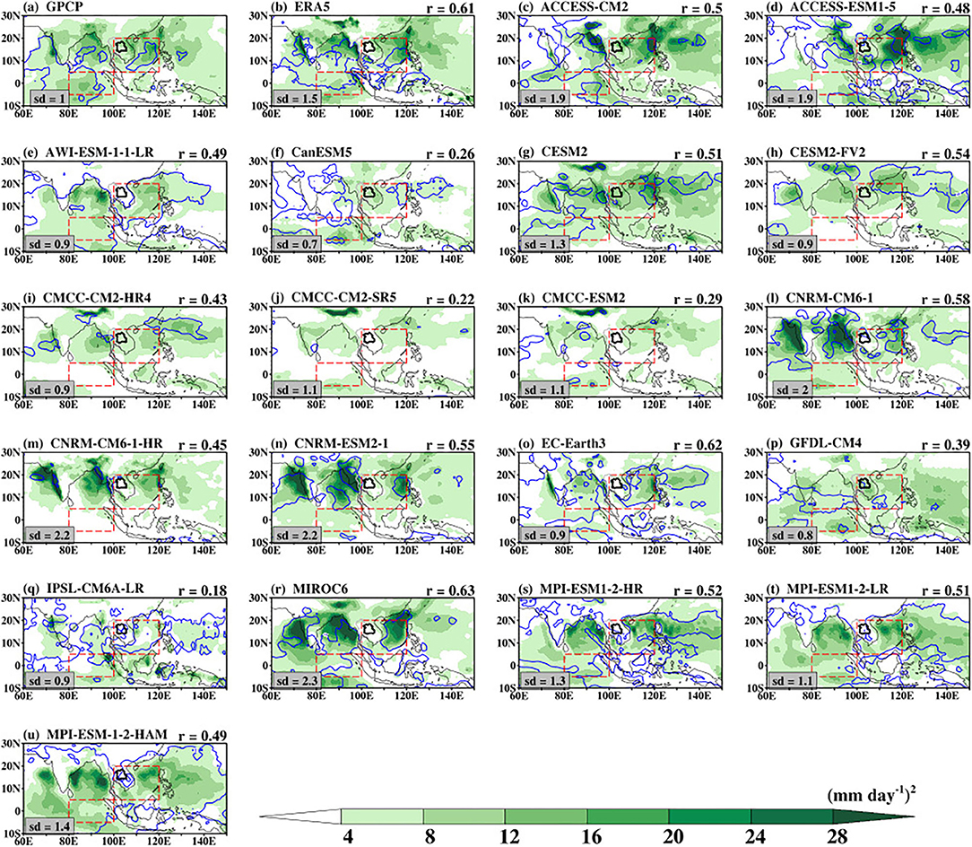
Figure 1. Variance of 30–60-day bandpass-filtered intraseasonal rainfall anomalies during the boreal summer (May–October) obtained from observations and CMIP6 models for the period 1997–2014. The Spearman correlation (r) of filtered rainfall anomaly on (b; ERA5) and (c–u; CMIP6 models) is obtained against (a) GPCP as the reference. The standard deviation of rainfall normalized by the GPCP standard deviation is shown at the bottom left of the plot. The blue contours represent the ratio of the 30–60-day bandpass-filtered intraseasonal rainfall variance to the total rainfall multiply by 100 (%). Only the 10% isoline of the rainfall variability is shown here. The dotted red boxes indicate the equatorial Indian Ocean and the Southeast Asia domain.
The CMIP6 climate models exhibit differences in the spatial structure and magnitude of the intraseasonal variance of 30–60-day bandpass-filtered rainfall anomalies as indicated by the statistical metrics in Table 2 and Figures 1c–u. For example, CanESM5 (Figure 1f), CMCC-CM2-SR5 (Figure 1j), CMCC-ESM2 (Figure 1k), GFDL-CM4 (Figure 1p), and IPSL-CM6A-LR (Figure 1q) show lower magnitude and thus missed the pattern of the observed rainfall variance as indicated by both the normalized mean (<0), rmse values (3.9 < rmse < 5.5 mm2 day−2) and weak pattern correlations (0.18 < r < 0.39). ACCESS-CM2 (Figure 1c), ACCESS-ESM1-5 (Figure 1d), CNRM-CM6-1 (Figure 1l), CNRM-CM6-1-HR (Figure 1m), CNRM-ESM2-1 (Figure 1n), and MIROC6 (Figure 1r) capture the magnitude of the observed anomalous rainfall, but with higher magnitudes in some locations. The best performance of these models with reference to the observed variance is evident in their high pattern correlation (0.45 < r < 0.63), while their overestimate is indicated by their high normalized mean (> 1.0) and high rmse (> 6.0 mm2 day−2). Of these models, MIROC6 exhibits the highest error because of its strongest simulated intensity. Except for CESM2-FV2 and CNRM-CM6-1-HR, all the CMIP6 models in this study simulate the rainfall variance over the Indian Ocean, although with differences in magnitude. Consistent with the observations, 16 of 19 CMIP6 models can also capture the percent variance of rainfall anomaly along the tropical rain-belt (20–30° N).
Table 2. The statistical metrics to evaluate variance of rainfall from ERA5 and CMIP6 climate models relative to GPCP.
Figure 2 presents the intraseasonal variance of 30–60-day bandpass-filtered OLR (shaded) and U850 (contour) overlaid with the 30–60-day bandpass-filtered 850-hPa winds (vector) anomalies from ERA5, NOAA, and CMIP6 model simulations during May–October season for the period 1997–2014. For clarity, only a 4.0 (m s−1)2 contour line is presented. There is only a slight difference between the spatial patterns of NOAA and ERA5 OLR variances (r = 0.94; Figures 2a,b). ERA5 reanalysis shows a large variance of anomalous OLR >200 (W m−2)2 over the Oceanic regions, with a core over the Indian Ocean, Bay of Bengal, and the East China Sea, consistent with previous studies (e.g., Lee and Wang, 2016). Lower values ranging from 80 to 100 (W m−2)2 are, however, observed over the maritime continent, Thailand, and China, consistent with the low rainfall (Figure 1a). The coexistence of maxima OLR and rainfall variances indicates the relationship between convection and rainfall over the region. However, the differences in the magnitude of the rainfall variance over the Indian Ocean and the East China Sea/Western Pacific Ocean indicate the different interactions between rainfall and convection over the two basins. This suggests that the seasonal cycle of BSISO may influence the mean climate differently over the regions (Lee and Wang, 2016). There is a strong coupling between the convection and low-level convergence as indicated by the associated 850-hPa zonal wind component and the strong westerlies. This informs that the effect of BSISO on intraseasonal rainfall variability over the Southeast Asia region is a function of both the low-level winds and convection. The CMIP6 climate models show the ability to capture the intraseasonal variance of 30–60-day bandpass-filtered OLR. The models capture the variance over the oceanic regions, although with differences in spatial extent and magnitude. It is noted that models with weaker rainfall variance (Figure 1) also exhibit weaker OLR variance. In comparison with other models, OLR variance in CNRM-CM6-1-HR (sd = 0.6; Figure 2m) and IPSL-CM6A-LR (sd = 0.4; Figure 2q) is weak. The 19 models also capture the relationship between convection and low-level convergence as indicated by the coincidence of the 850-hPa zonal wind component and the strong westerlies over the regions where OLR variance is maxima. Notably, some of the models, including AWI-ESM1-1-LR, CanESM5, CNRM-CM6-1-HR, and IPSL-CM6A-LR underestimate the strength of the westerly wind vectors, which will also negatively impact the transport of the low-level moisture over the region. Also noted is that the EC-Earth3 overestimate the strength of the winds over the Indian region.
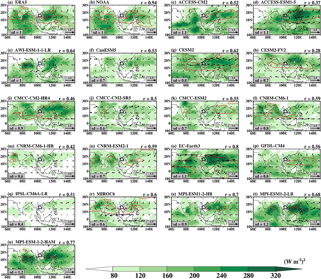
Figure 2. Variance of 30–60-day bandpass-filtered intraseasonal OLR and 850-hPa zonal wind (contour) overlaid with 30–60-day bandpass-filtered 850-hPa wind (vector) anomalies during the boreal summer (May–October) obtained from observations and CMIP6 models for the period 1997–2014. The solid red contour is the 4.0 (m s−2)2 isoline of the bandpass-filtered 850-hPa zonal wind variance. The Spearman correlation (r) of filtered OLR anomaly on (b; NOAA) and (c–u; CMIP6 models) is obtained against (a) ERA5 as the reference. The standard deviation of OLR normalized by the ERA5 standard deviation is shown at the bottom left of the plot.
Several BSISO diagnostics tools and statistics have been developed and applied to evaluate the ability of the climate models in reproducing the spatio-temporal characteristics, intensity, zonal location, and propagation behavior of the BSISO (e.g., Li and Mao, 2016; Hu et al., 2017; Qi et al., 2019). The chief among the diagnostics statistics includes the wavenumber-frequency power spectrum and the combined empirical orthogonal function (CEOF). These statistics are used in this study and have also appeared in several studies (for example, Jiang et al., 2004; Kim et al., 2009; Waliser et al., 2009; Sperber and Kim, 2012; Li, 2014; Li and Mao, 2016; Ahn et al., 2017; and references therein).
The life cycle of BSISO over the Asian summer monsoon is characterized by both the eastward and northward propagations. To focus on the propagation behavior of the BSISO, we compute the wavenumber-frequency power spectra of filtered OLR and U850 anomalies. We use the power spectra averaged over the latitudinal band of 10°S−30°N to depict the eastward/westward propagation of the BSISO, while we use the power spectra averaged over the longitudinal band of 100°E−120°E (southeast Asia) and 70°E−100°E (equatorial Indian Ocean) to depict the northward/southward propagation of the BSISO. For this computation, the power spectra are obtained for an individual half-year (180 days in length) and an averaged spectrum is computed by averaging over all the periods of the data record. Figures 3, 4 and Supplementary Figure 1 show the pattern of this statistic.
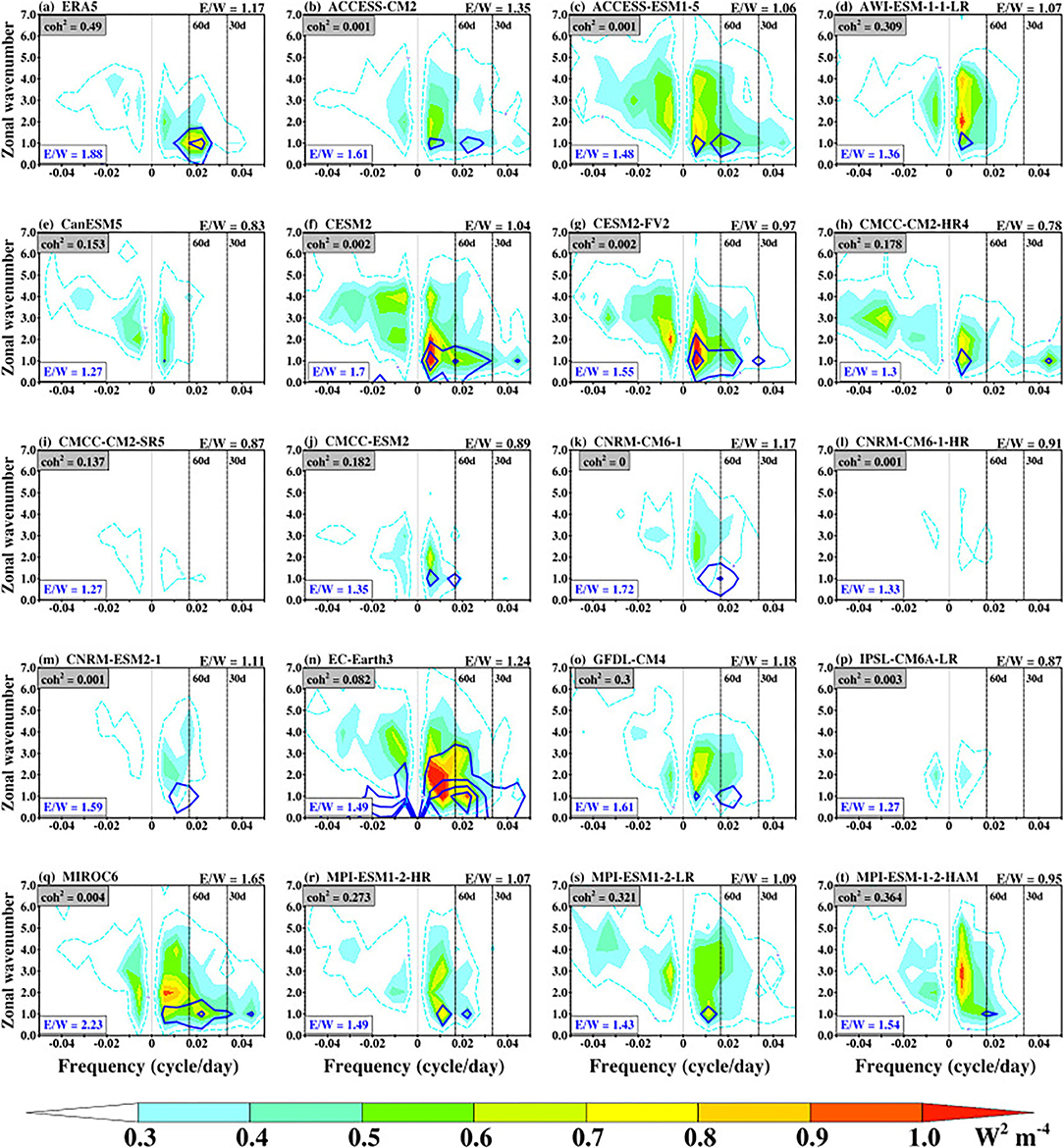
Figure 3. Zonal wavenumber-frequency power spectra of the boreal summer (May–October) intraseasonal OLR (shaded) and 850-hPa zonal wind [blue contours; (m s−1)2, with contours from 0.02 at an interval of 0.02] anomalies from observations (a; OLR and ERA5) and CMIP6 models (b–t) over 10°S−30°N domain. The cyan dotted contour represents the 0.2 (W m−2)2 isoline of OLR. Periods of 30 days and 60 days are indicated by the vertical dashed lines. Positive frequencies indicate eastward propagating waves and negative frequencies indicate westward propagating waves. The ratio of OLR eastward propagating wave to westward propagating wave (E/W) is shown at the top panel, while that of the zonal wind is shown at the bottom left (blue). The coherence-squared (Coh2) of OLR and 850-hPa zonal wind averaged over 10°S−30°N is shown at the upper left corner of the plot.
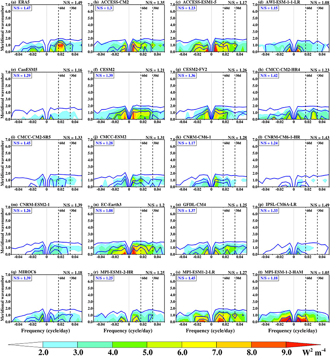
Figure 4. Meridional wavenumber-frequency power spectra of the boreal summer (May–October) intraseasonal OLR (shaded) and 850-hPa zonal wind [blue contours; (m s−1)2, with contours from 0.03 at an interval of 0.06] anomalies from observations (a; OLR and ERA5) and CMIP6 models (b–t) over 100°E−120°E domain. Periods of 30 and 60 days are indicated by the vertical dashed lines. Positive frequencies indicate northward propagating waves and negative frequencies indicate southward propagating waves. The ratio of OLR northward propagating wave to southward propagating wave (N/S) is shown at the top panel, while that of the zonal wind is shown at the upper left corner of the plot (blue).
In both NOAA and ERA5, the maximum eastward power (positive frequency) of OLR is contained at a 40–60-day period and zonal wavenumbers 1–3 (Figure 3a). The counterpart westward spectra power (negative frequency) is much smaller than that of the eastward power. This is evident by the strong Eastward/Westward power ratio (E/W ratio). Consistent with Lin et al. (2006) and Ahn et al. (2017), this skill metric is obtained as the ratio of the sum of eastward power spectra to the sum of westward power spectra over the 30–60-day band. The observed E/W ratio is >1 (1.26 and 1.17 for NOAA and ERA5, respectively), which signify the robustness of the BSISO eastward propagation. As indicated by the blue contours in Figure 3a, the observed eastward-propagating U850 spectrum is consistent with that of the OLR spectrum. However, the westward counterpart of the eastward power of U850 is weak. Here, the E/W ratio is 1.88 for ERA5. Comparing the E/W ratio for OLR with that of U850 shows that the BSISO eastward-propagating oscillation is more robust in U850 than in OLR. The CMIP6 models exhibit the spectra power of OLR over a wide range of frequencies and zonal wavenumbers. Also, the maximum power is concentrated vertically across zonal wavenumbers 1–4 in most of the models and outside the observed 40–60-day period. Although the westward-propagating power in some of the models is weaker than the eastward-propagating power, about 40% of the models overestimate the observed westward-propagating power. The simulated E/W ratio of OLR varies between 0.78 and 1.65. Four of the models, CMCC-CM2-SR5, CNRM-CM6-1-HR, CNRM-ESM2-1, and IPSL-CM6A-LR, have OLR spectra power lower than 3 W2 m−4 (Figures 3i,l,m,p), while CESM, CESM2-FV2, and EC-Earth3 have eastward-propagating signal that is considerably greater in magnitude than the observed signal, and the maximum power is located at wavenumbers 1–4 between 60 and 200-day period (Figures 3f,g,n).
Looking at the contour plot of the simulated U850 power spectrum in the models (Figures 3c–t), we see that CMIP6 models can simulate the distribution of the observed zonal wind power spectrum. However, there are differences in their magnitude. While EC-Earth3 produces excessive power spectra across wavenumbers 1–3, the models with weak OLR power spectra also exhibit a very weak U850 power spectrum (< 0.02 m2 s−2). Also, most of the CMIP6 models have a strong E/W ratio of U850, which indicates that the BSISO eastward variance of U850 dominates over the westward variance. In contrast to ERA5 and other models, EC-Earth3 produces too large U850 variances. In addition to the E/W ratio, another statistic derived from the wavenumber-frequency power spectra is the coherence-squared (Coh2). This statistic shows the consistency between the OLR and U850. To obtain this statistic, we compute the cross-spectra to quantify the coherence relationship between the two variables for the summer season on 180-day length segments, overlapping by 130 days. The result of the ERA5 symmetric component of the Coh2 spectrum between these variables, at the wavenumber-frequency space that characterizes the BSISO, is about 0.49. This shows the consistency between the low-level circulation and convection. The CMIP6 models struggle to simulate this coherence at the BSISO band. On average, the simulated Coh2 peaks at about 0.32.
The meridional propagation (northward/southward) of the BSISO over Southeast Asia represented by the meridional wavenumber-frequency power spectra of OLR and U850 is shown in Figure 4. In both the observations and the models, the meridional propagation of the power spectrum of these variables (concentrated at wavenumbers 1 and 2) is dominated by the northward propagating component as indicated by the Northward/Southward power ratio (N/S ratio). This ratio is >1 for both OLR and U850. The observed mean N/S ratio for OLR is about 1.49, while the simulated OLR N/S ratio ranges from 1.05 to 1.49. This metric is of the same order for U850, where the observed mean N/S ratio is about 1.47 and the simulated N/S ratio ranges from 1.08 to 1.45. Unlike the zonal propagation (Figure 3), there is a strong correspondence between OLR and U850 at the BSISO characteristic band. Comparing Figures 3, 4, it is reasonable to state that the meridional propagation of the BSISO is more robust than the zonal propagation over the tropical domain between 5°S−20°N and 100°E−120°E. The structure of the meridional propagation of the BSISO over the equatorial Indian Ocean (Supplementary Figure 1) is similar to that of Figure 4. The slight differences in magnitude and the value of the N/S ratio between Figure 4 and Supplementary Figure 1 further confirm the separate influence of the BSISO over the two regions.
The first part of this section presents the statistics and the spatial structures (normalized eigenvectors) of the first two leading modes of the combined empirical orthogonal functions (CEOFs) derived from the 30–60-day bandpass-filtered anomalies of OLR and U850 variables. The second part focuses on the real-time multivariate BSISO index.
The individual and total variances of OLR and U850 explained by each CEOFs are presented in Table 3. In ERA5, the first two leading CEOF modes explain about 20% each of the total variance of the combined variables, which indicates that they form a pair describing a propagating signal. Looking at the variance of individual variables explained by CEOF1 and CEOF2, OLR explained variance is the least and U850 explained variance is the most. The CMIP6 models show a wide range of the individual and total variances explained by the CEOF. For OLR, on average, the magnitude of the explained variance is smaller compared to the observed, as well as in comparison to U850. This indicates that models find it difficult to produce coherent OLR variability associated with the BSISO. This disparity may be related to the different convection parameterization schemes in the models.

Table 3. Variance explained by the combined empirical orthogonal functions.
Figure 5 shows the observed and simulated eigenvectors of the CEOFs from which the above statistics are obtained. Pre-analysis of the CEOFs shows that simulated CEOF2 leads CEOF1 in some of the models. Hence, for consistency with the structure of ERA5, we switch the sign and order of some simulated CEOFs. As indicated by ERA5, CEOF1 depicts positive OLR anomaly concentrated over the longitudes of the Indian Ocean, with a peak at about 70°E, and negative OLR anomaly over the longitudes of Southeast Asia (Figure 5A). This feature is associated with weak easterlies and strong westerlies over most parts of the Indian Ocean and the Pacific (Figure 5B). For the CEOF2, the OLR is positive over both the Indian Ocean and the Pacific region. However, the associated low-level wind is a strong easterly and westerly wind component over the two oceanic regions, respectively (Figures 5C,D). The similarity in the structures of the simulated eigenvectors of the CEOFs with those of ERA5 indicates the ability of CMIP6 models in reproducing the spatial patterns of BSISO. However, some of the models still struggle with the magnitude of this statistic.
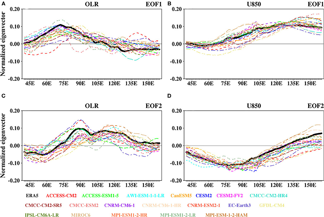
Figure 5. The normalized eigenvectors of the first two leading modes of the combined empirical orthogonal functions (CEOFs) of 30–60-day 10°S−30°N domain averaged OLR and U850 for ERA5 (solid black line) and CMIP6 models (dashed color lines). (A,B) are for the first mode and (C,D) are for the second mode. The sign and order of some of the simulated CEOFs are switched to resemble that of ERA5 (see section The CEOF and PC analyses for details).
We present the observed and simulated lead-lag correlations between the principal component time series (otherwise known as the real-time multivariate BSISO index) of the first two leading CEOF modes in Figure 6. Here the PCs are calculated by projecting the filtered CEOF eigenvector onto the bandpass-filtered daily anomaly fields. At a lag of about 10 days, the maximum correlation between the PCs is about 0.6, where PC1 leads PC2, and vice versa. Consistent with the literature, the phase quadrature between the PCs indicates the coherent northward-propagation of the BSISO at the intraseasonal timescale (Lee et al., 2013). The simulated maximum correlation ranges from about 0.3–0.7. The models show the ability to capture the spatial pattern of the observed lag correlation, but with biases in the lead-lag days.
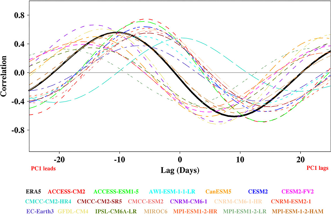
Figure 6. The lag correlation between the first two leading PCs during the boreal summer (May–October) obtained from ERA5 and CMIP6 models for the period 1997–2014.
Are the filtered CEOF modes presented in Figure 5 distinguishable from a red noise? It is known that red noise can sometimes masquerade as a distinct structure of the intraseasonal variability of the leading CEOFs. To examine this, we compute the power spectra and cross spectra (coherence squared) of the PCs of the first two leading modes. Figure 7 shows the patterns of the power spectra and equivalent variance red noise spectra, with the ordinate axis as a ratio of variance to frequency, superimposed with the coherence squared. Both the observed and the simulated power spectrum are concentrated at a 30–60-day period with a peak at about 40-day. The fraction of the red noise within the BSISO intraseasonal time scale is considerably lower, suggesting that CEOF modes are separated from red noise. The contrast between these features increases the confidence that the CEOF modes are physically based and represent the associated BSISO intraseasonal frequencies. Another important diagnostic tool to support the above result is the coherence-squared. The similarities between the structures of ERA5 Coh2 and the PC1 power spectra suggest that fluctuations of the PCs in the intraseasonal band is very coherent. Some of the CMIP6 models overestimate the observed variability of the Coh2 while others underestimate it. Overall, the models show the ability to capture the structure of this statistic. The CEOF and PC analysis indicates that models can simulate BSISO with a propagating rainfall pattern associated with moisture convergence and with a distinct time scale of 30–60 days.
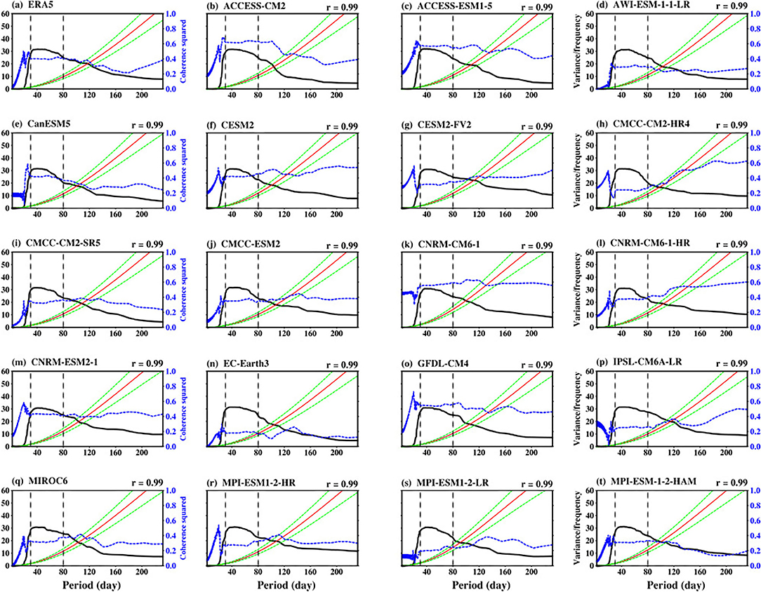
Figure 7. ERA5 (a) and CMIP6 models (b–t) power spectrum (solid black line) and coherence squared (dashed blue line) of the filtered PC1 (EOF1) obtained by projecting the 30–60-day filtered CEOFs onto 30–60-day daily anomaly data. The red noise spectrum (solid red line) and the 5 and 95% confidence limits (dashed green lines) are also indicated.
A further diagnostic to evaluate how well the models can represent the intraseasonal variability of the BSISO signal is through the Hovmöller diagrams. Here we examine the phase-longitude Hovmöller diagram of the composite of 30–60-day bandpass-filtered OLR and U850 anomalies averaged between 10°S and 30°N during May–October (Figure 8). The zonal signature of the BSISO is discernible in ERA5 (Figure 8a). The convection propagates eastward with maximum centres located over the Indian Ocean and the Southeast Asia region. The enhanced convection over the longitude of the Indian Ocean occurs during phases 1, 2, and 8, while it occurs at phase 3 over Southeast Asia. On the other hand, the suppressed convection occurs during phases 3–5, and 6–8 over the two regions, respectively. These tripole structures of the convection signify the onset/break periods of the monsoon over the regions. The structure of the low-level zonal wind is almost in quadrature with the OLR, showing that the westerly (easterly) winds are associated with negative (positive) BSISO convection. All the CMIP6 models in this study capture the zonal structure and orientation of the observed convection and low-level wind. The magnitude of the simulated convection is weak in some of the models. Also, the phases of the maximum convection are diverse.
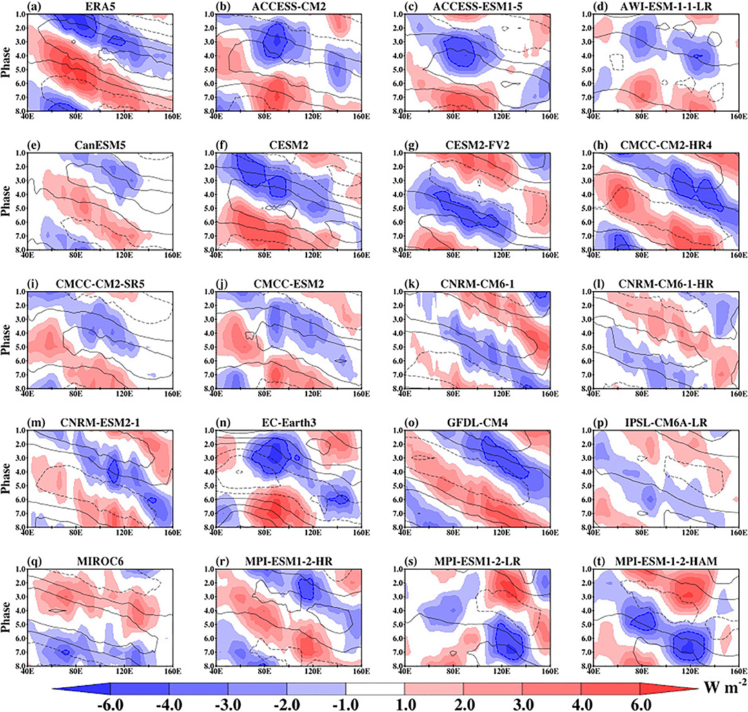
Figure 8. ERA5 (a) and CMIP6 models (b–t) phase-longitude Hovmöller plot of composite May-October 30–60-day OLR (shaded) and U850 (contour) anomalies averaged between 10°S and 30°N.
Consistent with the zonal propagation, the meridional propagation of BSISO averaged over the Indian Ocean is characterized by strong negative (positive) convection at phases 1, 2, and 8 (3–6), respectively (Figure 9). The signal starts from the equatorial region and extends as far as latitude 25°N. The CMIP6 models also show the ability to reproduce the northward propagation of the BSISO over the Indian Ocean domain. The convection signal is weak in CNRM-CM6-1-HR, IPSL-CM6A-LR, and MPI-ESM1-2-LR. When we repeat the analysis over the Southeast Asia domain (Supplementary Figure 2), we find a similar northward propagation consistent with that of the Indian Ocean domain, although the propagation extends beyond latitude 25°N.
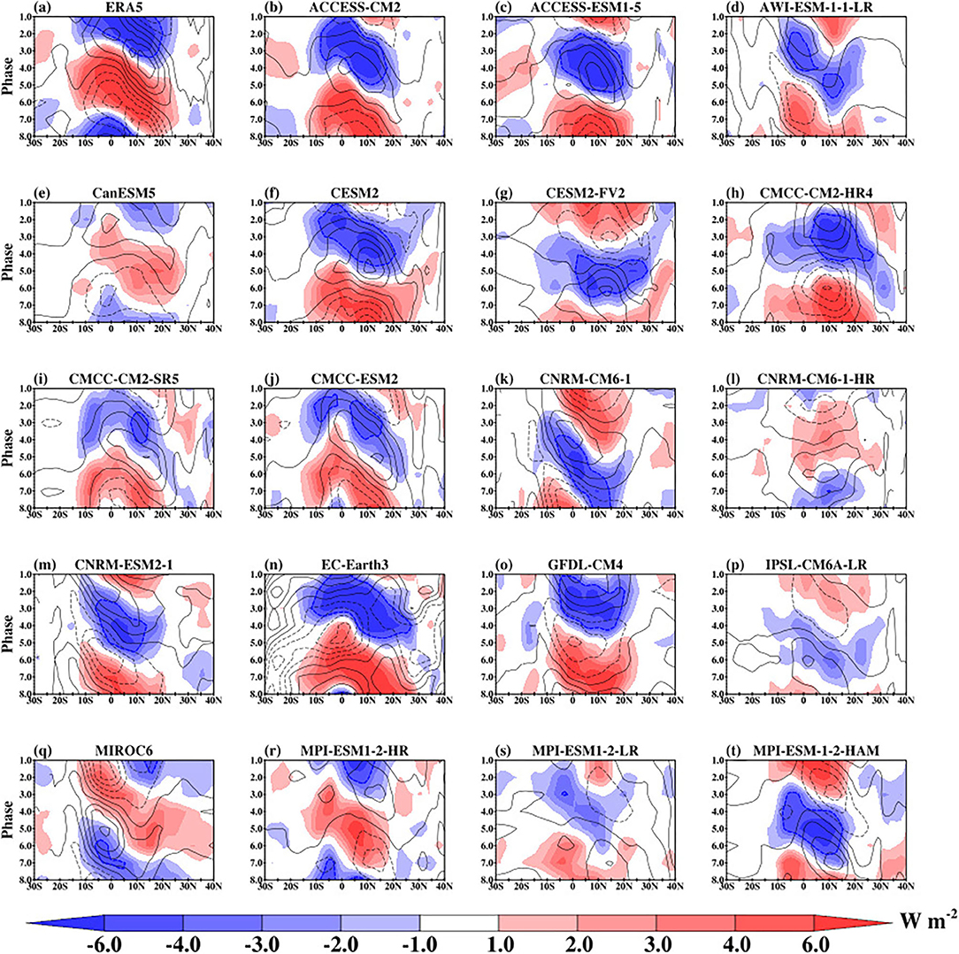
Figure 9. ERA5 (a) and CMIP6 models (b–t) phase-latitude Hovmöller plot of composite May-October 30–60-day OLR (shaded) and U850 (contour) anomalies averaged between 80°E and 100°E.
The relationship between rainfall and column MSE, DSE, and LSE over the Southeast Asia region and Indian Ocean domain is examined by lag-correlation. The simulated MSE is computed for 11 CMIP6 models with complete data at surface and the required atmospheric pressure levels.
Figure 10 shows the northward propagation of observed and simulated BSISO convection signal represented by lag correlation of 80°E−100°E averaged column integrated MSE and band-pass filtered anomalous rainfall against anomalous filtered rainfall index. The index is obtained from the band-pass filtered rainfall anomalies averaged over the equatorial Indian Ocean (5°S and 5°N, 80°E and 100°E). The rainfall anomaly in ERA5 (Figure 10a; contour) shows a clear northward propagation that transverse from about 10°S reaching the northern limit at about 20°N consistent with Figure 9a. The intraseasonal rainfall signal is stronger along the equatorial region with maxima at three lag days (−20, 0, and 20). This characteristic feature signifies the active/break of the monsoon period (Straub and Kiladis, 2003; Fang et al., 2017). A similar pattern is displayed by the column integrated MSE. The CMIP6 models can display a northward propagation of the intraseasonal rainfall and column integrated MSE consistent with ERA5. However, there are two distinct biases. First, the magnitude of the lag correlation between rainfall and column integrated MSE anomalies is slightly weaker than observed. Secondly, the northward propagating signal is limited in some of the CMIP6 models (for example, CanESM5, CNRM-CM6-1-HR, IPSL-CM6A-LR, and MPI-ESM1-2-HR) with peak values between 5°S and 15°N. These 4 models also have slightly weak OLR and not well-organized convection in comparison with other CMIP6 models as indicated in Figure 9. The northward propagation of the observed and simulated relationship between rainfall and column DSE and LSE are presented in Supplementary Figures 3, 4. The observed and simulated correlation between DSE and rainfall (Supplementary Figure 3) is very small suggesting a weak contribution from temperature and height variations to column MSE. However, the column LSE dominates the column MSE variation as indicated by Supplementary Figure 4. The correlation shows a similar pattern consistent with Figure 10, suggesting a strong relationship between rainfall and column integrated moisture, as noted in other studies (Schiro et al., 2016; Wang et al., 2017). The lag correlation between the column integrated MSE and band-pass filtered anomalous rainfall against anomalous filtered rainfall index over the Southeast Asia region is presented in Figure 11. The observed patterns (both MSE and rainfall) over this region are similar to those over the Indian Ocean (Figure 10), although the correlation between MSE and rainfall is weaker. Apart from producing a weak correlation, 3 of the models (for example, CanESM5, CESM2-FV2, and MPI-ESM1-2-HR) struggle to capture the coherent northward propagation of the relationship between MSE and rainfall. It appears that the models perform poorly in this respect over this region compared with over the Indian Ocean.
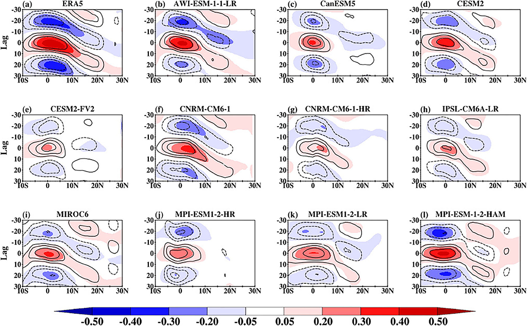
Figure 10. Northward propagation of observed and simulation BSISO convection signal indicated by column integrated MSE (shaded) and 30–60-day rainfall anomalies (contours; starting from ± 0.2 to ± 0.6 at an interval of 0.2) averaged over 80°E−100°E by lag-correlation against 30–60-day rainfall anomalies averaged over the equatorial Indian Ocean (5°S and 5°N, 80°E and 100°E).
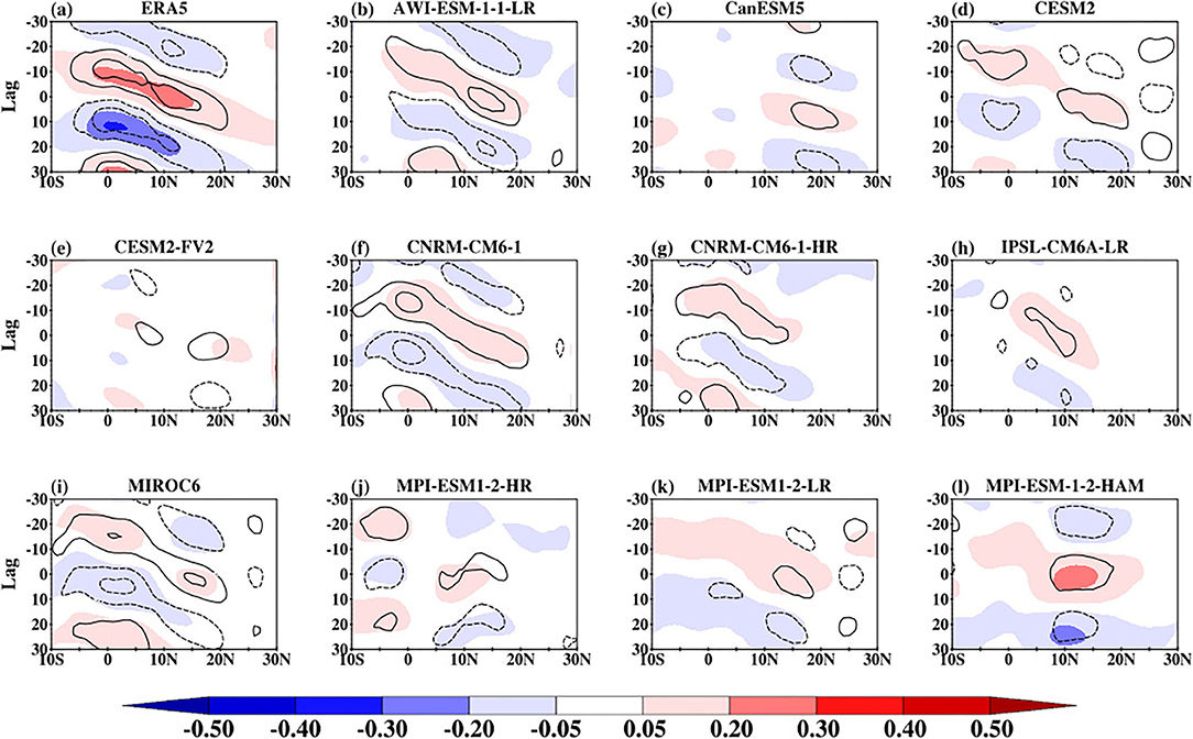
Figure 11. Northward propagation of observed (a) and simulation (b–l) BSISO convection signal indicated by column integrated MSE (shaded) and 30–60-day rainfall anomalies (contours; starting from ± 0.2 to ± 0.6 at an interval of 0.2) averaged over 100°E–120°E by lag-correlation against 30–60-day rainfall anomalies averaged over the southeast Asia (5°N and 20°N, 100°E and 120°E).).
As in Figure 10, the eastward propagation of observed and simulated equatorial (10°S−10°N averaged) column integrated MSE and rainfall anomalies lag-correlated against anomalous filtered rainfall index is presented in Figure 12. In ERA5, both the intraseasonal rainfall and column integrated MSE show coherent eastward propagation signal with a maximum correlation over the Indian Ocean domain and a weak correlation over the Pacific Ocean between 120°E and 160°E. The simulated eastward features are consistent with ERA5, but all the models have a weaker MSE correlation in comparison with that of ERA5. The supporting Supplementary Figure 5 also confirms that the contribution from the column DSE to the column MSE is very small, while Supplementary Figure 6 shows the dominant contribution of column LSE to the column MSE relationship with rainfall.
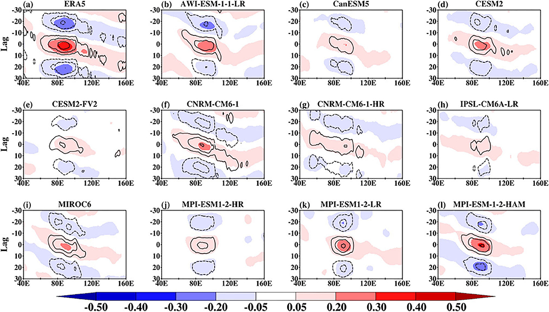
Figure 12. Eastward propagation of observed (a) and simulation (b–l) BSISO convection signal indicated by column integrated MSE (shaded) and 30-60-day rainfall anomalies (contours; starting from ± 0.2 to ± (a) 0.6 at an interval of 0.2) averaged over 10°S−10°N by lag-correlation against 30–60-day rainfall anomalies averaged over the equatorial Indian Ocean (5°S and 5°N, 80°E and 100°E).
The results show that the CMIP6 models can capture the intraseasonal propagating features of BSISO with high prominence in the northward propagation, a significant measure of the skill of the model to simulate BSISO. Also, the result shows there is a strong relationship between MSE and rainfall, with the largest contribution from LSE. This suggests that MSE can be used as a proxy for propagating BSISO convective signal consistent with MJO studies (Jiang, 2017).
The above analysis revealed the strengths and weaknesses of CMIP6 climate models at simulating the boreal summer intraseasonal oscillations over the SE Asia region. It shows that some CMIP6 models underestimated the basic characteristic features of BSISO. Several physical processes including the vertical shear of zonal wind, variation of background mean state, air-sea interaction, and boundary layer dynamics have been suggested to play a key role in influencing the simulation and propagation of intraseasonal oscillations (Fu and Wang, 2004; Benedict et al., 2014; Jiang et al., 2015; Fan et al., 2021). To explore the deficiency in simulated BSISO, we examine the distribution of some mean fields (rainfall, specific humidity, and MSE). These fields are considered because they are directly related to convection and also because the column LSE dominates the distribution of the column MSE.
All the models show mean rainfall that is spatially similar with each other as well as with the GPCP as indicated by the pattern correlation that ranges from 0.45 to 0.74. Despite the similarities in patterns, there are still local differences in rainfall intensity with the rmse that ranges from 1.91 to 3.09 (Supplementary Figure 7). Some of the models show clear weakness in simulating the mean rainfall over the mountainous region of India and the Oceanic regions. For instance, ACCESS-CM2 (Figure 13b), ACCESS-ESM1-5 (Figure 13c), and CanESM5 underestimate mean rainfall by more than 2 mm month−1. The models also overestimate mean rainfall by more than 2 mm month−1 over the Pacific region. Considering the mean bias over the domains used to examine the BSISO propagation, we note that the CMCC, CNRM-CERFACS, and IPSL models on average underestimate the mean rainfall over SE Asia, while other models overestimate the mean rainfall with the highest mean rainfall bias (> 1.40 mm month−1) in 4 models (ACCESS-CM2, ACCESS-ESM1-5, AWI-ESM1-1-LR, and CanESM5). These indicate that the models' convective parameterization schemes, respectively, underestimate/overestimate the convective quantities including the moisture convergence flux and the convective available potential energy. Hence, the models may exhibit differences in their moisture distributions. The spatial distribution of mean specific humidity at 850 hPa level is shown in Supplementary Figure 8. We note that the CMIP6 models can simulate the spatial pattern of the mean specific humidity (pattern correlation ranges from 0.69 to 0.93), relative to ERA5, but with some notable biases (rmse ranges from 0.70 to 1.87) (Supplementary Figure 8). Consistent with the mean rainfall bias, Figure 14 shows that some CMIP6 models are wet bias while others are dry bias. A dipole moisture bias is also evident where the land regions are deficient in moisture while the oceanic regions are characterized by abundant moisture content, relative to ERA5. The poor performance of the models in representing the mean state is reflected in their inability to quantitatively reproduce the intraseasonal oscillations (e.g., Figures 1, 2). These suggest that the models' sufficient moisture for rainfall. Also, the dry biases over land suggest that the models do not transport enough moisture northward, which may be related to the land surface processes (e.g., evaporation) and the land-sea temperature contrast. The spatial distributions of the simulated biases of the vertically integrated MSE (Figure 15) are consistent with that of the moisture biases (Figure 14), confirming the close relationship between the MSE and the convection systems producing rainfall. From the foregoing, we can infer that models' inability to qualitatively capture the background mean states may likely explain the inability to satisfactorily capture the intraseasonal oscillations during summer.
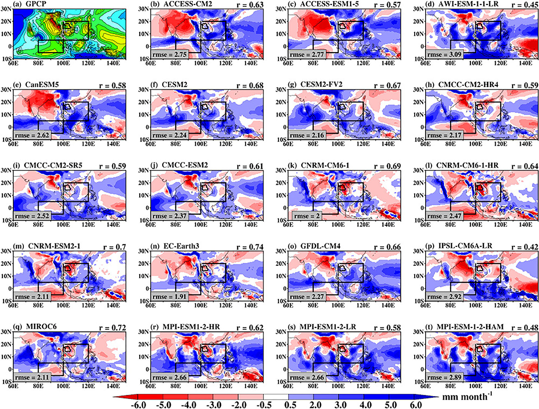
Figure 13. The bias in the simulated monthly mean rainfall (b–t) with reference to GPCP (a) during May–October 1997–2014. The mean pattern of GPCP rainfall is indicated for reference. The pattern correlation (r) and the root mean squared error (rmse) values between the simulated patterns and that of GPCP in Supplementary Figure 1 are indicated for reference.
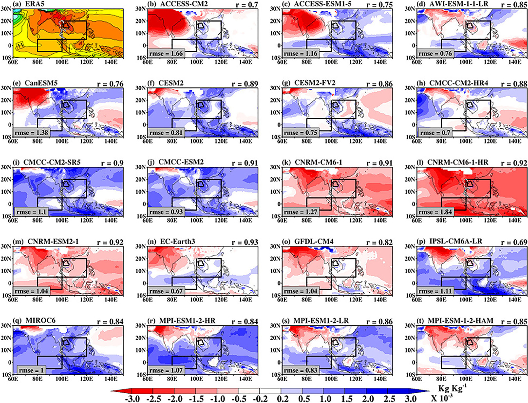
Figure 14. The bias in the simulated monthly mean specific humidity at 850 hPa (b–t) with reference to ERA5 (a) during May–October 1997–2014. The mean pattern of ERA5 specific humidity at 850 hPa is indicated for reference. The pattern correlation (r) and the root mean squared error (rmse) values between the simulated patterns and that of ERA5 in Supplementary Figure 2 are indicated for reference.
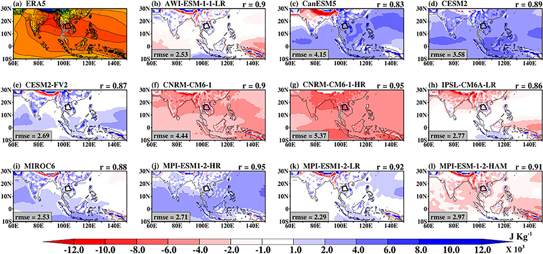
Figure 15. The bias in the simulated monthly mean vertically integrated moist static energy (b–l) with reference to ERA5 (a) during May–October 1997–2014. The mean pattern of ERA5 vertically integrated moist static energy is indicated for reference. The pattern correlation (r) and the root mean squared error (rmse) values between the simulated patterns and that of ERA5 in Supplementary Figure 3 are indicated for reference.
How well the features associated with BSISO are represented in 19 CMIP6 models is the focus of this study. This has been achieved by employing the MJOWG diagnostic tools. The simulated results are evaluated against GPCP, NOAA, and ERA5 data sets.
Analysis of GPCP and ERA5 rainfall shows that there are observational uncertainties that are very important for model evaluation. The maximum GPCP rainfall variance over the East China Sea and the western Pacific Ocean are shown to be consistent with other studies (Zhang et al., 2006). The similarities in intraseasonal rainfall variance between the GPCP and ERA5 indicate the usefulness of this reanalysis variable for climate model evaluation. The two observed datasets agree that BSISO can account for more than 10% of the intraseasonal rainfall variability over the region. The intraseasonal variance of bandpass-filtered rainfall anomalies is well-captured by most of the CMIP6 models, while it is underestimated in others. Some models including the CNRM group of models, ACCESS-ESM1-5, and MIROC6 overestimate the rainfall variance over the coastal regions. The overestimation suggests that the localized convective systems in these models are too strong over the coastal regions, while weak over the land region. This behavior is consistent with the models' rainfall failure over India (Mitra, 2021). Also, the difference among the models may be related to the differences in their representation of hydrological processes (Klutse et al., 2021). Considering the OLR variance, a close relationship is seen between convection and rainfall, where low (high) OLR variance coexist with low (high) rainfall variance over Thailand and the maritime continent (Oceanic regions). This is supported by the intraseasonal low-level zonal wind associated with the weak westerlies over land and strong westerlies over the Ocean areas. The CMIP6 models simulate the intraseasonal variance of bandpass-filtered OLR, but CNRM-CM6-1-HR and IPSL-CM6A-LR underestimate the magnitude of the OLR over the Indian Ocean.
As indicated by the variance analysis, some of the CMIP6 models can simulate the intraseasonal variability of the BSISO with strong intensity over the tropical rain belt. However, are these models also able to quantify the properties of the BSISO including the wavenumber-frequency power spectra and coherence squared? The equatorially averaged wavenumber-frequency power spectra of observed convection and low-level zonal wind circulation coincide at zonal wavenumber 1 within the 40–60-day period. This is supported by a considerably weaker mean westward power spectra. The strong ratio of eastward to westward power signifies the robustness of the observed BSISO eastward propagation feature. The CMIP6 models can simulate the BSISO features, but with diverse power spectra over a wide range of frequencies and zonal wavenumbers. Consistent with observation, the simulated eastward power is higher than the counterpart westward power. Some models overestimate this statistic while others underestimate it. CMCC-CM2-SR5, CNRM-CM6-1-HR, CNRM-ESM2-1, and IPSL-CM6A-LR exhibit low OLR spectra power (<3 W2 m−4), consistent with their poor performance of spatial variance. The structure of the meridional propagating BSISO at wavenumbers 1 and 2 over both the Southeast Asia and the Indian Ocean regions is well-simulated by the CMIP6 models, but with bias in intensity and location. This is indicated by the simulated N/S ratio that encompasses the observed N/S ratio. Nonetheless, some models still have weaker northward propagating BSISO convection signals.
Considering the eigenvectors of the first two leading modes of the CEOFs, it is shown that the models also capture the longitudinal structure of these two indices, with PC1 leading PC2 by about 10-days. The observed eigenvector is contained within the spread of the models, with some models leading (lagging) observation by about 5-days. The models also show the ability to simulate the power spectrum and coherence squared of the PC1. Also, the distinction between the CEOF modes and the red noise is equally well-captured. The similarities between the observed and simulated CEOFs, as well as the PCs, suggest that CMIP6 models can capture the coherent intraseasonal propagating features of the BSISO, in agreement with other modeling studies of the BSISO. This attribute sheds light on the future utility of some of the models to provide an understanding of the impact of BSISO variability on climate variability (e.g., rainfall, temperature, etc.) at the regional scale.
As indicated by the Hovmöller diagram of the composite of 30–60-day bandpass-filtered OLR and U850 anomalies, the CMIP6 models can simulate the zonal propagation of the BSISO with maximum centres located over the Indian Ocean and the Southeast Asia region. Some of the models can simulate the robust eastward propagation of convection and associated winds, although the convection is weak. We note also that the CMIP6 models perform well at simulating the northward propagation of BSISO signal over the aforementioned regions.
On the relationship between MSE and intraseasonal rainfall anomalies, we show that MSE can be used as a proxy to characterize propagating BSISO convective signal. However, there is a wide inter-model variability in comparison with observation, which is discernible over the Southeast Asia region. Decomposing the MSE into separate components, we find that most of the variations in MSE with rainfall are largely attributed to the contribution from the LSE. The variations from the DSE is negligible indicating the weak temperature gradient in the tropics. Hence, the BSISO rainfall is mainly influenced by large-scale processes controlling the atmospheric column humidity over the region.
In summary, by applying the simulation diagnostics developed by the CLIVAR MJOWG to 19 CMIP6 models, with promising future simulation data, we examine the strengths and weaknesses of these models at simulating the intraseasonal variability of the basic features of the BSISO. In general, the BSISO signal is stronger in the low-level wind circulation than in convection in both the observation and the models. The strong diversity in the intensity of both the simulated eastward and northward propagation of BSISO convection indicates that the CMIP6 models still struggle to simulate the physical processes, including moisture asymmetry and vertical wind shear, responsible for the BSISO propagating features (Liu and Wang, 2017; Qi et al., 2019). Despite some limitations noted in the CMIP6 models, some of the models still offer promising utility for climate research. Hence, our forthcoming research will investigate the impact of climate change on the BSISO and its potential impact on rainfall over Southeast Asia.
The original contributions presented in the study are included in the article/Supplementary Material, further inquiries can be directed to the corresponding author.
AA, MC, MB, DK, and YD contributed to the conception and design of the paper. AA performed the analysis and writing of the paper. All authors contributed to paper revision and approved the work for publication.
This work was part of the ENRICH (ENhancing Resilient to future Hydrometeorological extremes in the Mun river basin in Northeast of Thailand) project supported by the U.K. Natural Environment Research Council/Newton fund under NE/S002901/1 and by the Thailand Science Research and Innovation/National Research Council of Thailand under RDG6130025.
The authors declare that the research was conducted in the absence of any commercial or financial relationships that could be construed as a potential conflict of interest.
All claims expressed in this article are solely those of the authors and do not necessarily represent those of their affiliated organizations, or those of the publisher, the editors and the reviewers. Any product that may be evaluated in this article, or claim that may be made by its manufacturer, is not guaranteed or endorsed by the publisher.
The authors appreciate the U.S. CLIVAR MJO Working Group and the National Center for Atmospheric Research Command Language team for the availability of the MJO simulation diagnostics scripts. We thank all the reviewers for their helpful comments.
The Supplementary Material for this article can be found online at: https://www.frontiersin.org/articles/10.3389/fclim.2021.716129/full#supplementary-material
Supplementary Figure 1. Meridional wavenumber-frequency power spectra of the boreal summer (May–October) intraseasonal OLR (shaded) and 850-hPa zonal wind [blue contours; (m s−1)2, with contours from 0.03 at an interval of 0.06] anomalies from observations and models over 80°E−100°E domain. Periods of 30 days and 60 days are indicated by the vertical dashed lines. Positive frequencies indicate northward propagating waves and negative frequencies indicate southward propagating waves. The ratio of northward propagating wave to southward propagating wave (N/S) is shown at the top panel.
Supplementary Figure 2. Phase-latitude Hovmöller plot of composite May–October 30–60-day OLR (shaded) and U850 (contour) anomalies averaged between 100°E and 120°E.
Supplementary Figure 3. Northward propagation of observed and simulation BSISO convection signal indicated by column integrated DSE (shaded) and 30–60-day rainfall anomalies (contours; starting from ± 0.2 to ± 0.6 at an interval of 0.2) averaged over 80°E–100°E by lag-correlation against 30–60-day rainfall anomalies averaged over the equatorial Indian Ocean (5°S and 5°N, 80°E and 100°E).
Supplementary Figure 4. Northward propagation of observed and simulation BSISO convection signal indicated by column integrated LSE (shaded) and 30–60-day rainfall anomalies (contours; starting from ± 0.2 to ± 0.6 at an interval of 0.2) averaged over 80°E–100°E by lag-correlation against 30–60-day rainfall anomalies averaged over the equatorial Indian Ocean (5°S and 5°N, 80°E and 100°E).
Supplementary Figure 5. Eastward propagation of observed and simulation BSISO convection signal indicated by column integrated LSE (shaded) and 30–60-day rainfall anomalies (contours; starting from ± 0.2 to ± 0.6 at an interval of 0.2) averaged over 10°S−10°N by lag-correlation against 30–60-day rainfall anomalies averaged over the equatorial Indian Ocean (5°S and 5°N, 80°E and 100°E).
Supplementary Figure 6. Eastward propagation of observed and simulation BSISO convection signal indicated by column integrated DSE (shaded) and 30–60-day rainfall anomalies (contours; starting from ± 0.2 to ± 0.6 at an interval of 0.2) averaged over 10°S−10°N by lag-correlation against 30–60-day rainfall anomalies averaged over the equatorial Indian Ocean (5°S and 5°N, 80°E and 100°E).
Supplementary Figure 7. The observed and simulated monthly mean rainfall during May–October 1997–2014. The pattern correlation (r) and the root mean squared error (rmse) values between the simulated patterns and that of GPCP are indicated.
Supplementary Figure 8. The observed and simulated monthly mean specific humidity at 850 hPa during May–October 1997–2014. The pattern correlation (r) and the root mean squared error (rmse) values between the simulated patterns and that of ERA5 are indicated.
1. ^http://www.ncl.ucar.edu/Applications/mjoclivar.shtml
2. ^https://climatedataguide.ucar.edu/climate-data-tools-and-analysis/empirical-orthogonal-function-eof-analysis-and-rotated-eof-analysis
Abhik, S., Mukhopadhyay, P., Krishna, R. P. M., Salunke, K. D., Dhakate, A. R., and Rao, S. A. (2016). Diagnosis of boreal summer intraseasonal oscillation in high resolution NCEP climate forecast system. Clim. Dyn. 46, 3287–3303. doi: 10.1007/s00382-015-2769-9
Ahn, M.-S., Kim, D., Kang, D., Lee, J., Sperber, K. R., Gleckler, P. J., et al. (2020). MJO propagation across the Maritime Continent: Are CMIP6 models better than CMIP5 models? Geophys. Res. Lett. 47:e2020GL087250. doi: 10.1029/2020GL087250
Ahn, M.-S., Kim, D., Sperber, K. R., Kang, S., Maloney, E., Waliser, D., et al. (2017). MJO simulation in CMIP5 climate models: MJO skill metrics and process-oriented diagnosis. Clim. Dyn. 49, 4023–4045. doi: 10.1007/s00382-017-3558-4
Alaka, G. J., and Maloney, E. D. (2012). The Influence of the MJO on Upstream Precursors to African Easterly Waves. J. Climate 25, 3219–3236. doi: 10.1175/JCLI-D-11-00232.1
Annamalai, H., and Sperber, K. R. (2005). Regional heat sources and the active and break phases of boreal summer intraseasonal (30-50 day) variability. J. Atmos. Sci. 62, 2726–2748. doi: 10.1175/JAS3504.1
Benedict, J. J., Maloney, E. D., Sobel, A. H., and Frierson, D. M. W. (2014). Gross moist stability and MJO simulation skill in three full-physics GCMs. J. Atmos. Sci. 71, 3327–3349. doi: 10.1175/JAS-D-13-0240.1
Duffy, P. B., Govindasamy, B., Iorio, J. P., Milovich, J., Sperber, K. R., Taylor, K. E., et al. (2003). High-resolution simulations of global climate, part 1: present climate. Clim. Dyn. 21, 371–390. doi: 10.1007/s00382-003-0339-z
Ellingson, R. G., Yanuk, D. J., Lee, H.-T., and Gruber, A. (1989). A technique for estimating outgoing longwave radiation from HIRS radiance observations. J. Atmos. Ocean. Tech. 6, 706–711. doi: 10.1175/1520-0426(1989)006<0706:ATFEOL>2.0.CO;2
Eyring, V., Bony, S., Meehl, G. A., Senior, C. A., Stevens, B., Stouffer, R. J., et al. (2016b). Overview of the Coupled Model Intercomparison Project Phase 6 (CMIP6) experimental design and organization. Geosci. Model Dev. 9, 1937–1958. doi: 10.5194/gmd-9-1937-2016
Eyring, V., Righi, M., Lauer, A., Evaldsson, M., Wenzel, S., and Jones, C. (2016a). ESMValTool (v1.0) - a community diagnostic and performance metrics tool for routine evaluation of Earth system models in CMIP. Geosci. Model Dev. 9, 1747–1802. doi: 10.5194/gmd-9-1747-2016
Fan, Y., Kan, F., and Xu, Z. (2021). Intraseasonal oscillation intensity over the western North Pacific: Projected changes under global warming. Atmos. And Oceanic Sci. Lett. 14:100046. doi: 10.1016/j.aosl.2021.100046
Fang, Y., Wu, P., Mizielinski, M. S., Roberts, MJ, Wu, T., Li, B., Vidale, P. L., et al. (2017). High-resolution simulation of the boreal summer intraseasonal oscillation in Met Office Unified model. Q. J. R. Meteorol. Soc. 143, 362–373. doi: 10.1002/qj.2927
Fu, X. H., and Wang, B. (2004). Differences of boreal summer intraseasonal oscillations simulated in an atmosphere-ocean coupled model and an atmosphere-only model. J. Climate. 17, 1263–1271. doi: 10.1175/1520-0442(2004)017<1263:DOBSIO>2.0.CO
Hersbach, H., Bell, B., Berrisford, P., Hirahara, S., Horányi, A., Muñoz-Sabater, J., et al. (2020). The ERA5 global reanalysis. Q. J. R. Meteorol. Soc. 146, 1999–2049. doi: 10.1002/qj.3803
Higgins, R. W., and Shi, W. (2001). Intercomparison of the principal modes of interannual and intraseasonal variability of the North American monsoon system. J. Climate 14, 403–417. doi: 10.1175/1520-0442(2001)014<0403:IOTPMO>2.0.CO
Hsu, P. C., and Li, T. (2011). Interactions between boreal summer intraseasonal oscillations and synoptic-scale disturbances over the western North Pacific. Part II: Apparent heat and moisture sources and eddy momentum transport. J. Clim. 24, 942–961. doi: 10.1175/2010JCLI3834.1
Hu, W., Duan, A., and He, B. (2017). Evaluation of intra-seasonal oscillation simulations in IPCC AR5 coupled GCMs associated with the Asian summer monsoon. Int. J. Climatol. 37, 476–496. doi: 10.1002/joc.5016
Huffman, G. J., Adler, R. F., Morrissey, M. M., Bolvin, D. T., Curtis, S., Joyce, R., et al. (2001). Global precipitation at one degree daily resolution from multisatellite observations. J. Hydrometeor. 2, 36–50. doi: 10.1175/1525-7541(2001)002<0036:GPAODD>2.0.CO
Hung, M.-P., Lin, J.-L., Wang, W., Kim, D., Shinoda, T., and Weaver, S. J. (2013). MJO and convectively coupled equatorial waves simulated by CMIP5 climate models. J. Climate 26, 6185–6214. doi: 10.1175/JCLI-D-12-00541.1
Inness, P. M., and Slingo, J. M. (2003). Simulation of the madden-julian oscillation in a coupled general circulation model. Part I: comparison with observations and an atmosphere-only, GCM. J. Climate 16, 345–364. doi: 10.1175/1520-0442(2003)016<0345:SOTMJO>2.0.CO
Inness, P. M., Slingo, J. M., Guilyardi, E., and Cole, J. (2003). Simulation of the Madden-Julian Oscillation in a Coupled General Circulation Model. Part II: The role of the basic state. J. Climate 16, 365–382. doi: 10.1175/1520-0442(2003)016<0365:SOTMJO>2.0.CO
Jena, P., Azad, S., and Rajeevan, M. N. (2016). CMIP5 projected changes in the annual cycle of Indian monsoon rainfall. Climate 4:14. doi: 10.3390/cli4010014
Jiang, X. (2017). Key processes for the eastward propagation of the Madden-Julian Oscillation based on multimodel simulations. J. Geophys. Res. Atmos. 122, 755–770. doi: 10.1002/2016JD025955
Jiang, X., Waliser, D. E., Xavier, P. K., Petch, J., Klingaman, N. P., Woolnough, S. J., et al. (2015). Vertical structure and physical processes of the Madden-Julian oscillation: Exploring key model physics in climate simulations. J. Geophys. Res. Atmos. 120, 4718–4748. doi: 10.1002/2014JD022375
Jiang, X. A., Li, T., and Wang, B. (2004). Structures and mechanisms of the northward propagating boreal summer intraseasonal oscillation. J. Climate 17, 1022–1039. doi: 10.1175/1520-0442(2004)017<1022:SAMOTN>2.0.CO;2
Jones, C, Waliser, D. E., Lau, K. M., and Stern, W. (2004). The madden-julian oscillation and its impact on northern hemisphere weather predictability. Mon. Wea. Rev. 132, 1462–1471. doi: 10.1175/1520-0493(2004)132<1462:TMOAII>2.0.CO
Khadka, D., Babel, M. S., Abatan, A. A., and Collins, M. (2021). An Evaluation of CMIP5 and CMIP6 climate models in simulating summer rainfall in the southeast asian monsoon domain. Int. J. Climatol. doi: 10.1002/joc.7296
Kikuchi, K., and Wang, B. (2010). Formation of tropical cyclones in the northern Indian Ocean associated with two types of tropical intraseasonal oscillation modes. J. Meteorol. Soc. 88, 475–496. doi: 10.2151/jmsj.2010-313
Kim, D., Sperber, K., Stern, W., Waliser, D., Kang, I.-S., Maloney, E., et al. (2009). Application of MJO simulation diagnostics to climate models. J. Clim. 22, 6413–6436. doi: 10.1175/2009JCLI3063.1
Kim, K.-Y., Kim, J., Boo, K.-O., Shim, S., and Kim, Y. (2019). Intercomparison of precipitation datasets for summer precipitation characteristics over East Asia. Clim. Dyn. 52, 3005–3022. doi: 10.1007/s00382-018-4303-3
Klutse, N. A. B., Quagraine, K. A., Nkrumah, F., Quagraine, K. T., Berkoh Oforiwaa, R., Dzrobi, J. F., et al. (2021). The climatic analysis of summer monsoon extreme precipitation events over West Africa in CMIP6 simulations. Earth Syst. Environ. 5, 25–41. doi: 10.1007/s41748-021-00203-y
Ko, K. C., and Hsu, H. H. (2009). ISO modulation on the submonthly wave pattern and recurving tropical cyclones in the tropical western north Pacific. J. Clim. 22, 582–599. doi: 10.1175/2008JCLI2282.1
Konda, G., and Vissa, N. K. (2021). Assessment of ocean-atmosphere interactions for the boreal summer intraseasonal oscillations in CMIP5 models over the Indian Monsoon Region. Asia-Pacific J. Atmos. Sci. doi: 10.1007/s13143-021-00228-3
Lee, H.-T., Heidinger, A., Gruber, A., and Ellingson, R. G. (2004). The HIRS outgoing longwave radiation product from hybrid polar and geosynchronous satellite observations. Adv. Space Res. 33, 1120–1124. doi: 10.1016/S0273-1177(03)00750-6
Lee, J. Y., Wang, B., Wheeler, M. C., Fu, X. H., Waliser, D. E., and Kang, I. S. (2013). Real-time multivariate indices for the boreal summer intraseasonal oscillation over the Asian summer monsoon region. Clim. Dyn. 40, 493–509. doi: 10.1007/s00382-012-1544-4
Lee, S.-S., and Wang, B. (2016). Regional boreal summer intraseasonal oscillation over Indian Ocean and Western Pacific: comparison and predictability study. Clim. Dyn. 46, 2213–2229. doi: 10.1007/s00382-015-2698-7
Li, J., and Mao, J. (2016). Changes in the boreal summer intraseasonal oscillation projected by the CNRM-CM5 model under the RCP 8.5 scenario. Clim. Dyn. 47, 3713–3736. doi: 10.1007/s00382-016-3038-2
Li, J., and Mao, J. (2019). Factors controlling the interannual variation of 30-60-day boreal summer intraseasonal oscillation over the Asian summer monsoon region. Clim. Dyn. 52, 1651–1672. doi: 10.1007/s00382-018-4216-1
Li, J., Mao, J., and Wu, G. (2015). A case study of the impact of boreal summer intraseasonal oscillations on Yangtze rainfall. Clim. Dyn. 44, 2683–2702. doi: 10.1007/s00382-014-2425-9
Li, T. (2014). Recent advance in understanding the dynamics of the Madden-Julian oscillation. J. Meteor. Res. 28, 1–33. doi: 10.1007/s13351-014-3087-6
Lin, A., and Li, T. (2008). Energy spectrum characteristics of boreal summer intraseasonal oscillations: climatology and variations during the ENSO developing and decaying phases. J. Clim. 21, 6304–6320. doi: 10.1175/2008JCLI2331.1
Lin, J.-L., Kiladis, G. N., Mapes, B. E., Weickmann, K. M., Sperber, K. R., Lin, W., et al. (2006). Tropical intraseasonal variability in 14 IPCC AR4 climate models. Part I: convective signals. J. Clim. 19, 2665–2690. doi: 10.1175/JCLI3735.1
Lin, J.-L., Weickman, K. M., Kiladis, G. N., Mapes, B. E., Schubert, S. D., Suarez, M. J., et al. (2008). Subseasonal variability associated with Asian summer monsoon simulated by 14 IPCC AR4 coupled GCMs. J. Clim. 21, 4541–4567. doi: 10.1175/2008JCLI1816.1
Ling, J., Zhao, Y., and Chen, G. (2019). Barrier effect on MJO propagation by the maritime continent in the MJO task force/GEWEX atmospheric system study models. J Clim. 32, 5529–5547. doi: 10.1175/JCLI-D-18-0870.1
Liu, F., and Wang, B. (2017). Effects of moisture feedback in a frictional coupled Kelvin-Rossby wave model and implication in the Madden-Julian oscillation dynamics. Clim. Dyn. 48, 513–522. doi: 10.1007/s00382-016-3090-y
Madden, R. A., and Julian, P. R. (1972). Description of global scale circulation cells in the Tropics with 40-50 day period. J. Atmos. Sci. 29, 1109–1123. doi: 10.1175/1520-0469(1972)029<1109:DOGSCC>2.0.CO;2
Madden, R. A., and Julian, P. R. (1994). Observations of the 40-50 day tropical oscillation - A review. Mon. Wea. Rev. 122, 814–837. doi: 10.1175/1520-0493(1994)122<0814:OOTDTO>2.0.CO;2
Mao, J., and Chan, J. C. L. (2005). Intraseasonal variability of the South China Sea summer monsoon. J. Clim. 18, 2388–2402. doi: 10.1175/JCLI3395.1
McSweeney, C. F., Jones, R. G., Lee, R. W., and Rowell, D. P. (2015). Selecting CMIP5 GCMs for downscaling over multiple regions. Clim. Dyn. 44, 3237–3260. doi: 10.1007/s00382-014-2418-8
Misra, V., and DiNapoli, S. (2014). The variability of the Southeast Asian summer monsoon. Int. J. Climatol. 34, 893–901. doi: 10.1002/joc.3735
Mitra, A. (2021). A comparative study on the skill of CMIP6 models to preserve daily spatial patterns of monsoon rainfall over India. Front. Clim. 3:654763. doi: 10.3389/fclim.2021.654763
North, G. R., Bell, T. L., Cahalan, R. F., and Moeng, F. J. (1982). Sampling errors in the estimation of empirical orthogonal functions. Mon. Wea. Rev. 110, 699–706. doi: 10.1175/1520-0493(1982)110<0699:SEITEO>2.0.CO;2
Ogata, T., Ueda, H., Inoue, T., Hayasaki, M., Yoshida, A., Watanabe, S., et al. (2014). Projected future changes in the Asian monsoon: A comparison of CMIP3 and CMIP5 model results. J. Meteorol. Soc. 92, 207–225. doi: 10.2151/jmsj.2014-302
Pattnayak, K. C., Kar, S. C., Dalal, M. R, and Pattnayak, K. (2017). Projections of annual rainfall and surface temperature from CMIP5 models over the BIMSTEC countries. Global Planetary Change 152, 152–166. doi: 10.1016/j.gloplacha.2017.03.005
Preethi, B., Ramya, R., Patwardhan, S. K., Mujumdar, M., and Kripalani, R. H. (2019). Variability of Indian summer monsoon droughts in CMIP5 climate models. Clim. Dyn. 53, 1937–1962. doi: 10.1007/s00382-019-04752-x
Qi, Y., Zhang, R., Rong, X., Li, J., and Li, L. (2019). Boreal summer intraseasonal oscillation in the Asian-Pacific monsoon region simulated in CAMS-CSM. J. Meteor. Res. 33, 66–79. doi: 10.1007/s13351-019-8080-7
Sabeerali, C. T., Ramu Dandi, A., Dhakate, A., Salunke, K., Mahapatra, S., and Rao, S. A. (2013). Simulation of boreal summer intraseasonal oscillations in the latest CMIP5 coupled GCMs. J. Geophys. Res. Atmos. 118, 4401–4420. doi: 10.1002/jgrd.50403
Schiro, K. A., Neelin, J. D., Adams, D. K., and Lintner, B. R. (2016). Deep convection and column water vapor over tropical land vs. tropical ocean: A comparison between the Amazon and the tropical western Pacific. J. Atmos. Sci. 73, 4043–4063. doi: 10.1175/JAS-D-16-0119.1
Sperber, K. R., Annamalai, H., Kang, I.-S., Kitoh, A., Moise, A., Turner, A., et al. (2013). The Asian summer monsoon: An intercomparison of CMIP5 vs. CMIP3 simulations of the late 20th century. Clim. Dyn. 31, 345–372. doi: 10.1007/s00382-012-1607-6
Sperber, K. R., and Kim, D. (2012). Simplified metrics for the identification of the Madden- Julian oscillation in models. Atmos. Sci. Let. 13, 187–193. doi: 10.1002/asl.378
Straub, K. H., and Kiladis, G. N. (2003). Interactions between the boreal summer intraseasonal oscillation and higher frequency tropical wave activity. Mon. Wea. Rev. 131, 945–960. doi: 10.1175/1520-0493(2003)131<0945:IBTBSI>2.0.CO;2
Taylor, K. E., Stouffer, R. J., and Meehl, G. A. (2012). An overview of CMIP5 and the experiment design. Bull. Amer. Meteorol. Soc. 93, 485–498. doi: 10.1175/BAMS-D-11-00094.1
Waliser, D., Sperber, K., Hendon, H., Kim, D., Maloney, E., Wheeler, M., et al. (2009). MJO Simulations diagnostics. J. Clim. 22, 3006–3030. doi: 10.1175/2008JCLI2731.1
Waliser, D. E., Jin, K., Kang, I.-S., Stern, W. F., Schubert, S. D., Wu, M. L. C., et al. (2003a). AGCM simulations of intraseasonal variability associated with the Asian summer monsoon. Clim. Dyn. 21, 423–446. doi: 10.1007/s00382-003-0337-1
Waliser, D. E., Stern, W., Schubert, S., and Lau, K.-M. (2003b). Dynamic predictability of intraseasonal variability associated with the Asian summer monsoon. Quart. J. Roy. Meteorol. Soc. 129, 2897–2925. doi: 10.1256/qj.02.51
Wang, B., Webster, P. J., and Teng, H. (2005). Antecedents and self-induction of the active-break Indian summer monsoon. Geophys. Res. Lett. 32:L04704. doi: 10.1029/2004GL020996
Wang, L., Li, T., Maloney, E., and Wang, B. (2017). Fundamental causes of propagation and nonpropagating MJOs in MJOTF/GASS models. J. Clim. 30, 3743–3767. doi: 10.1175/JCLI-D-16-0765.1
Wang, L., Li, T., and Nasuno, T. (2018). Impact of Rossby and Kelvin wave components on MJO eastward propagation. J. Clim. 31, 6913–6931. doi: 10.1175/JCLI-D-17-0749.1
Wu, T., Lu, Y., Fang, Y., Xin, X., Li, L., Li, W., et al. (2019). The Beijing Climate Center Climate System Model (BCC-CSM): the main progress from CMIP5 to CMIP6. Geosci. Model Dev. 12, 1573–1600. doi: 10.5194/gmd-12-1573-2019
Xin, X., Wu, T., Zhang, J., Yao, J., and Fang, Y. (2020). Comparison of CMIP6 and CMIP5 simulations of precipitation in China and the East Asian summer monsoon. Int. J. Climatol. 40, 6423–6440. doi: 10.1002/joc.6590
Yan, Y., Zhu, C., Liu, B., and Jiang, S. (2021). Annual cycle of East Asian precipitation simulated by CMIP6 models. Atmosphere 12:24. doi: 10.3390/atmos12010024
Yang, Y.-M., Lee, J.-Y., and Wang, B. (2020). Dominant process for northward propagation of boreal summer Intraseasonal oscillation over the Western North Pacific. Geophys. Res. Lett. 47:e2020GL089808. doi: 10.1029/2020GL089808
Yang, Y.-M., and Wang, B. (2019). Improving MJO simulation by enhancing the interaction between boundary layer convergence and lower tropospheric heating. Clim. Dyn. 52, 4671–4693. doi: 10.1007/s00382-018-4407-9
Yang, Y.-M., Wang, B., and Lee, J.-Y. (2019). Mechanisms of northward propagation of boreal summer intraseasonal oscillation revealed by climate model experiments. Geophys. Res. Lett. 46, 3417–3425. doi: 10.1029/2018GL081612
Yasunari, T. (1979). Cloudiness fluctuations associated with the Northern Hemisphere summer monsoon. J. Meteor. Soc. Japan 57, 227–242. doi: 10.2151/jmsj1965.57.3_227
Yoneyama, K., Zhang, C., and Long, C. N. (2013). Tracking pulses of the Madden-Julian oscillation. Bull. Amer. Meteor. Soc. 94, 1871–1891. doi: 10.1175/BAMS-D-12-00157.1
Zeng, X., and Lu, E. (2004). Globally unified monsoon onset and retreat indexes. J. Clim. 17, 2241–2248. doi: 10.1175/1520-0442(2004)017<2241:GUMOAR>2.0.CO
Keywords: CMIP6, BSISO simulation diagnostics, intraseasonal variability, MSE, Southeast Asia
Citation: Abatan AA, Collins M, Babel MS, Khadka D and De Silva YK (2021) Assessment of the Ability of CMIP6 GCMS to Simulate the Boreal Summer Intraseasonal Oscillation Over Southeast Asia. Front. Clim. 3:716129. doi: 10.3389/fclim.2021.716129
Received: 28 May 2021; Accepted: 06 September 2021;
Published: 05 October 2021.
Edited by:
Victor Ongoma, Mohammed VI Polytechnic University, MoroccoReviewed by:
Naresh Vissa, National Institute of Technology Rourkela, IndiaCopyright © 2021 Abatan, Collins, Babel, Khadka and De Silva. This is an open-access article distributed under the terms of the Creative Commons Attribution License (CC BY). The use, distribution or reproduction in other forums is permitted, provided the original author(s) and the copyright owner(s) are credited and that the original publication in this journal is cited, in accordance with accepted academic practice. No use, distribution or reproduction is permitted which does not comply with these terms.
*Correspondence: Abayomi A. Abatan, eW9taWFiYXRhbjY5QGdtYWlsLmNvbQ==
Disclaimer: All claims expressed in this article are solely those of the authors and do not necessarily represent those of their affiliated organizations, or those of the publisher, the editors and the reviewers. Any product that may be evaluated in this article or claim that may be made by its manufacturer is not guaranteed or endorsed by the publisher.
Research integrity at Frontiers
Learn more about the work of our research integrity team to safeguard the quality of each article we publish.