Crop Area Mapping in Southern and Central Malawi With Google Earth Engine

Agriculture in sub-Saharan Africa consists primarily of smallholder farms of rainfed crops. Historically, satellite data were too coarse to account for the heterogeneity in these landscapes. Sentinel-2 data have improved spectral resolution and much higher spatial resolution (10 m) than previously available satellites with global coverage, such as Landsat or MODIS, making mapping smallholder farms possible. Spectral mixture analysis was used to convert the Sentinel-2 signal into fractions of green vegetation, non-photosynthetic vegetation, soil, and shade endmembers. Very high spatial resolution imagery in Google Earth Pro was used to identify locations of crop and natural vegetation classes, with over 20,000 reference points interpreted. The high temporal resolution of Sentinel-2 (5 days repeat) allows for classification of landcover based on the phenological signal, with natural areas having smoothly varying amounts of photosynthetic vegetation annually, while cropped areas show more abrupt changes, and also the presence of bare soil due to agricultural activity at some point during the year. We summarized the endmember values using monthly medians, extracted values for the reference data points, randomly split them into training and test data sets, and input the training data into the random forests algorithm in Google Earth Engine to map crop area. We divided southern and central Malawi into tiles, and found crop/no crop classification accuracies on the test data for each tile to be between 87 and 93%. The 10 m map of crop area was aggregated to the district level and showed an R² of 0.74 with ground-based statistics from the Malawi government and 0.79 with a remotely sensed product developed by the USGS.

Introduction

Climate variability—combined with a lack of resources, social and political instability, pest outbreaks, and other contributing factors—have led to food-insecurity events throughout sub-Saharan Africa, compromising the lives and livelihoods of the most vulnerable populations (Devereux, 2009; Samasse et al., 2018; Funk, 2021). Homegrown food production is a function of crop area and crop yield, but these components are difficult to assess because agricultural statistics in sub-Saharan Africa are known to be inaccurate due to poor organization and data analysis (Devereux, 2009; Carletto et al., 2015). They are also quite coarse, being reported at the administrative unit level for ground-based statistics, and generally, 300–1,000 m pixels for satellite-based maps (Carletto et al., 2015; Samasse et al., 2018). The recent availability of 10 m Sentinel-2 data in Google Earth Engine (GEE) allows for efficient processing of high spatial resolution data, making high spatial resolution crop area maps over large areas feasible (Chivasa et al., 2017; Samasse et al., 2018; Jin et al., 2019; Amani et al., 2020; Karlson et al., 2020; Kerner et al., 2020; Masiza et al., 2020; Tseng et al., 2020; Verde et al., 2020).

The high temporal (5-days repeat) resolution of Sentinel-2 data allows for the improved observation—and differentiation—of crop and natural vegetation phenology, as well as a higher likelihood of minimizing cloud impacts on the time series (Misra et al., 2020). The high spatial resolution allows for fewer mixed pixels in these landscapes characterized by smallholder farms, which result in mosaics of fields, forests, and pastures, often heterogeneously mixed at even the 30 m Landsat scale, and certainly at the 500 m MODIS scale (Ozdogan and Woodcock, 2006; Samasse et al., 2018; Jin et al., 2019; Misra et al., 2020). The major drawback of small pixel sizes is huge data set size, complicating both data storage/transfer and computational requirements. The use of GEE reduces these requirements because: (1) the data sets are already loaded into GEE; they do not have to be ordered, downloaded, and stored locally, and (2) processing can be done on Google's server cloud, effectively bringing supercomputing to the average user, for free (Gorelick et al., 2017).

Remotely sensed data have been used in agricultural applications since satellites were launched in the early 1970s (Hammond, 1975; MacDonald and Hall, 1980). Opening the Landsat archive to free access in 2008, quasi-daily MODIS data, and high temporal resolution Sentinel-2 data have allowed for techniques that leverage phenology to map crops and produce yield estimates (Lobell, 2013; Wang et al., 2020). The phenology of crops may differ from that of natural areas in many ways, due to growth form, irrigation, harvest, field management, and other factors. As the season progresses, crop areas will show bare soil due to plowing or clearing to prepare the area, followed by a steady increase in green vegetation as crops grow, then some vegetation die-back as crops mature, particularly in seasonal rainfed agriculture areas. Finally, there is a rapid decrease in vegetation amount due to harvest, leading to bare fields with a mix of soil and crop residue. In contrast, natural areas may show different trends. For instance, forested areas may stay green year-round; shrublands may green up earlier than crops or grasslands and stay green longer due to established root systems; grasslands may show similar timing in green up to crops in rainfed agricultural areas, but dry down would be more drawn out due to a lack of harvest, and bare soil likely would not be exposed.

Most of the studies using crop phenology to map crop area use either raw bands, vegetation indices (VIs) such as the Normalized Difference Vegetation Index (NDVI, Rouse et al., 1973), or a combination of the two (Samasse et al., 2018; Jin et al., 2019; Amani et al., 2020; Karlson et al., 2020; Kerner et al., 2020; Masiza et al., 2020; Tseng et al., 2020; Verde et al., 2020). In this study we took a different approach. Spectral mixture analysis (SMA, Roberts et al., 2002) decomposes the signal of a pixel into percentages/fractions of the scene components making up the pixel. These scene components are termed endmembers (EMs), and generally consist of the spectrally distinct constituents: green vegetation (GV), non-photosynthetic vegetation (NPV), soil, and shade. SMA works well on data sets that include broad spectral coverage, such as Landsat or MODIS. The addition of bands on the red edge for Sentinel-2 in comparison to earlier sensors further increases the confidence that SMA produces physically meaningful EM fractions. GV is generally highly correlated with NDVI and other VIs focusing on vegetation greenness [e.g., enhanced vegetation index (EVI, Huete et al., 1997)]. The other three EM fractions provide unique information. This is important, for instance, because a drop in NDVI in a pixel can result from either browning of vegetation (leading to a mixture of GV and NPV) or a partial crop harvest (leading to a mixture of GV and newly exposed soil), and while NDVI cannot distinguish between the two events, SMA can.

Malawi normally receives enough precipitation to produce most of the maize and other crops required to feed its people; there has not been a famine since 2001–2002 (Devereux 2009). However, what makes Malawi an excellent case study are two existing national reference data sets of crop area: (1) district-wide statistics from the Malawi Department of Agriculture, and (2) from a map based on manual interpretation of landcover on a 1 km grid by Gray Tappan of the U.S. Geological Survey (USGS). We also compare our results to two global data sets, from IIASA-IFPRI (Fritz et al., 2015) and a protype map from the European Space Agency (ESA, ESA-CCI, 2021).

Materials and Methods

In this study, we used 2018 Sentinel-2 data to map crop area in central and southern Malawi (6752347 ha) at a 10 m pixel resolution. The basic approach was to manually identify reference data points using very high spatial resolution imagery (<1 m), randomly divide that data set into training and testing, extract phenologically-based predictor variables from Sentinel-2 for the training data set, input those predictor variables into random forests (RF) to map crop area, and evaluate classification accuracy, both with the test data set, and in relation to crop area from the two Malawi reference data sets and the two global data sets.

Study Area

Malawi has a population of 19.1 million people, with 9.4 million ha of land area, 3.7 million ha of which are in agriculture according to government statistics obtained through the Famine Early Warning System Network (FEWSNET) data warehouse. We focused on the southern and central regions of the country, as that captures 86% of the crop area of Malawi. Common cash crops include tea, tobacco, and cotton. Common food crops include maize, millet, cassava, sweet potatoes, and legumes. Farmers in Malawi have practically no access to irrigation, and as a result, agriculture is rain fed. Annual precipitation from CHIRPS, a satellite- and station-based product available at 5 km resolution (Funk et al., 2015) varies between 0.9 and 1.2 m across Malawi, with a pronounced seasonal signal (Figure 1). Crops are planted in November/December and harvested in April/May. Malawi contains a number of different landforms, including plateaus, mountains, lakes, and a large river valley, which influence the vegetation type and phenology (Figure 2).

FIGURE 1

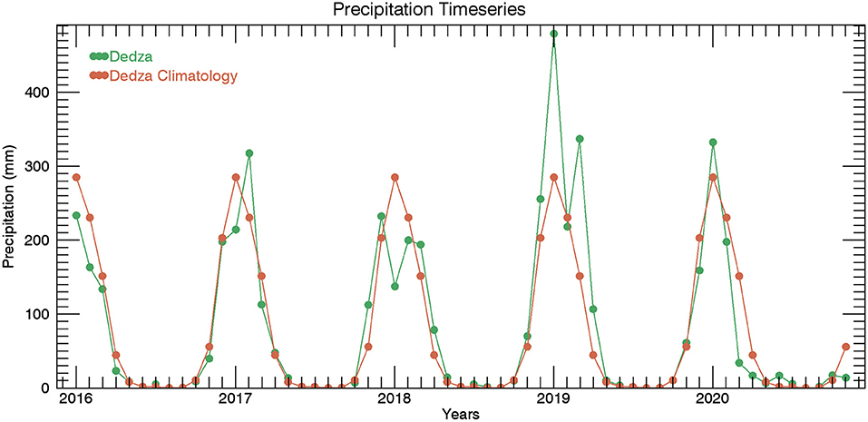
Figure 1. Precipitation (green) and average (2000–2020) monthly precipitation (orange) from CHIRPS for a 5 km pixel in an agricultural part of Dedza District, Malawi, 14.34° S, 34.13° E.

FIGURE 2

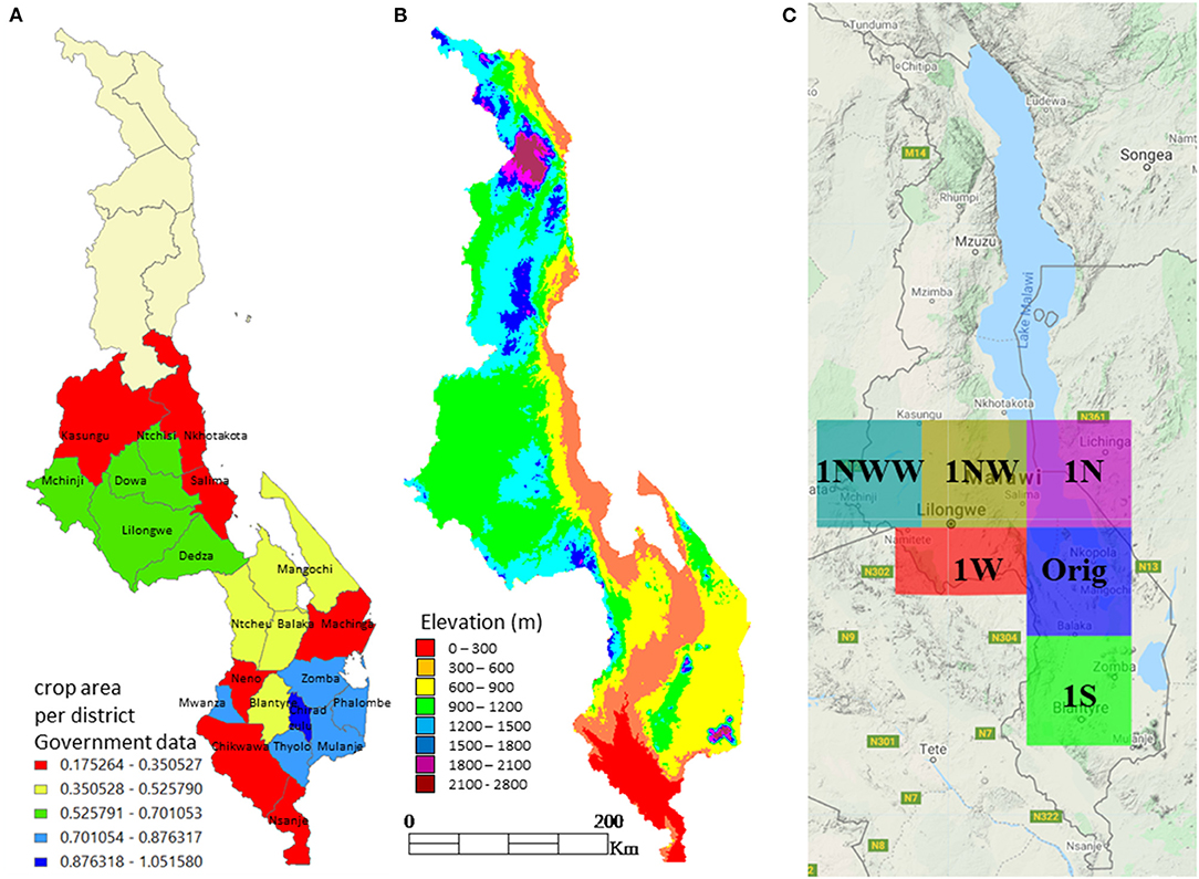
Figure 2. Study area in Malawi showing administrative districts in central and southern Malawi with fractional crop area (A), elevation for Malawi from Shuttle Radar Topography Mission (SRTM) data (B), the six initial “tiles” used to perform the Random Forest (RF) analysis, most are 1° ×1° (C).

Training Data

We divided Malawi into 1⁰ ×1⁰ tiles. This was primarily done for logistical reasons—memory restrictions in GEE. Six tiles covered the bulk of central and southern Malawi, with smaller areas added to cover the remaining portions (Figure 2). We classified the landscape into five classes: crop, open water, and three types of natural areas—sparse, shrub, forest—differentiated based on observed canopy cover. Air photo interpretation techniques were applied to very high spatial resolution (1 m pixels or less), true color imagery in Google Earth Pro (GE) to identify thousands of reference points for the crop, sparse, shrub, and forest classes, with fewer points needed for open water (Table 1). Points were identified in areas that were homogeneous over at least 20 m. The “show historical data” feature was used to examine all available imagery in GE for evidence of agricultural activity, with most imagery acquired between 2013 and 2020. Examples of different stages of agricultural activity visible in the imagery include fields plowed into regular rows, fields having regular geometric shapes, fields showing different vegetation greenness with linear distinctions—as if harvesting was in progress during image acquisition, and crop residue arranged in linear or circular patterns (Figure 3). For natural areas we sought to use imagery from 2017 or 2018 to minimize any possible landcover change effects. In contrast to agricultural areas, natural areas generally showed irregular vegetation canopies, both in terms of canopy shape and spacing between plants. They also do not show linear (man-made) features. Some manually interpreted points were able to be reused for adjacent tiles where landforms (and hence, climate/vegetation) were similar (e.g., Orig and 1N along the shore of Lake Malawi). Training data were added for each tile in an iterative process until the resulting RF classification for the tile did not contain spatially correlated errors. Points from adjacent tiles were always used to make an initial classification for a new tile to speed up the point selection process. For instance, if the initial classification map for a tile showed that forested areas were well-identified using existing training data from other tiles, no new training points were added for that class within the new tile. The reference point files were saved as KMLs and converted to shapefiles for use in GEE. Much of the effort in this research focused on the selection, interpretation, and refining of points used to drive the classification.

TABLE 1

Table 1. Training points generated in Google Earth Pro.

FIGURE 3

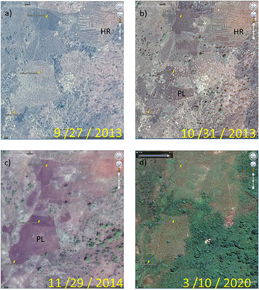
Figure 3. Four different looks in Google Earth Pro at a smallholder agriculture area in east central Malawi near 13.72°S, 35.1°E on 9/27/2013 (a), 10/31/2013 (b), 11/29/2014 (c), and 3/10/2020 (d). Harvest residue (HR) in the north east corner of the 9/27 and 10/31 images identifies this area as cropped. Plowing (PL), exposing dark, smooth soil in 11/29, and to a lesser extent 10/31 identifies this area as cropped. The fine spatial resolution allows for the identification of plant canopies in the southeast portion of the image, the temporal information suggests some of them are evergreen trees, some deciduous shrubs.

Independent Validation Data

The independent validation data used in this study came from four independent sources, the official statistics from the Government of Malawi for 2017, a map derived from interpreted satellite imagery from the USGS from 2017, the global IIASA-IFPRI crop area map from 2005 and the ESA-CCI Sentinel-2-based map from 2016. The Malawi government data consists of the area planted for each of 10–12 crop types at the district level, covering nine districts in central Malawi, and 13 in southern Malawi. The crop areas were summed and divided by the overall area of each district to get percent crop area. It should be noted that the government statistics for crop area may double count a field if it is intercropped with two different crops, hence fractions can be >1.0. The Tappan USGS map relies on expert interpretation of points on a regular 1 km grid, primarily using Landsat and Sentinel-2 data to make a determination of landcover at each point using the Rapid LandCover Mapping tool (Cotillon and Mathis, 2017). A total of 28 landcover classes were used, six of which represented agricultural areas (rainfed herbaceous crops, cultivated dambo, rice, sugar cane, tea, and tree plantation). The map was converted to binary (presence/absence) of agriculture at the 1 km pixel scale to calculate percent crop area for each district. The IIASA-IFPRI crop area map integrates existing maps from various sources, ranking and weighting them before combining them into the final global 1 km pixel crop area product (Fritz et al., 2015). The ESA-CCI map is derived from Sentinel-2 data and is available at 20 m resolution, it is unpublished and labeled as a prototype but is beginning to be evaluated in the literature (Samasse et al., 2018; Alkhalil et al., 2020).

Predictor Variables

SMA was applied to the 10 m Sentinel-2 time series for central and southern Malawi. We used the Level 1C, top of atmosphere (TOA) reflectance product rather than the Level 2A surface reflectance product, as all of the Sentinel-2 data are available in this form, allowing us an extra 2 full calendar years in analyses, because the Level 2A data are only available from mid-2017 to present while the Level 1C data begins in October 2015 in Malawi. To identify and filter out clouds, the cloudscore algorithm was used for cloud and cloud shadow masking (Chastain et al., 2019). Due to the use of top of atmosphere reflectance data, we used image EMs, derived from pure Sentinel-2 pixels of maize, senesced vegetation, and bare soil in an agricultural area in central Kenya, where we had an informant who could identify landcover, rather than reference EMs convolved to Sentinel-2 band wavelengths from hyperspectral data. Thus, atmospheric effects are included in the image EM spectra. SMA was performed on each individual Sentinel-2 image in southern and central Malawi in 2018 with the same set of EMs, breaking each pixel of each image down into its components of GV, NPV, soil, and shade. Table 2 lists the reflectance values used for each EM. For each pixel, the time series of EM fractions were summarized in two different ways: (1) the minimum, maximum, median, and range in values within each bi-monthly time step were calculated for each EM fraction (similar to the Jin et al., 2019 approach), and (2) the monthly median was calculated for each EM fraction (Kerner et al., 2020). Additionally, for each approach we calculated the annual minimum, maximum, median, and range for each EM fraction from the bimonthly/monthly medians. A threshold value of 0.4 for annual GV maximum was used to remove fields that showed evidence of agricultural activity at some point in GE imagery, but were fallow in 2018, from the crop training and test data sets. Even though these distilled datasets contain far less information than the five day repeat Sentinel-2 data, the resulting arrays of EM summary statistics were still very large, on the order of 20 GB per tile.

TABLE 2

Table 2. Sentinel-2 top of atmosphere reflectance values for the four endmembers used in this study, green vegetation (GV), non-photosynthetic vegetation (NPV), soil, and shade.

Image Classification

In order to work within the computational limitations of GEE, analysis was performed for each tile individually. The first step was to separate the reference data points for each landcover class into training and test data sets. The reference points were split roughly 50/50 into training/test for crop and shrubs, and 80/20 for the remaining, less-populous classes. It is important that the amount of training data per class is roughly equal in order to obtain an accurate map (He and Garcia, 2009). The training points were used to extract training data from the predictor variable array. We used RF to perform the classification analysis. Decision trees use a series of predictor variable splits to divide the dependent variable into more and more homogeneous groups. RF consist of an ensemble of decision trees, where trees are made to differ by changing the subsets of data used to train each tree, and allowing only a subset of the predictor variables to be evaluated at each node. The results from 500 decision trees were aggregated to produce the RF output (classified maps and contingency tables); a large number of trees is suggested to minimize error, with 500 being recommended in the literature (Probst et al., 2019). RF have been shown to perform well for this crop area classification application (Jin et al., 2019). RF were run on the training data, developing a model which was then (1) evaluated with the test data and (2) applied to the entire tile to make a map. All of the individual tile maps were then mosaicked, and crop area values for the 22 districts in central and southern Malawi were compared between our analysis, that of the Malawi Department of Agriculture, the Tappan USGS map of crop area in Malawi, the IIASA-IFPRI map, and the ESA-CCI map.

Results

The EM fraction trajectories reflect changes due to plant phenology. To highlight the separability of the different cover types, Figure 4 shows sample EM trajectories for a crop field and a natural shrubland area, located within 100 m of each other. The GV EM trajectory for the natural area follows precipitation well; green up begins in October, peak greenness occurs between January and March except for 2017, when the rainfall peak was a month late (Figure 1) and the GV peak was in April, and then there is a steady decline as the landscape dries down during the 6 months long dry season (Figure 4). Crop greenup is delayed a few months compared to shrub greenup, the timing of peak greenness is later in the season, and the peak is more pronounced than that of the natural area. Finally, there is an extended period of near zero GV values between harvest and planting the following growing season. Negative EM values, while not physically meaningful, occur because SMA is a matrix algebra transform with the constraint that fractions sum to 1.0, and can be interpreted as the absence of that EM for that time step. For this particular example the natural area demonstrated a higher GV fraction than the crop fields throughout 2018, but that is not always the case. NPV for the natural area has an inverse trend to GV, the new green leaves are dominant at the beginning of the season so NPV is low, then the leaves senesce, and woody shrub material and senesced ground cover become more exposed to the satellite, leading to an increase in NPV. A similar pattern is present during the growing season for the crop field, although it appears that harvest residue was left on the field in 2017 and 2018 as NPV remains high during the initial increase in GV for those years. The soil fractions stayed relatively consistent for the two areas in Figure 4, showing no evidence of plowing in this particular area, which is consistent with the observation, based on NPV, that harvest residue was left on the soil. Soil fraction was higher for crop areas, likely due to the presence of some exposed soil between crop rows. NPV and soil show more noise than GV, likely due to residual cloud contamination. Shade shows a similar pattern to GV as the landscape absorbs more light (high shade) when it is highly vegetated, and reflects more (low shade) when the ground is bare. Some locations experienced persistent cloud cover during parts of the rainy season, resulting in missing data in the satellite analysis and corresponding gaps in the plots shown in Figure 4.

FIGURE 4

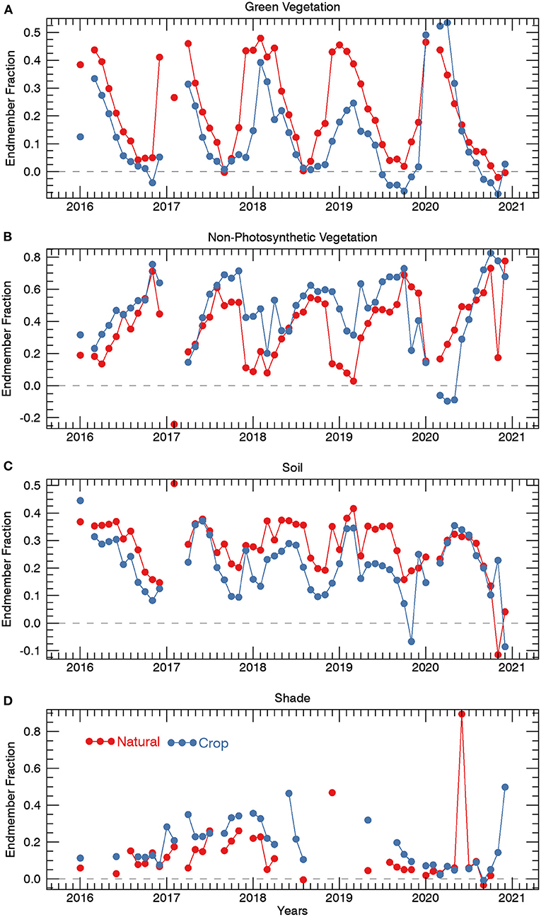
Figure 4. Sample green vegetation (GV) (A), non-photosynthetic vegetation (NPV) (B), soil (C), and shade (D) endmember (EM) trajectories for a crop area and a natural area, showing monthly median values.

We only present output for the monthly predictor variables (the second method of data distillation), as accuracies were slightly better, and the predictor variable data set was half the size of the bimonthly data set, thus it was more convenient. The overall accuracies when compared with independent test data for the six tiles with the most training data (Table 1) were on the order of 85% (Table 3). We also show data for classes re-coded to crop/no crop (Table 4), which is the more common way that crop area classifications are presented. Accuracies increased 5% for five of the six tiles, with three tiles exhibiting accuracy over 90%. Further analysis of the results in Tables 3, 4 show that the user's accuracy for crop tends to be a bit higher than the producer's accuracy, indicating a slight under-identification of agriculture in the model results, and an expected underestimate of the overall cropped area by a small amount. The biggest source of confusion was between crops and shrubs, though more crops were classified as shrub than vice versa (Table 3). It may be that the diversity in crop types and or farming intensity is more variable than shrub types, so the crop class is more heterogeneous and thus members of the class are more likely to appear to behave like shrubs.

TABLE 3

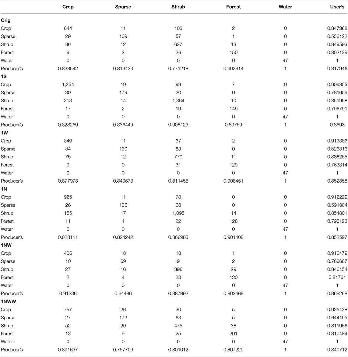
Table 3. Confusion matrices for the primary six tiles, the geographical location of the tiles is shown in Figure 2.

TABLE 4

Table 4. Confusion matrices for the primary six tiles, with the classes aggregated to crop/no crop.

Table 5 presents the variable importance values for each of the predictor variables for each of the six tiles in Table 1, with the top ten variables for each tile in bold. There are a number of interesting features. GV variables were generally most important. The median GV at the beginning of the growing season ranked high, while the median GV for the peak of the growing season (February) showed much lower importance. Natural areas green up earlier than crop areas, with separability being reduced at peak greenness (Figure 4). This also points to the advantage of monthly vs. bi-monthly variables as January and February values would have been grouped together, reducing the signal. Natural areas also remain green longer due to enhanced water availability due to established root systems, and this is reflected in high importance scores for GV variables as the season progresses. NPV showed lower importance than GV, though January was in the top ten for three tiles. January soil was also highly important. Also, soil in May, June, and July, while only in top ten importance for the NWW tile, tended to have relatively high importance. Hence, soil was important early in the growing season and during the harvest season when soil may be exposed in crop areas while natural vegetation is largely comprised of GV and NPV (Figure 4). Shade variables were second to GV in importance, with July and August being the most important months for four of the tiles. At this time of the year natural vegetation would show canopy shading due to uneven vegetation heights both within individual plants and between neighboring plants while harvested crop area would be relatively flat with higher albedo. For the remaining two tiles January was important, for similar reasons—young crops would be too small to cast much in the way of shadows compared to larger natural vegetation. The annual summary variables were generally not of high importance.

TABLE 5

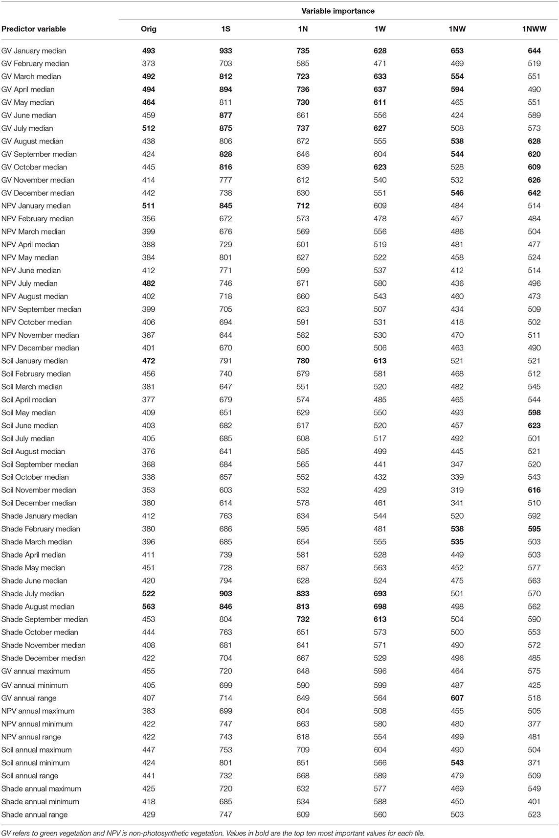
Table 5. Random Forest variable importance measures for the six primary tiles, the geographical location of the tiles is shown in Figure 2.

We mosaicked the maps from the individual tiles to generate a crop area map for all of southern and central Malawi. Seam lines were not noticeable, likely because the classification models were accurate, so there were not differences across tile boundaries. Table 6 presents crop area estimates for the different data sources. Agreement in percent crop area at the district level (comparing sets of 22 values) is high for RF, Malawi government, and Tappan USGS data sets. R² for fractional crop area at the district level between RF and Malawi government is 0.74, between RF and USGS it is 0.79, and between Malawi government and USGS it is 0.53 (Table 6). It is interesting that the relationships between RF and Malawi government and RF and USGS are similar, but the relationship between Malawi government and USGS is lower. The primary differences between the RF map and Malawi government are possible double-counted fields and human error in gathering data, both data sources cover the entire region. Both RF and USGS rely on manual image interpretation to label landcover, but RF uses all of the imagery whereas USGS examined imagery on a 1 km grid. The Malawi government data and USGS map have less in common. The ESA-CCI map shows good agreement with the RF Sentinel-2 map (R² of 0.63), however Figure 5 suggests that the ESA map systematically overpredicts crop area in southern Malawi.

TABLE 6

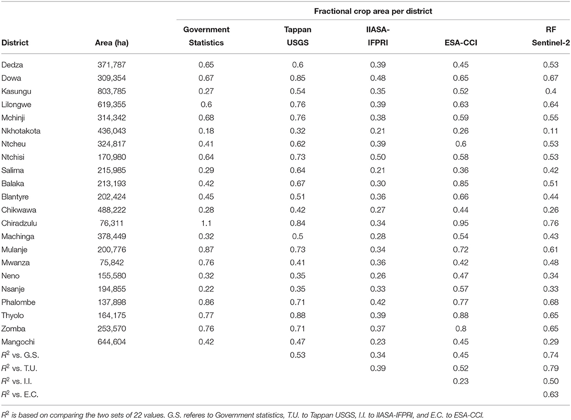
Table 6. Fractional crop area for each district in central (Dedza-Salima) and southern (Balaka-Mangochi) Malawi for the four reference data sets and the Sentinel-2 based analysis.

FIGURE 5

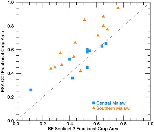
Figure 5. Fractional crop area compared for the RF Sentinel-2 map and the ESA-CCI map. The ESA-CCI map overpredicts crop area by 10–20% for many of the districts in southern Malawi.

Discussion

Our accuracies compare favorably with the three published studies examining crop area in sub-Saharan African countries at 10 m resolution that we are aware of Kerner et al. (2020), Tseng et al. (2020), and Jin et al. (2019). Kerner et al. (2020) obtained 83% accuracy when classifying crop/no crop in the country of Togo. Jin et al. (2019) obtained 85% accuracy for crop/no crop in Kenya and Tanzania. Tseng et al. obtained 86% accuracy in Kenya. However, our accuracy values are based on many more samples, making them more robust.

Aside from the increase in accuracy, the main benefit of utilizing SMA for crop area mapping is that you use the entire electromagnetic spectrum as measured by Sentinel-2, reprojected into a more intuitive/interpretable GV, NPV, soil, shade data space. Jin et al. (2019) also used a suite of greenness measures for prediction, as well as raw bands, but used additional information on vegetation structure from radar data from Sentinel-1. NPV and particularly shade can give information on vegetation structure (Roberts et al., 2002). We explored the use of Sentinel-1 data but ultimately decided against it due to some irregularities in image registration between data from the two sensors, and because of the presence of shadows/data gaps in the radar data behind taller features, due to radar being side-looking.

We chose to use TOA data rather than surface reflectance because it allows us to do temporal analyses of crop area over 5 years (2016–2020) rather than three (2018–2020). For instance, 2016 and 2017 were low rainfall years in Kenya and we could study the effect of the drought on crop area. TOA data contain atmospheric scattering that primarily affects the visible bands. For instance, for surface reflectance data, the blue band (490 nm) reflectance is usually similar to red reflectance (665 nm) for GV, whereas for TOA data there is additional blue light (Table 2). Spatio-temporal variability in atmospheric scattering should incur noise when using TOA vs. surface reflectance data, however as atmospheric scattering primarily only affects three of the ten bands it may not have had a strong effect on EM fractions, and our classification accuracies remained high. Other sources of noise include residual cloud contamination and occasional geolocation errors (particularly considering the heterogeneity of small-scale farming areas). For instance, Tremas et al. (2015) found geolocation errors for Sentinel-2 data of 12.5 m, or over 1 pixel, which could cause an agricultural area pixel to have the EM values of a neighboring forest pixel at certain timesteps, affecting monthly median and annual summary values.

Fritz et al. (2015) state that the global overall accuracy of the IIASA-IFPRI map is 82.4%, but it appears to be less accurate in Malawi, as the range in values is less than the other maps, and agreement at the district scale was low. Our finding that the IIASA-IFPRI map differed from the three other reference data sets and our classification map is in line with the findings of Samasse et al. (2018). They compared eight landcover maps in West African countries, and found that the coarser resolution maps, including IIASA-IFPRI, performed much worse than 30 m maps using Landsat data. Interestingly, the ESA-CCI 20 m map, using Sentinel-2 data, also performed worse than the Landsat-based maps with accuracies 10–40% points lower. Samasse et al. (2018) suggested the techniques and West Africa training data used in the ESA-CCI product needed to be re-examined. Alkhalil et al. (2020) also evaluated the ESA-CCI map in West Africa. They found extremely low producer's accuracies (over-prediction of crops) for three polygons in the Sahel (0.07, 0.34, 0.03) and less, but still some over-prediction for three polygons closer to the coast (producer's accuracies of 0.61, 0.72, 0.56), leading them to declare the ESA-CCI product was not an acceptable crop mask. Our research also showed overprediction of crop area by ESA-CCI when compared with the RF Sentinel-2 map, particularly in southern Malawi (Table 6, Figure 5).

RF are known as a greedy classifier, hence, a large number of manually interpreted points were identified—a total of 20,848. For comparison to other studies, central and southern Malawi comprise 6,752,347 ha. Kerner et al. (2020) mapped percent crop area in Togo (5,678,500 ha) using a different algorithm and hence, a fraction of the reference data-−1,319 crop or no crop points from within the country, and a global data set of 35,866 crop/no crop points. Tseng et al. (2020) used a similar algorithm and the same global 35,866 points, as well as 14,080 crop/no crop points for the much larger country of Kenya (58,036,700 ha). Jin et al. (2019) used RF to map crop/no crop in both Kenya and Tanzania (94,730,300 ha), 4,509 points were identified in Kenya, and 4,140 in Tanzania. The country areas are much larger than that of Malawi; however, the agricultural portion of the countries is much smaller than these numbers, making the comparison less straightforward, because large parts of each country could be excluded as potentially arable. In fact, latitude and longitude were included as predictor variables in Jin et al. (2019). Furthermore, it is not known exactly how many fewer points would have been needed if our analysis had been crop/no crop instead of crop, sparse, shrub, tree, and water. Another factor is we used roughly 50% of the data for training, 50% for testing while Jin et al. (2019) and Kerner et al. (2020) trained on 80% of the data and Tseng et al. (2020) trained on 90% of the data. Hence, they leveraged their points differently, and had fewer points for robust accuracy assessment. While our method may be less efficient and/or an excessive amount of reference points may have been identified, our accuracies are based on far more data points, which increases confidence.

This study generated a crop area map for southern and central Malawi with very high crop/no crop classification accuracies between 87 and 93%. The approach combined some of the oldest (air photo interpretation) and newest (cloud computing) remote sensing techniques. Overall, we find the results presented here to be a promising result for the potential to use GEE and RF algorithms to produce high-quality cropped area estimates for smallholder farms in rainfed agriculture regimes. EM phenology predictor variables and variable importance measures combine to produce interpretable, non-“black box” results. Accuracies for the two most populous classes, crop and shrub, are based on 50% of the reference data points so are extremely robust. A more accurate assessment of the cropped area in a region can help better understand the dynamics impacting food production and food security in vulnerable regions of sub-Saharan Africa. The method can be repeated using the same training data to perform the classification over multiple years which would be useful for the identification of changing landscape dynamics and for seasons when weather, agricultural inputs (seeds or fertilizer), or labor impacted the amount of cropped area for a particular season, over a region, relatively simply. The results presented here can also be utilized to develop an agricultural mask that can be used to better focus agroclimatic analysis over wide areas. All these different benefits could have a positive impact on the ability to anticipate, assess, and mitigate the impacts of cropped area on food security over sub-Saharan Africa.

Data Availability Statement

Publicly available datasets were analyzed in this study. This data can be found here: Publicly available Sentinel-2 data were analyzed in this study, this data can be found in Google Earth Engine.

Author Contributions

SP and GH conceptualized the research, revised, and improved the manuscript. SP defined the methods, analyzed the findings, composed the figures, and drafted the manuscript. Both authors contributed to the article and approved the submitted version.

Funding

We acknowledge support of the United States Agency for International Development (USAID) cooperative agreement #72DFFP19CA00001.

Conflict of Interest

The authors declare that the research was conducted in the absence of any commercial or financial relationships that could be construed as a potential conflict of interest.

Acknowledgments

We sincerely thank Juliet Way-Henthorne and Austin Sonnier for comments on the manuscript. Natasha Krell helped locate maize fields for determining endmember spectra. Sarah Shivers provided hyperspectral spectra of corn fields.

References

Alkhalil, A., Kadaoure, I., and Kouadio, M. (2020). An evaluation of 20-m ESA-CCI S2 prototype LC product. Front. Sustain. Food Syst. 4:504334. doi: 10.3389/fsufs.2020.504334

CrossRef Full Text | Google Scholar

Amani, M., Kakooei, M., Moghimi, A., Ghorbanian, A., Ranjar, B., Mahdavi, S., et al. (2020). Application of Google Earth Engine cloud computing platform, sentinel imagery, and neural networks for crop mapping in Canada. Remote Sens. 12:3561. doi: 10.3390/rs12213561

CrossRef Full Text | Google Scholar

Carletto, C., Jolliffe, D., and Banerjee, R. (2015). From tragedy to renaissance: improving agricultural data for better policies. J. Dev. Stud. 51, 133–148. doi: 10.1080/00220388.2014.968140

CrossRef Full Text | Google Scholar

Chastain, R., Housman, I., Goldstein, J., Finco, M., and Tenneson, K. (2019). Empirical cross sensor comparison of Sentinel-2A and 2B MSI, Landsat-8 OLI, and Landsat-7 ETM+ top of atmosphere spectral characteristics over the conterminous United States. Remote Sens. Environ. 221, 274–285. doi: 10.1016/j.rse.2018.11.012

CrossRef Full Text | Google Scholar

Chivasa, W., Mutanga, O., and Biradar, C. (2017). Application of remote sensing in estimating maize grain yield in heterogeneous African agricultural landscapes: a review. Int. J. Remote Sens. 38, 6816–6845. doi: 10.1080/01431161.2017.1365390

CrossRef Full Text | Google Scholar

Cotillon, S. E., and Mathis, M. L. (2017). Mapping Land Cover Through Time With the Rapid Land Cover Mapper—Documentation and User Manual: U.S. Geological Survey Open File Report 2017-1012. Sioux Falls, SD. doi: 10.3133/ofr20171012

CrossRef Full Text | Google Scholar

Devereux, S. (2009). Why does famine persist in Africa? Food Sec. 1, 25–35. doi: 10.1007/s,12571-008-0005-8

CrossRef Full Text | Google Scholar

ESA-CCI (2021). CCI Land Cover—S2 Prototype Land Cover 20 m Map of Africa 2016. Available online at: http://2016africalandcover20m.esrin.esa.int/ (accessed April 09, 2021).

Google Scholar

Fritz, S., See, L., McCallum, I., You, L., Bun, A., Moltchanova, E., et al. (2015). Mapping global cropland and field size. Glob. Change Biol. 21, 1980–1992. doi: 10.1111/gcb.12838

PubMed Abstract | CrossRef Full Text | Google Scholar

Funk, C. (2021). Drought, Flood, Fire: How Climate Change Contributes to Catastrophes. London: Cambridge Press. doi: 10.1017/9781108885348

CrossRef Full Text | Google Scholar

Funk, C., Peterson, P., Landsfeld, M., Pedreros, D., Verdin, J., and Shukla, S. (2015). The climate hazards infrared precipitation with stations – a new environmental record for monitoring extremes. Sci. Data 2:150066. doi: 10.1038/sdata.2015.66

PubMed Abstract | CrossRef Full Text | Google Scholar

Gorelick, N., Hancher, M., Dixon, M., Ilyushchenko, S., Thau, D., and Moore, R. (2017). Google Earth Engine: planetary-scale geospatial analysis for everyone. Remote Sens. Environ. 202, 18–27. doi: 10.1016/j.rse.2017.06.031

CrossRef Full Text | Google Scholar

Hammond, A. L. (1975). Crop forecasting from space: toward a global food watch. Science 188, 434–436. doi: 10.1126/science.188.4187.434

PubMed Abstract | CrossRef Full Text | Google Scholar

He, H., and Garcia, E. A. (2009). Learning from imbalanced data. IEEE Trans. Knowl. Data Eng. 21, 1263–1284. doi: 10.1109/TKDE.2008.239

CrossRef Full Text | Google Scholar

Huete, A. R., Liu, H. Q., Batchily, K., and van Leeuwen, W. (1997). A comparison of vegetation indices over a global set of TM images for EOS-MODIS. Remote Sens. Environ. 59, 440–451. doi: 10.1016/S0034-4257(96)00112-5

CrossRef Full Text | Google Scholar

Jin, Z., Azzari, G., You, C., Di Tommaso, S., Aston, S., Burke, M., et al. (2019). Smallholder maize area and yield mapping at national scales with Google Earth Engine. Remote Sens. Environ. 228, 115–128. doi: 10.1016/j.rse.2019.04.016

CrossRef Full Text | Google Scholar

Karlson, M., Ostwald, M., Bayala, J., Bazie, H. R., Ouedraogo, A. S., Soro, B., et al. (2020). The potential of Sentinel-2 for crop production estimation in a smallholder agroforestry landscape, Burkina Faso. Front. Environ. Sci. 8:85. doi: 10.3389/fenvs.2020.00085

CrossRef Full Text | Google Scholar

Kerner, H., Tseng, G., Becker-Reshef, I., Nakalembe, C., Barker, B., Munshell, B., et al. (2020). “Rapid response crop maps in data sparse regions,” in KDD 2020 Humanitarian Mapping Workshop, August 24, 2020 (San Diego, CA). arXiv:2006.16866v1

Google Scholar

Lobell, D. B. (2013). The use of satellite data for crop yield gap analysis. Field Crop. Res. 143, 56–64. doi: 10.1016/j.fcr.2012.08.008

CrossRef Full Text | Google Scholar

MacDonald, R. B., and Hall, F. G. (1980). Global crop forecasting. Science 208, 670–679. doi: 10.1126/science.208.4445.670

CrossRef Full Text | Google Scholar

Masiza, W., Chirima, J. G., Hamandawana, H., and Pillay, R. (2020). Enhanced mapping of smallholder crop farming landscape through image fusion and model stacking. Int. J. Remote Sens. 41, 8739–8756. doi: 10.1080/01431161.2020.1783017

CrossRef Full Text | Google Scholar

Misra, G., Cawkwell, F., and Wingler, A. (2020). Status of phenological research using Sentinel-2 data: a review. Remote Sens. 12:2760. doi: 10.3390/rs12172760

CrossRef Full Text | Google Scholar

Ozdogan, M., and Woodcock, C. E. (2006). Resolution dependent errors in remote sensing of cultivated areas. Remote Sens. Environ. 103, 203–217. doi: 10.1016/j.rse.2006.04.004

CrossRef Full Text | Google Scholar

Probst, P., Wright, M. N., and Boulesteix, A. (2019). Hyperparameters and tuning strategies for random forest. WIREs Data Mining Knowl. Discov. 9, e1301. doi: 10.1002/widm.1301

CrossRef Full Text | Google Scholar

Roberts, D. A., Numata, I., Holmes, K., Batista, G., Krug, T., Monteiro, A., et al. (2002). Large area mapping of land-cover change in Rondonia using multitemporal spectral mixture analysis and decision tree classifiers. J. Geophys. Res. 107:8073. doi: 10.1029/2001JD000374

CrossRef Full Text | Google Scholar

Rouse, J. W., Haas, R. H., Schell, J. A., and Deering, D. W. (1973). “Monitoring vegetation systems in the Great Plains with ERTS,” in Third ERTS Symposium (pp. 309–317). NASA Special Publication SP-351(1).

Google Scholar

Samasse, K., Hanan, N. P., Tappan, G., and Diallo, Y. (2018). Assessing cropland area in West Africa for agricultural yield analysis. Remote Sens. 10:1785. doi: 10.3390/rs10111785

CrossRef Full Text | Google Scholar

Tremas, T. L., Dechoz, C., Lacherade, S., Nosavan, J., and Petrucci, B. (2015). “Sentinel-2: presentation of the CAL/VAL commissioning phase,” in Proc. SPIE 9643, Image and Signal Processing for Remote Sensing XXI, 964309. doi: 10.1117/12.2194847

CrossRef Full Text | Google Scholar

Tseng, G., Kerner, H., Nakalembe, C., and Becker-Reshef, I. (2020). Annual and In-Season Mapping of Cropland at Field Scale With Sparse Labels. Tackling Climate Change with Machine Learning workshop at NeurIPS 2020. Available online at: https://www.climatechange.ai/papers/neurips2020/29/paper.pdf (accessed April 7, 2021).

Google Scholar

Verde, N., Kokkoris, I. P., Georgiadis, C., Kaimaris, D., Dimopoulos, P., Mitsopoulos, I., et al. (2020). National scale land cover classification for ecosystem services mapping and assessment, using multitemporal Copernices EO data and Google Earth Engine. Remote Sens. 12:3303. doi: 10.3390/rs12203303

CrossRef Full Text | Google Scholar

Wang, S., Di Tomasso, S., Deines, J. M., and Lobell, D. B. (2020). Mapping twenty years of corn and soybean across the US Midwest using the Landsat archive. Nat. Sci. Data 7:307. doi: 10.1038/s41597-020-00646-4

PubMed Abstract | CrossRef Full Text | Google Scholar