Estimating Remaining Carbon Budgets Using Temperature Responses Informed by CMIP6

A remaining carbon budget (RCB) estimates how much CO₂ we can emit and still reach a specific temperature target. The RCB concept is attractive since it easily communicates to the public and policymakers, but RCBs are also subject to uncertainties. The expected warming levels for a given carbon budget has a wide uncertainty range, which increases with less ambitious targets, i.e., with higher CO₂ emissions and temperatures. Leading causes of RCB uncertainty are the future non-CO₂ emissions, Earth system feedbacks, and the spread in the climate sensitivity among climate models. The latter is investigated in this paper, using a simple carbon cycle model and emulators of the temperature responses of the Earth System Models in the Coupled Model Intercomparison Project Phase 6 (CMIP6) ensemble. Driving 41 CMIP6 emulators with 127 different emission scenarios for the 21st century, we find almost perfect linear relationship between maximum global surface air temperature and cumulative carbon emissions, allowing unambiguous estimates of RCB for each CMIP6 model. The range of these estimates over the model ensemble is a measure of the uncertainty in the RCB arising from the range in climate sensitivity over this ensemble, and it is suggested that observational constraints imposed on the transient climate response in the model ensemble can reduce uncertainty in RCB estimates.

1. Introduction

The concept of remaining carbon budgets (RCBs) is appealing and highly applicable to climate mitigation policy (Zickfeld et al., 2009). It allows us to relate a specific climate target to the remaining greenhouse gases humans can release into the atmosphere and still comply with this target. However, like all simple ideas in climate science, it demonstrates ambiguities and uncertainties. Ambiguities arise as the number of specific definitions of temperature targets and RCBs increase during efforts to make concepts and procedures precise. More important, however, are the uncertainties arising from the large spread in model projections, including those of state-of-the-art climate and Earth system models (ESMs). Notably, the spread across the ensemble of models and the corresponding uncertainties in their equilibrium climate sensitivity (ECS) and RCB do not seem to diminish with increasing model complexity. The state-of-the-art versions of ESMs included in the Coupled Model Intercomparison Project Phase 6 (CMIP6) show a span in ECS of 1.6–5.6 K with 10 models out of 27 exceeding 4.5 K (Zelinka et al., 2020). The increase in ECS is primarily linked to a stronger positive cloud feedback in some of the models, although this is still under investigation. The transient climate response (TCR), defined as the mean global temperature anomaly in a 20-year period centered on year 70 in a model experiment where CO₂ concentrations increases by 1% per year, shows a span of 1.3–3.0°C in the CMIP6 experiments shown in Table 1. In the remainder of this paper these are referred to as 1% per year experiments.

TABLE 1

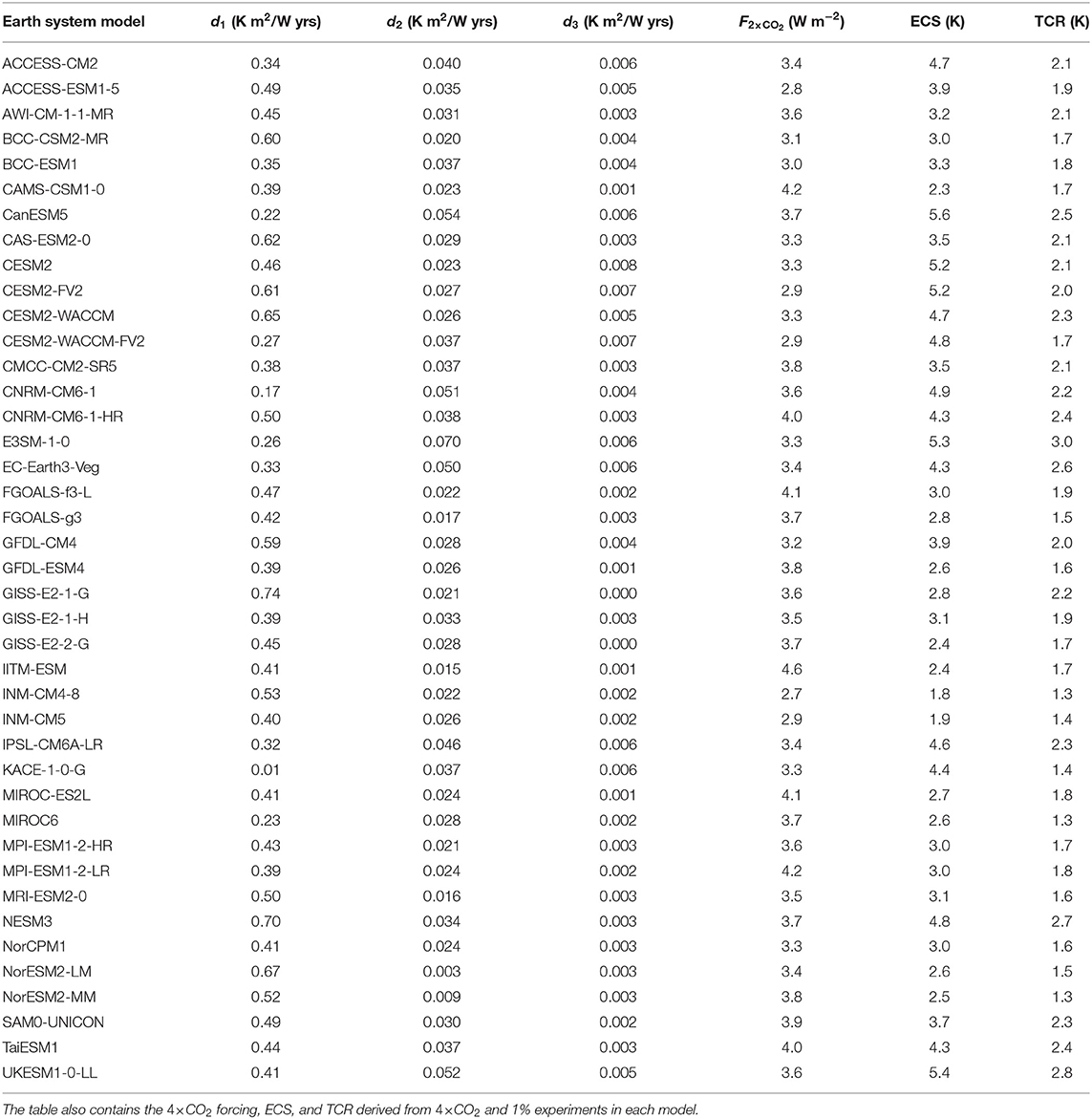
Table 1. The parameters d₁, d₂, d₃ are estimated weights for the three temperature responses with time constants 0.5, 10, 100 yrs, respectively, for the 41 CMIP6 models.

It is generally accepted that there is an approximate scenario independence in the relationship between the cumulative CO₂ emissions and the global mean surface air temperature (GSAT) over a considerable range of realistic mitigation scenarios (Allen et al., 2009; Gregory et al., 2009; Matthews et al., 2009; Meinshausen et al., 2009; Gillett et al., 2013; Goodwin et al., 2015; MacDougall and Friedlingstein, 2015; MacDougall, 2016; Rogelj et al., 2016, 2019). More precisely, there is an approximately linear relationship between the GSAT a given year and the cumulative emissions up to that year. Moreover, it turns out that in scenarios for which the emissions drop to zero at a given year, the GSAT will peak approximately that year, and hence the peak GSAT and the cumulative emissions up to the year of zero annual emissions satisfy the same linear relationship. The increase in GSAT per unit of emitted CO₂ given by this linear relation is called the transient climate response to cumulative emissions of carbon (TCRE) (Gregory et al., 2009; Stocker et al., 2013).

In this paper, we compare the cumulative emissions after 2018 in emission scenarios from the Integrated Assessment Modeling Consortium & International Institute for Applied Systems Analysis (IIASA) (Huppmann et al., 2018). Details are given in Figure 1 and Table 2. For those scenarios where annual CO₂ emissions have dropped to zero a year in this century, we compute the cumulative emissions up to that year. For those scenarios where annual emissions are still positive in year 2100, we compute the cumulative emissions up to year 2100. The corresponding GSAT values are evaluated for those years by means of a simple impulse-response model, similar to the FaIR model (Smith et al., 2018; Leach et al., 2020). A linear relationship between GSAT and cumulative emissions computed this way is estimated using linear regression, and the slope of the regression line serves as an estimate of TCRE. We define a climate target as a particular GSAT-value, e.g., 2.0°C above the pre-industrial baseline, and the estimated RCB for this target is obtained by the estimated linear relationship.

FIGURE 1

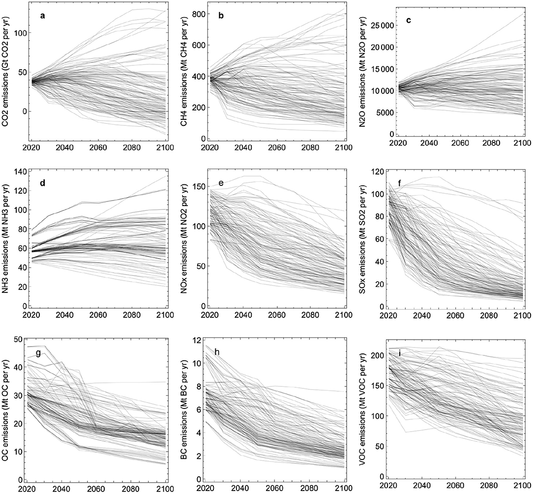
Figure 1. Emissions of greenhouse gasses and aerosols in the scenarios listed in Table 2. (a): Carbon dioxide (CO₂). (b): Methane (CH₄). (c): Nitrous oxide (N₂O). (d): Ammonia (NH₃). (e): Nitrogen oxide (NO_x). (f): Sulfur oxide (SO_x). (g): Organic carbon (OC). (h): Black carbon (BC). (i): Volatile organic compounds (VOC).

TABLE 2

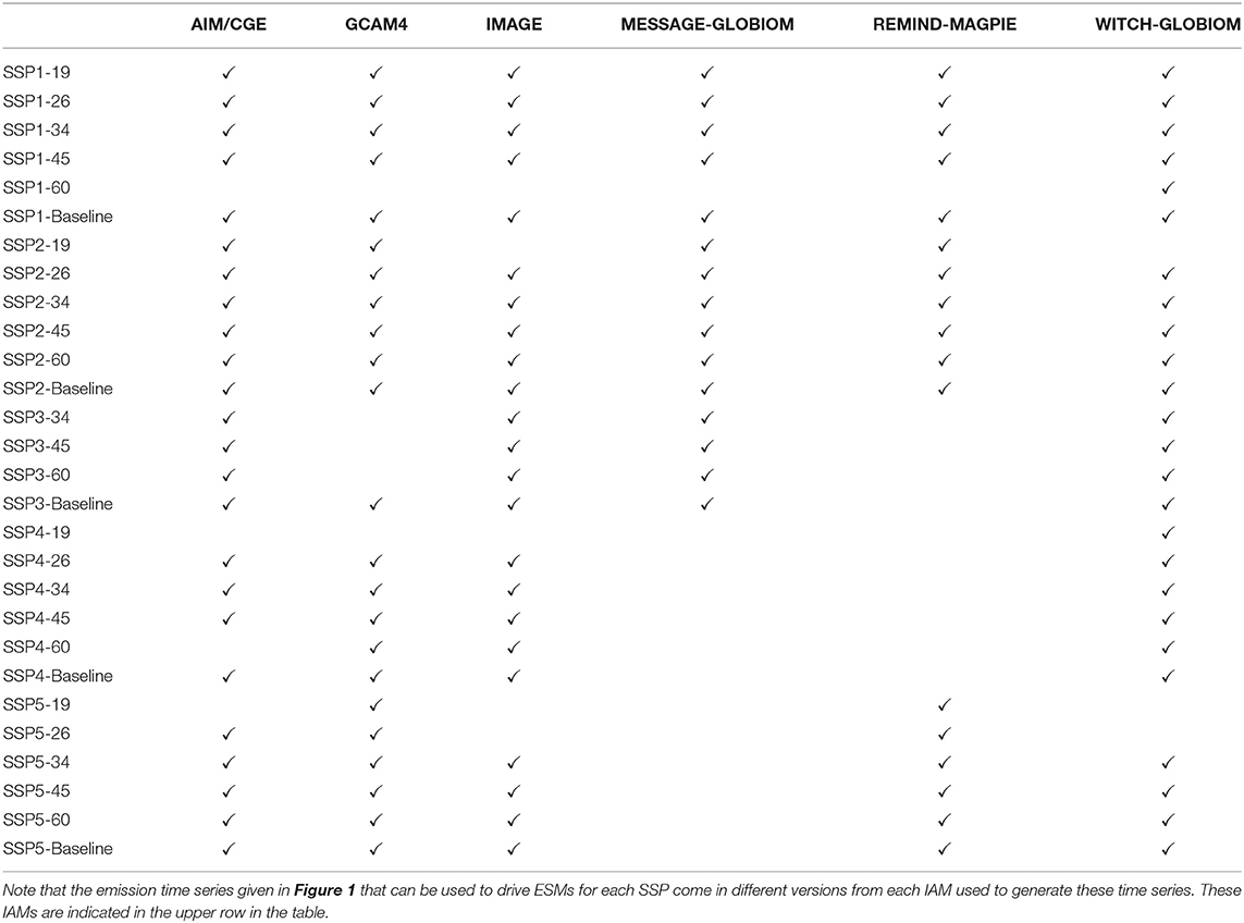
Table 2. The Shared Socioeconomic Pathways (SSPs) and integrated assessment models (IAMs) that form the 127 emission scenarios shown in Figure 1.

The transient climate response obtained by this procedure is the so-called effective transient climate response to cumulative emissions of carbon (ETCRE), since the emission scenarios contain other anthropogenic emissions than CO₂ (Matthews et al., 2017). The ETCRE includes warming from other greenhouse gases than CO₂, most importantly methane, and for cooling effects due to atmospheric aerosols. In contrast, the CO₂-only TCRE is defined as the warming attributable to CO₂ forcing alone. One can estimate the CO₂-only TCRE from ESM experiments, driven by atmospheric CO₂ concentration increases by 1% per year. The CO₂ emissions can be derived from the specified atmospheric CO₂ concentrations and the modeled atmosphere-ocean and atmosphere-land CO₂-fluxes, and hence the CO₂-only TCRE can be computed by dividing the GSAT increase by the cumulative emissions. Using 15 CMIP5 models, Gillett et al. (2013) find CO₂-only TCRE in the range 0.22−−0.65°C per 1,000 Gt CO₂, with a mean of 0.44°C per 1,000 Gt CO₂. Analyzing 11 CMIP6 models, Arora et al. (2020) found CO₂-only TCRE in the range 0.33−0.58°C per 1,000 Gt CO₂, with a mean of 0.44°C per 1,000 Gt CO₂.

The basis of these estimates are scenarios where atmospheric CO₂ concentration increases by 1% per year, and not scenarios where we reduce emissions to mitigate climate change. The reason why this does not pose a problem is the above mentioned scenario-independence of the relation between the GSAT and the cumulative emissions. The physical mechanism behind this scenario-independence is a subtle balance between a delayed warming of earlier emissions and a cooling associated with a negative forcing due to CO₂ uptake by oceans and land. If all emitted CO₂ would have remained in the atmosphere (no sinks) the warming would be delayed due to the thermal inertia of the ocean, and more so in scenarios with high emissions. However, the net CO₂ take-up by the ocean and land biosphere will increase as atmospheric concentration increases, and the ESMs indicate that the reduced CO₂ forcing due to this uptake approximately offsets the additional forcing represented by the radiation imbalance due to the delayed warming of the ocean surface. It also turns out that the warming is approximately proportional to the size of the emission increment and not strongly dependent on the background CO₂ concentration. The implication is the linear dependence of GSAT on cumulative emissions, and hence the GSAT will not increase if the emissions stop; the temperature maximum will coincide with the time the annual emissions drop to zero (Matthews et al., 2017; MacDougall et al., 2020).

There are several ways of adjusting CO₂-only TCREs and RCBs to obtain their effective counterparts. One method is to estimate the fraction of the total radiative forcing attributable to anthropogenic CO₂-emissions. In the CMIP5 ensemble, the multi-model mean ratio of CO₂ forcing to total anthropogenic forcing has been estimated to be 0.86 (Meinshausen et al., 2011; Matthews et al., 2017), which yields a multi-model mean ETCRE of 0.51°C per 1,000 Gt CO₂ based on the CO₂-only estimate of 0.44°C per 1,000 Gt CO₂ (Gillett et al., 2013).

Another approach (Matthews et al., 2017) is to estimate the ETCRE by dividing the observed 1861–2015 GSAT increase of 0.99°C by the 1870–2015 cumulative CO₂ emissions of 2,035 Gt CO₂ to obtain ETCRE = 0.49°C per 1,000 Gt CO₂. However, in ambitious yet realistic future mitigation scenarios, where emissions are brought rapidly to zero in this century, the ratio of CO₂ forcing to total anthropogenic forcing may deviate from the historical estimates. The method applied in this paper is to analyze open-source scenarios constructed using integrated assessment models (IAMs) (Huppmann et al., 2018) (Figure 1 and Table 2). In these scenarios, the total emissions of various greenhouse gasses and aerosols emissions are known, and we can obtain corresponding temperatures using a simplified version of the FaIR model (Smith et al., 2018; Leach et al., 2020). To assess the uncertainties in RCBs, one should ideally explore an ensemble of realistic mitigation scenarios using the full set of ESMs in the CMIP6 ensemble, which is not feasible due to the computational costs. In this study, we parameterize the temperature response module in our simple model by fitting those model parameters to the temperature response in two standard CO₂-forcing scenarios in each of the ESMs in the CMIP6 ensemble. Each of these simple response models emulates the corresponding temperature response to total forcing in the ESM. Combining this temperature module with the greenhouse gas and aerosol forcing module in the FaIR model we compute a temperature response to each of the emission scenarios, and the resulting GSAT time series and CO₂ emission time series in each of these model runs allows us to analyze the relationship between cumulative emissions and peak temperatures, and estimate ETCRE and RCBs. Our simple modeling set-up, described in section 2, is based on generally accepted results from the climate modeling literature, while keeping them operational and straightforward.

The philosophy of our approach has similarities to that of MacDougall et al. (2017). They emulated an ensemble of CMIP5 models by means of a climate model of intermediate complexity parameterized to have the climate sensitivity, radiative forcing, and ocean heat uptake efficiency as diagnosed from each CMIP5 model. However, their modeling framework was restricted to 1% per year experiments in the CMIP5 models which imposes carbon fluxes between the atmosphere and ocean and the atmosphere and terrestrial biosphere that may not be consistent with a fully coupled system. Apart from using a different emulator model and emulating a more recent generation of CMIP models, the main novelty in our approach is the application of the emulator model fitted to 41 CMIP6 model versions to an ensemble of 127 emission scenarios for the twenty-first century. The statistics of the estimates of ETRCE and RCB are therefore based on 5,207 distinct simulations of the emulator model.

2. Modeling Set-Up

We use a simple modeling set-up where atmospheric CO₂ concentrations are computed from the emissions, E_CO2(t), using the approach of Leach et al. (2020) which builds on Smith et al. (2018). Details are explained in those papers. The FAIR model uses anthropogenic fossil fuel and land use CO₂ emissions as input and partitions them into four pools R_i;

$\begin{array}{l}{C}_{\text{CO}{}_2}(t)=C_{\text{CO}{}_2\text{,PI}}+{\displaystyle \sum _{i=1}^4}{R}_i(t),\end{array}$

where C_CO2,PI = 280 ppm is the pre-industrial concentration. The pools represent differing time scales of carbon uptake. Here i = 1 represents uptake by geological processes, i = 2 the deep ocean, i = 3 the biosphere, and i = 4 the ocean mixed layer. The concentration in each pool varies according to the equation,

$\begin{array}{l}\frac{d{R}_i}{dt}=a_i{E}_{\text{CO}{}_2}(t)-\frac{1}{{\tau }_{\text{CO}{}_2\text{,}i}\alpha }{R}_i,\end{array}$

where E_CO2(t) is the CO₂ emission rate, a_i is the partition fraction ($\sum _{i=1}^4{a}_i=1$), and τ_CO2,iα is the characteristic time scale of the i'th pool, where the state-dependence is built into the model by letting α depend on the global temperature T(t) and the cumulative uptake G_u of agent u since initialization of the model;

$\begin{array}{l}{G}_u(t)={\displaystyle \sum _{i=1}^4\left[a_i{{{\displaystyle \int }}^{\text{}}}_{t_0}^t{E}_{\text{CO}{ }_2}(s)ds-R_i(t)\right].}\end{array}$

The time t₀ refers to the year 1750. The model for α is

$\begin{array}{l}\alpha (T,G_u)=g_{0}exp\left(\frac{r_0+r_u{G}_u+r_{T}T}{g_1}\right),\end{array}$

where r₀ is the strength of pre-industrial uptake from the atmosphere, r_u is sensitivity of uptake from atmosphere to cumulative uptake of agent since model initialization, and r_T is such sensitivity to model temperature. The parameters g₀ and g₁ are determined by a_i and τ_CO2,_i, i = 1, …, 4, and are not independent parameters. The equations determining them are given and explained in Leach et al. (2020).

We model the concentrations of methane and nitrous oxide as linear responses of scenario data for emissions:

$\begin{array}{l}{C}_{{\text{CH}}_{\text{4}}}(t)=C_{{\text{CH}}_{\text{4}},\text{ PI}}+{\displaystyle {\int }_{t_0}^t{G}_{{\text{CH}}_{\text{4}}}}(t-s)E_{{\text{CH}}_{\text{4}}}(s)ds.\end{array}$

and

$\begin{array}{l}{C}_{{\text{N}}_2\text{O}}(t)=C_{{\text{N}}_2\text{O},\text{PI}}+{\displaystyle {\int }_{t_0}^t{G}_{{\text{N}}_2\text{O}}}(t-s)E_{{\text{N}}_2\text{O}}(s)ds.\end{array}$

with $G_{\mathrm{\text{CH}}{}_4}(t)=c_{\mathrm{\text{CH}}{}_4}{e}^{-t/{\tau }_{\mathrm{\text{CH}}{}_4}}$, and similarly for N₂O. The factors c_CH4 and c_N2O are chosen to yield the current atmospheric methane and nitrous oxide concentrations based on the emissions since 1750 (Boden et al., 2017; Saunois et al., 2020). The pre-industrial concentrations are set to C_{CH4, PI} = 700 ppb and C_{N2O, PI} = 270 ppb.

The radiative forcing associated with greenhouse gas concentrations is computed using Equations (7)– (9) in Smith et al. (2018) with parameters presented in Table 3:

$\begin{array}{l}{F}_{{\text{CO}}_{\text{2}}}=[{\xi }_1{(C_{{\text{CO}}_{\text{2}}}-C_{{\text{CO}}_{\text{2}},\text{PI}})}^2+{\xi }_2|C_{{\text{CO}}_{\text{2}}}-C_{{\text{CO}}_{\text{2}},\text{PI}}|\\ +{\xi }_3(C_{{\text{N}}_2\text{O}}+C_{{\text{N}}_2\text{O},\text{PI}})+\frac{F_{\text{2}\times {\text{CO}}_{\text{2}}}}{\ln (2)})]\ln \left(\frac{C_{{\text{CO}}_{\text{2}}}}{C_{{\text{CO}}_{\text{2}},\text{PI}}}\right)\end{array}$

$\begin{array}{l}{F}_{{\text{CH}}_{\text{4}}}=\left[{\xi }_4(C_{{\text{CH}}_{\text{4}}}+C_{{\text{CH}}_{\text{4}},\text{PI}})+{\xi }_5(C_{{\text{N}}_2\text{O}}+C_{{\text{N}}_2\text{O},\text{PI}})+{\xi }_6\right]\\ \left(\sqrt{\frac{C_{{\text{CH}}_{\text{4}}}}{\mu }}-\sqrt{\frac{C_{{\text{CH}}_{\text{4}},\text{PI}}}{\mu }}\right)\end{array}$

$\begin{array}{l}{F}_{{\text{N}}_2\text{O}}=[{\xi }_7(C_{{\text{CO}}_{\text{2}}}+C_{{\text{CO}}_{\text{2}},\text{PI}})+{\xi }_8(C_{{\text{N}}_2\text{O}}+C_{{\text{N}}_2\text{O},\text{PI}})\\ +{\xi }_9(C_{{\text{CH}}_{\text{4}}}+C_{{\text{CH}}_{\text{4}},\text{PI}})+{\xi }_{10}]\left(\sqrt{\frac{C_{{\text{N}}_2\text{O}}}{\mu }}-\sqrt{\frac{C_{{\text{N}}_2\text{O},\text{PI}}}{\mu }}\right),\end{array}$

where μ = 1 ppm. The number F_2×CO2 is the forcing associated with a CO₂-doubling. This number is model-dependent and obtained from the Gregory plots for the abrupt 4×CO₂ experiments in the CMIP6 ensemble (Gregory et al., 2004). Aerosol forcing is modeled to be proportional to aerosol emissions:

$\begin{array}{l}{F}_{\text{aero}}={\gamma }_{{\text{NH}}_{\text{3}}}{E}_{{\text{NH}}_{\text{3}}}+{\gamma }_{\text{BC}}{E}_{\text{BC}}\\ +{\gamma }_{\text{OC}}{E}_{\text{OC}}+{\gamma }_{\text{NOX}}{E}_{\text{NOX}}+{\gamma }_{\text{VOC}}{E}_{\text{VOC}}\\ +{\gamma }_{\text{SOX}}{E}_{\text{SOX}}+F_{\text{aero},\text{cloud}}(E_{\text{BC}},E_{\text{OC}},E_{\text{SOX}}),\end{array}$

where the additional term

$\begin{array}{l}{F}_{\text{aero, cloud}}(E_{\text{BC}},E_{\text{OC}},E_{\text{SOX}})\\ =F_0\frac{f(E_{\text{BC}},E_{\text{OC}},E_{\text{SOX}})-f(E_{\text{BC}}^{\text{(1765)}},E_{\text{OC}}^{\text{(1765)}},E_{\text{SOX}}^{\text{(1765)}})}{f(E_{\text{BC}}^{\text{(2011)}},E_{\text{OC}}^{\text{(2011)}},E_{\text{SOX}}^{\text{(2011)}})-f(E_{\text{BC}}^{\text{(1765)}},E_{\text{OC}}^{\text{(1765)}},E_{\text{SOX}}^{\text{(1765)}})}\end{array}$

accounts for aerosol-cloud indirect effect. Here f(E_BC, E_OC, E_SOX) = β₁ ln (1 + β₂E_SOX + β₃(E_BC + E_OC)). All parameter values are listed in Table 3.

TABLE 3

Table 3. Overview of the model parameters used to compute greenhouse gas concentrations, greenhouse forcing, and aerosol forcing, following the approaches in Smith et al. (2018) and Leach et al. (2020).

Our model for the temperature response is

$\begin{array}{ll}T(t)={\displaystyle {\int }_{t_0}^t}{G}_T(t-s)F_{\text{tot}}(s)ds,& (1)\end{array}$

with F_tot = F_CO2 + F_CH4 + F_N2O + F_aero and

$\begin{array}{l}{G}_T(t)={\displaystyle \sum _{i=1}^3}{d}_i{e}^{-t/{\tau }_i}.\end{array}$

To prevent statistical overfitting we use fixed, but well-separated time scales τ_i, chosen to be 0.5, 10, and 100 yrs (Fredriksen and Rypdal, 2017). The factors d_i are estimated simultaneously from the first 150 yrs in 4 × CO₂ experiments in CMIP6, and the first 150 yrs in experiments where the CO₂ concentration is increased by 1% per yr (Figure 2). The time series are drift-adjusted using control runs of the CMIP6 models. The method for estimation is linear regression and the forcings used are F(t) = F_4×CO2 Θ(t), where Θ(t) is the unit step function, and F(t) = F_2×CO2 (ln(1.01)/ln(2))t, for the two experiments, respectively. The slow climate response, in this case the parameter d₃, is not well-constrained by 150-yr runs (Sanderson, 2020). However, the analyses in presented in this paper only concern GSAT up to the year 2100, and are insensitive to this uncertainty. Table 1 shows the estimated parameters d₁, d₂, and d₃ for the 41 models in the CMIP6 ensemble. The table also shows the TCR, ECS, and F_2×CO2 of each climate model. The ECS-values are estimated using the standard Gregory-plot technique and the TCR-values are obtained from the CMIP6 runs where CO₂ concentrations are increased by 1% per year. Using the updated HadCrut data set we set the present-day GSAT at 1.1°C above the 1850–1900 baseline (Morice et al., 2012). Historical CO₂ and methane emissions are obtained from Hoesly et al. (2018).

FIGURE 2

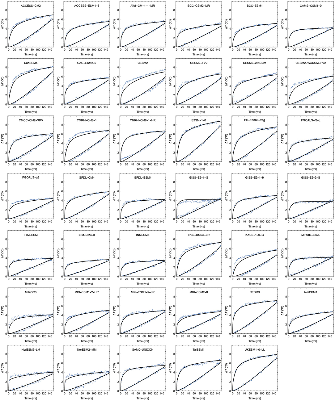
Figure 2. The points are the GSAT from the first 150 yrs in 4× CO₂ experiments and 1%-per-yr experiments in CMIP6. The solid curves are the simultaneous least-squares estimates to the two time series of a linear response to the forcings F(t) = F_{4 × CO2} Θ(t) and F(t) = F_{2 × CO2}(log(1.01)/log(2))t.

The integral in Equation (1) is computed as a discrete sum

$\begin{array}{ll}{\displaystyle \sum _{s=t_0}^t}{G}_T(t-s+\delta )F_{\text{tot}}(s)\Delta s,& (2)\end{array}$

where F_tot(s) are annual forcing values and Δs = 1 yr. We use δ = 0.5 yrs, which corresponds to the midpoint rule in the approximation of the integral. Using δ = 0 will lead to over-estimation of the temperature response compared to the exact integrals used in the parameter estimation. Figure 3 shows that δ = 0.5 yrs gives agreement between the TCRs estimated directly from the ESMs and the TCRs estimated from the discrete-time emulators.

FIGURE 3

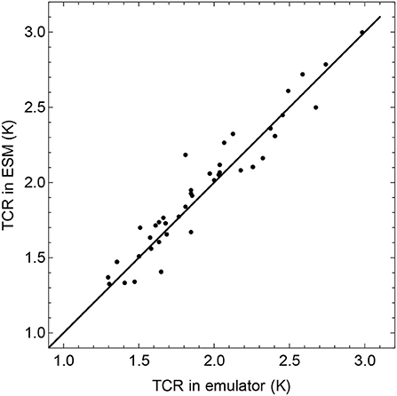
Figure 3. Comparison of TCR estimated from the 1% per year experiments in 41 ESMs and the TCR estimated in the corresponding emulators. The figure shows that the computed climate response using the discretization in Equation (2) is unbiased when using the midpoint rule, i.e., δ = 0.5 yrs.

3. Results

Our results show that the linear relationship between total emissions and maximum GSAT is an excellent approximation for each temperature-response model for cumulative emissions up to 5,000 Gt CO₂ after 2018, but that the ETCRE varies considerably over the ensemble of different temperature responses (Figure 4). Over the ensemble we find a mean ETCRE of 0.42°C per 1,000 Gt CO₂, with a 66% confidence range of 0.35–0.47°C per 1,000 Gt CO₂ (Figure 5A). Here 66% confidence range means the range between the 17 and 83% percentiles for the ensemble of 41 ETCREs estimated as the slope of the regression lines shown in Figure 4. Throughout this paper, 66% confidence range always refers to a range over a specified ensemble of models.

FIGURE 4

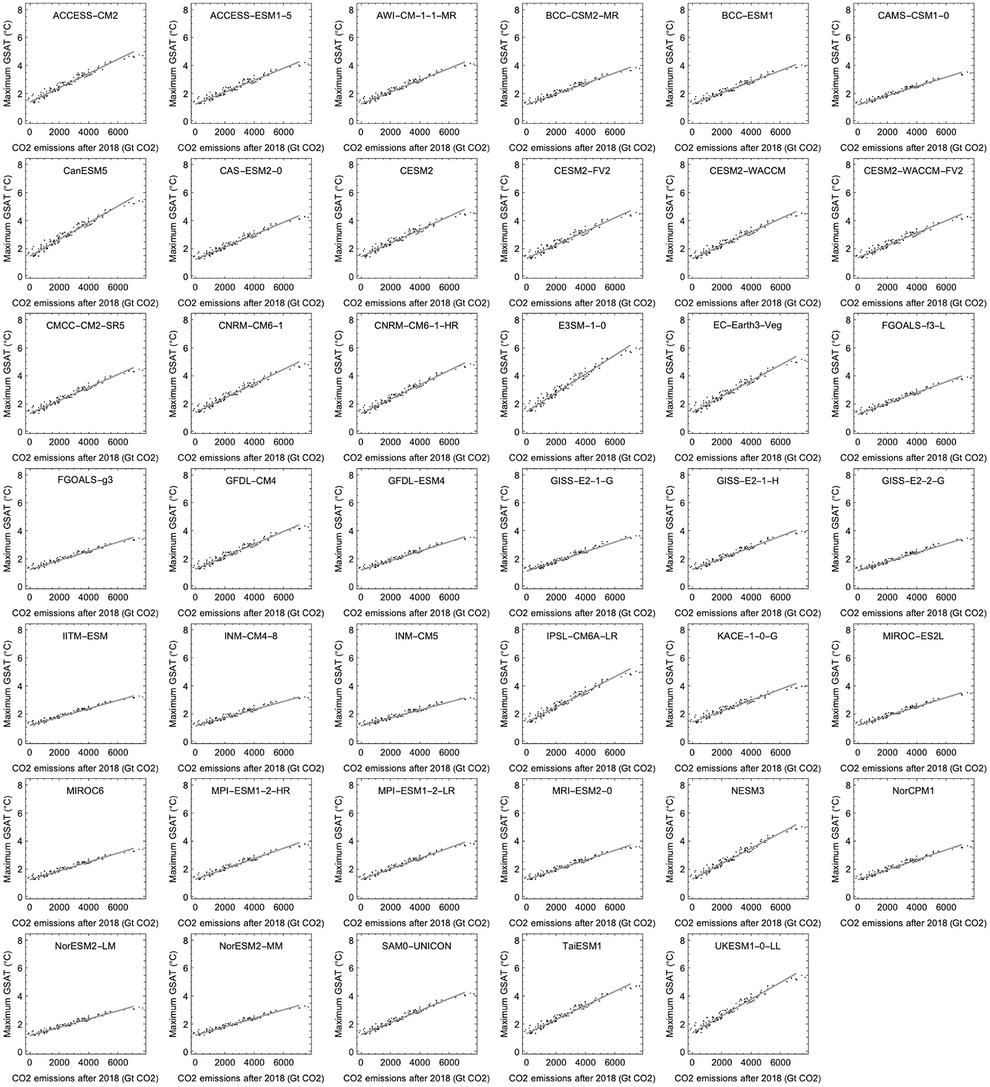
Figure 4. Estimates of ETRCE. Each panel contains 127 points representing maximum GSAT vs. cumulative CO₂ emissions obtained from our simple emulator for the indicated CMIP6 ESM, i.e., each point represents one of the 127 emission scenarios. The parameters d₁, d₂, d₃ estimated for each ESM are shown in Table 1. The regression lines demonstrate approximately linear relationships between total positive CO₂ emissions between 2018 and 2100 and the maximum GSAT for the ensemble of emission scenarios for each of the 41 different climate models in the CMIP6 ensemble. ETCRE estimates are obtained from the slopes of regression lines.

FIGURE 5

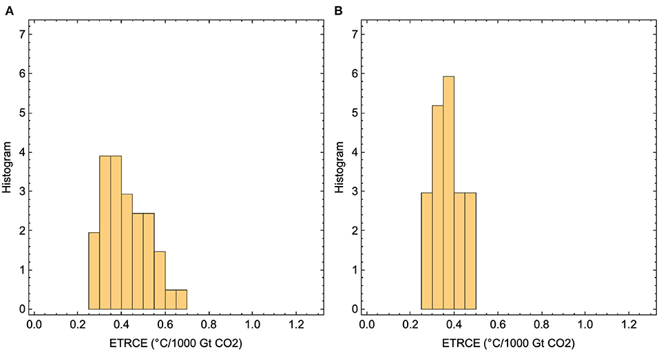
Figure 5. (A) The histogram of ETCRE-values obtained by using the full set of temperature-response models. (B) The histogram of ETCRE-values obtained using only temperature response models informed by CMIP6 models with TCR in the range 1.3–2.2 K.

Nijsse et al. (2020) have recently constrained TCR to the range 1.3–2.1 K by leaving out models with TCR≥2.2 from the ensemble. Restricting to this sub-ensemble, the 66% confidence range for ETCRE is lowered to 0.33–0.40°C per 1,000 Gt CO2 (Figure 5B).

The cumulative emissions (the RCB) for a given peak temperature target, computed for each ESM, is estimated from the regression line for that ESM in Figure 4. It allows us to construct the histograms shown in Figures 6A–D. They show how the cumulative emissions are distributed over the 41 ESMs for four different temperature targets. We note that the RCB varies by a factor of two over the model ensemble. Restricting to the sub-ensemble of models with TCR< 2.2, we find the histograms shown in Figures 6E–H. This restriction imposes a significant constraint on the lower end of the RCB range for each target, ruling out the more pessimistic estimates for the remaining carbon budget.

FIGURE 6

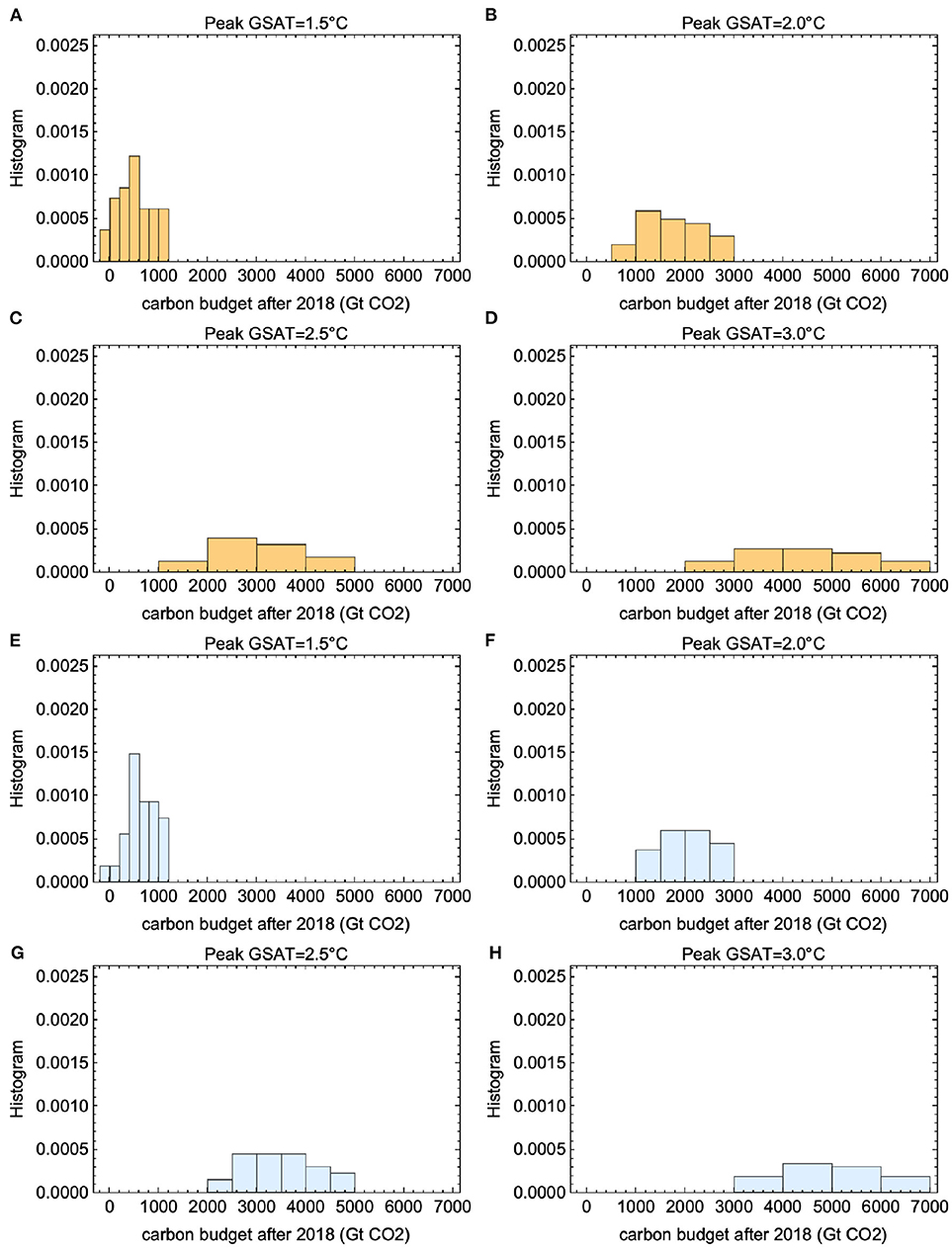
Figure 6. Estimates of RCB for different temperature targets. Panels (A–D) show histograms for the 1.5, 2.0, 2.5, and 3.0°C-targets, respectively. (E–H) The same estimates, but based only on the temperature response models informed by CMIP6 models with TCR in the range 1.3–2.2 K.

The differences in ETCRE between the high- and low-sensitivity models are illustrated in Figure 7 For the sub-ensemble of climate models with TCR ≥ 2.2 K, the mean ETCRE is 0.52°C per 1,000 Gt CO₂, with a 66% confidence range of 0.45–0.57°C per 1,000 Gt CO₂. For those climate models with TCR < 2.2 K, the mean ETCRE is 0.37°C per 1,000 Gt CO₂, with a 66% range of 0.30–0.43°C per 1,000 Gt CO₂. In Figure 8 the maximum GSAT is plotted against the cumulative CO₂ emission. This cumulative emission is different for every emission scenario, while the maximum GSAT varies across models for the same scenario. Thus, there are 127 columns of points, one for each scenario, and each point in the same column gives the GSAT for a specific model driven by that scenario. Hence, each column contains 41 points, where the blue points represents models in the TCR < 2.2 K sub-ensemble, and the red points the models in the TCR≥ 2.2 K sub-ensemble. The blue- and red-shaded areas depict the 66% ranges of GSAT in the two sub-ensembles for each scenario. We observe that the corresponding difference in RCB between the two sub-ensembles grows approximately linearly with increasing temperature target above 1.5 °C, and that model uncertainty in RCB grows linearly with the temperature target. The width of the 66% confidence range for RCB increases from 800 to 2,500 GtCO2 as the target increases from 1.5 to 3.0 °C.

FIGURE 7

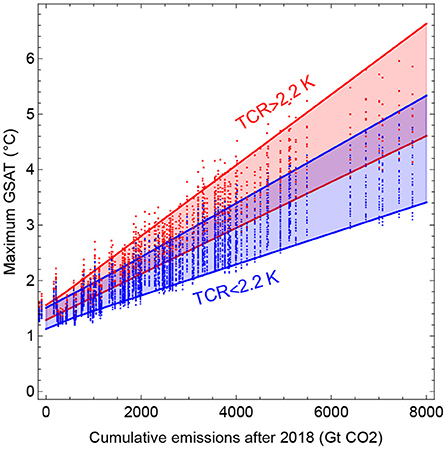
Figure 7. Each column of points shows maximum GSAT for a given emission scenario, so their spread indicates the variance over the ensemble of ESMs. The red points are for ESMs with TCR≥2.2 K, and the blue points for ESMs with TCR<2.2 K.

FIGURE 8

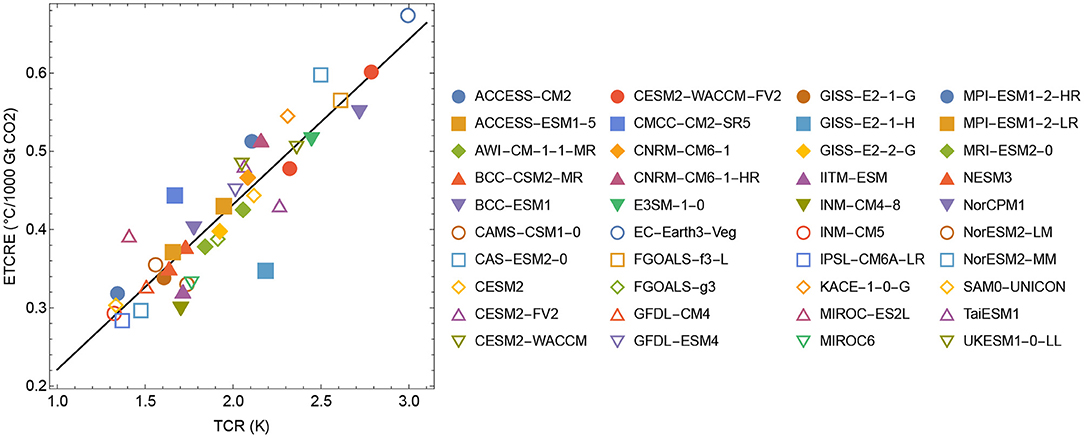
Figure 8. The approximately linear relationship between the estimated ETCRE and TCR of the CMIP6 model used to inform the temperature response model.

Figure 8 shows that the estimated ETCRE scales linearly with the TCR of the ESMs estimated from 150 yrs 1% per year experiments. The estimated relationship is

$\begin{array}{l}\text{ETCRE}=a+b\text{TCR},\end{array}$

with a = 0.21°C per 1,000 Gt CO2 and b = 0.01 per 1,000 Gt CO2. The TCR ranges from 1.3 to 3.0°C in the CMIP6 ensemble, corresponding to a range of 0.29 to 0.64°C per 1,000 Gt CO2 in ETCRE.

4. Discussion

The results shown in Figure 4 demonstrate the linearity of the maximal GSAT response to cumulative emissions over the ensemble of 127 SSP scenarios in all emulated CMIP6 models. It allows accurate estimates (small spread over the ensemble of scenarios) of the ETCRE associated with each emulated CMIP6 model. There is, however, a large spread in this model-specific ETRCE over the CMIP6 ensemble as shown in Figures 5A,B. The importance and novelty of these results are that the main uncertainty of the ETRCE and the associated RCB is not due to the spread of realistic emission scenarios, but rather the spread of sensitivities over the CMIP6 model ensemble. Figure 8 also demonstrates the close correlation between the ETRCE and the transient climate response TCR over the CMIP6 ensemble, which suggests that constraints obtained on the climate sensitivity, leading for instance to removal of hyper-sensitive models from the ensemble, will reduce the uncertainty in the estimates of the ETRCE and the RCB.

The proportionality between TCRE and TCR is not new, this was discussed in Gillett et al. (2013), and more recently in Jones and Friedlingstein (2020). It is shown in this paper, however, that it also holds for the ETCRE, i.e., as the non-CO₂ emissions are taken into account. This may not come entirely as a surprise, since studies based on the standard Representative Concentration Pathways Scenarios RCP2.6, RCP4.5, RCP6.0, and RCP8.5 show consistent dependence between non-CO₂ and CO₂ forcing throughout the twenty-first century (e.g., Williams et al., 2017). The RCPs set pathways for greenhouse gas concentrations from which the emission pathways are derived, and hence do not represent realistic socioeconomic scenarios. The SSPs, on the other hand, are based on narratives describing broad socioeconomic trends that could shape future society. These are intended to span the range of plausible futures, so we believe that the confirmation of the proportionality for this ensemble of scenarios strengthens the prospects of using the TCR to constrain TCRE and RCB.

The design of our study precludes explicit study of uncertainty due to model variation in the sensitivity of radiative forcing from CO₂ emission. This is because the parameters of module of the emulator that computes forcing from emissions are fixed and not fitted to each CMIP6 model. Our rationale for not fitting all the coefficients of the module that calculates forcing based on the input from emission scenarios is two-fold: First, we would need to have available results from at least one model run forced by such full emission scenarios for all the 41 CMIP6 models in order to make such a calibration. Second, Table 3 shows the additional 40 parameters that would be fitted to each of these model runs. Even if only a subset of the parameters were subject to fitting, the risk of statistical overfitting would be unavoidable. It seems that one is left with the choice between using a reasonably complex module with fixed coefficients for computation of forcing from emission input, or a very simple model with a few fitting parameters. In the former case, one will miss the variability among the CMIP6 models when it comes to forcing calculations. In the latter case, one may miss important mechanisms. We have chosen the former option, and unfortunately that precludes explicit evaluation of the contribution of some aspects of the CMIP6 variability to the uncertainty in RCB. Thus, the real ESM model uncertainty is probably greater than estimated in this paper, but at present, we have no means of quantifying this additional uncertainty.

The performance of the emulator model could be tested if we had available CMIP6 model runs forced by the 127 emission scenarios, or at least, by a selected few. In the CMIP6 database, we find a few runs driven by selected SSPs, but we have not been able to identify exactly the emission data input used in these runs. As more data from CMIP6 runs becomes available, we hope more comprehensive testing and refinement of the emulator will be possible.

Our analyses show that estimates of RCBs are associated with considerable uncertainty related to the global temperature response to radiative forcing, quantified for example as the spread over different members of the CMIP6 model ensemble. We further show that model estimates of ETCRE correlate strongly with TCR across models, which is convenient since much effort is being made to use observations to constrain the TCR and ECS. Cox et al. (2018) used the instrumental temperature record to constrain ECS in the CMIP5 ensemble to a 66% confidence interval of 2.2–3.4 K. This approach was based on an assumed theoretical relation between ECS and unforced temperature fluctuations, whereas the analysis reflected the forced temperature responses (Brown et al., 2018; Po-Chedley et al., 2018; Rypdal et al., 2018). To circumvent this issue, Jiménez-de-la Cuesta and Mauritsen (2019) used observational data of post 1970 warming to constrain ECS in the CMIP5 ensemble to a 95% confidence interval of 1.72–4.12 K. This result is roughly consistent with the recent results of Sherwood et al. (2020), who used multiple lines of evidence to argue that ECS above 4.5 K is unlikely. The results of this paper suggests that ruling-out the ESMs with the highest climate sensitivity would narrow the uncertainty in ETCRE. An alternative, but related, approach is to tune emulators to observational data (Smith et al., 2018). The estimated uncertainty in ETCRE corresponds directly to the uncertainty in RCB, which we find to depend linearly on the temperature target. Hence, the less ambitious the temperature target, the higher the uncertainty in the corresponding RCB.

Since we use a relatively simple carbon cycle model, there is an additional source of uncertainty that is not accounted for, induced by potentially changing feedbacks in the dynamics of the Earth system, which have been shown to be a significant source of uncertainty for RCBs (Jones and Friedlingstein, 2020). Permafrost thawing in response to rising surface temperatures leads to the release of greenhouse gases stored in high-latitude soils. The release of these additional greenhouse gases will in turn accelerate global warming.

The Amazon rainforest is another example of such a positive feedback. It has been argued and observed in climate model projections that the Amazon ecosystem might transition from its current rainforest state to a state dominated by grassland and savanna vegetation (Cox et al., 2004; Hirota et al., 2011; Lovejoy and Nobre, 2018, 2019) which would be accompanied by the release of large amounts of carbon dioxide to the atmosphere. Carbon-cycle feedbacks have an overall accelerating effect on global warming (Cox et al., 2000), and the situation seems particularly evident for the Amazon. Increasing tree mortality during a transition from rainforest to Savanna will cause the rainforest to turn from a global carbon sink to a global source of carbon (Brienen et al., 2015), as has already happened temporarily during the severe droughts of 2005 and 2010 (Feldpausch et al., 2016). Climate-change-induced dieback of the Amazon would lead to the release of additional greenhouse gases, which would further accelerate global temperature rise.

The Amazon rainforest also provides an example of how anthropogenic forcing other than greenhouse gas release can affect the climate system. Modeling evidence suggests that only partial deforestation of the Amazon rainforest might—through intricate couplings between evapotranspiration, condensational latent heating, and the South American low-level circulation system—lead to a collapse of the South American monsoon system and thus, ultimately, of the Amazon rainforest (Boers et al., 2017).

As a third example, the ice-albedo feedback implies rising temperatures in the Arctic, leading to accelerating sea ice retreat, lowering albedo, and effectively increasing mean surface temperatures regionally. This positive feedback contributes to uncertainty in ETCRE, which translates to even more considerable uncertainty in the amount of greenhouse gas emissions we can allow to still limit peak temperature to specified targets.

These three examples of positive Earth system feedbacks are all—in some form—implemented in state-of-the-art models such as the ones from the CMIP6 suite (Eyring et al., 2016), and systematic searches have revealed many abrupt transitions related to such positive feedbacks in model projections (Drijfhout et al., 2015). Nevertheless, it is still assumed that state-of-the-art models remain too stable (Valdes, 2011). The presence of positive feedbacks and potential tipping points within the Earth system adds a layer of uncertainty to RCBs that is extremely difficult to quantify.

Data Availability Statement

The original contributions presented in the study are included in the article/supplementary material, further inquiries can be directed to the corresponding author.

Author Contributions

MR, AJ, AM, EF, NB, and KR designed the study with input from all authors. K-UE, H-BF, AM, and MR processed and analyzed the CMIP6 data. MR, AJ, AM, and EF carried out the analyses. MR, NB, RG, and KR wrote the original manuscript with input from all authors, while KR wrote the revised version with input from MR.

Funding

This was TiPES contribution #66; the TiPES 399 project has received funding from the European Union's Horizon 2020 research and innovation programme under grant agreement 401 No. 820970. This work was supported by the UiT Aurora Centre Program, UiT The Arctic University of Norway (2020), and the Research Council of Norway (project number 314570). NB acknowledges funding by the Volkswagen foundation.

Conflict of Interest

The authors declare that the research was conducted in the absence of any commercial or financial relationships that could be construed as a potential conflict of interest.

References

Allen, M. R., Frame, D. J., Huntingford, C., Jones, C. D., Lowe, J. A., Meinshausen, M., et al. (2009). Warming caused by cumulative carbon emissions towards the trillionth tonne. Nature 458, 1163–1166. doi: 10.1038/nature08019

PubMed Abstract | CrossRef Full Text | Google Scholar

Arora, V. K., Katavouta, A., Williams, R. G., Jones, C. D., Brovkin, V., Friedlingstein, P., et al. (2020). Carbon-concentration and carbon-climate feedbacks in CMIP6 models and their comparison to CMIP5 models. Biogeosciences 17, 4173–4222. doi: 10.5194/bg-17-4173-2020

CrossRef Full Text | Google Scholar

Boden, T., Marland, G., and Andres, R. J. (2017). Global, Regional, and National Fossil-Fuel Co2 Emissions (1751 - 2014). Carbon Dioxide Information Analysis Center (CDIAC), Oak Ridge National Laboratory (ORNL).

Google Scholar

Boers, N., Marwan, N., Barbosa, H. M. J., and Kurths, J. (2017). A deforestation-induced tipping point for the south American monsoon system. Sci. Rep. 7:41489. doi: 10.1038/srep41489

PubMed Abstract | CrossRef Full Text | Google Scholar

Brienen, R. J. W., Phillips, O. L., Feldpausch, T. R., Gloor, E., Baker, T. R., Lloyd, J., et al. (2015). Long-term decline of the amazon carbon sink. Nature 519, 344–348. doi: 10.1038/nature14283

PubMed Abstract | CrossRef Full Text | Google Scholar

Brown, P. T., Stolpe, M. B., and Caldeira, K. (2018). Assumptions for emergent constraints. Nature 563, E1–E3. doi: 10.1038/s41586-018-0638-5

CrossRef Full Text | Google Scholar

Cox, P. M., Betts, R. A., Collins, M., Harris, P. P., Huntingford, C., and Jones, C. D. (2004). Amazonian forest dieback under climate-carbon cycle projections for the 21st century. Theoret. Appl. Climatol. 78, 137–156. doi: 10.1007/s00704-004-0049-4

CrossRef Full Text | Google Scholar

Cox, P. M., Betts, R. A., Jones, C. D., Spall, S. A., and Totterdell, I. J. (2000). Acceleration of global warming due to carbon-cycle feedbacks in a coupled climate model. Nature 408, 184–187. doi: 10.1038/35041539

PubMed Abstract | CrossRef Full Text | Google Scholar

Cox, P. M., Huntingford, C., and Williamson, M. S. (2018). Emergent constraint on equilibrium climate sensitivity from global temperature variability. Nature 553, 319–322. doi: 10.1038/nature25450

PubMed Abstract | CrossRef Full Text | Google Scholar

Drijfhout, S., Bathiany, S., Beaulieu, C., Brovkin, V., Claussen, M., Huntingford, C., et al. (2015). Catalogue of abrupt shifts in intergovernmental panel on climate change climate models. Proc. Natl. Acad. Sci. U.S.A. 112, E5777–E5786. doi: 10.1073/pnas.1511451112

PubMed Abstract | CrossRef Full Text | Google Scholar

Eyring, V., Bony, S., Meehl, G. A., Senior, C. A., Stevens, B., Stouffer, R. J., et al. (2016). Overview of the coupled model intercomparison project phase 6 (CMIP6) experimental design and organization. Geosci. Model Dev. 9, 1937–1958. doi: 10.5194/gmd-9-1937-2016

CrossRef Full Text | Google Scholar

Feldpausch, T. R., Phillips, O. L., Brienen, R. J. W., Gloor, E., Lloyd, J., Lopez-Gonzalez, G., et al. (2016). Amazon forest response to repeated droughts. Glob. Biogeochem. Cycles 30, 964–982. doi: 10.1002/2015GB005133

CrossRef Full Text | Google Scholar

Fredriksen, H.-B., and Rypdal, M. (2017). Long-range persistence in global surface temperatures explained by linear multibox energy balance models. J. Clim. 30, 7157–7168. doi: 10.1175/JCLI-D-16-0877.1

CrossRef Full Text | Google Scholar

Gillett, N. P., Arora, V. K., Matthews, D., and Allen, M. R. (2013). Constraining the ratio of global warming to cumulative CO2 emissions using CMIP5 simulations*. J. Clim. 26, 6844–6858. doi: 10.1175/JCLI-D-12-00476.1

CrossRef Full Text | Google Scholar

Goodwin, P., Williams, R. G., and Ridgwell, A. (2015). Sensitivity of climate to cumulative carbon emissions due to compensation of ocean heat and carbon uptake. Nat. Geosci. 8, 29–34. doi: 10.1038/ngeo2304

CrossRef Full Text | Google Scholar

Gregory, J. M., Ingram, W. J., Palmer, M. A., Jones, G. S., Stott, P. A., Thorpe, R. B., et al. (2004). A new method for diagnosing radiative forcing and climate sensitivity. Geophys. Res. Lett. 31:L03205. doi: 10.1029/2003GL018747

CrossRef Full Text | Google Scholar

Gregory, J. M., Jones, C. D., Cadule, P., and Friedlingstein, P. (2009). Quantifying carbon cycle feedbacks. J. Clim. 22, 5232–5250. doi: 10.1175/2009JCLI2949.1

CrossRef Full Text | Google Scholar

Hirota, M., Holmgren, M., Van Nes, E. H., and Scheffer, M. (2011). Global resilience of tropical forest and savanna to critical transitions. Science 334, 232–235. doi: 10.1126/science.1210657

PubMed Abstract | CrossRef Full Text | Google Scholar

Hoesly, R. M., Smith, S. J., Feng, L., Klimont, Z., Janssens-Maenhout, G., Pitkanen, T., et al. (2018). Historical (1750-2014) anthropogenic emissions of reactive gases and aerosols from the community emissions data system (CEDS). Geosci. Model Dev. 11, 369–408. doi: 10.5194/gmd-11-369-2018

CrossRef Full Text | Google Scholar

Huppmann, D., Kriegler, E., Krey, V., Riahi, K., Rogelj, J., Calvin, K., et al. (2018). IAMC 1.5°C Scenario Explorer and Data Hosted by IIASA. Geneva: Intergovernmental Panel on Climate Change.

Google Scholar

Jiménez-de-la Cuesta, D., and Mauritsen, T. (2019). Emergent constraints on earth's transient and equilibrium response to doubled Co2 from post-1970s global warming. Nat. Geosci. 12, 902–905. doi: 10.1038/s41561-019-0463-y

CrossRef Full Text | Google Scholar

Jones, C. D., and Friedlingstein, P. (2020). Quantifying process-level uncertainty contributions to TCRE and carbon budgets for meeting paris agreement climate targets. Environ. Res. Lett. 15:074019. doi: 10.1088/1748-9326/ab858a

CrossRef Full Text | Google Scholar

Leach, N. J., Jenkins, S., Nicholls, Z., Smith, C. J., Lynch, J., Cain, M., et al. (2020). Fairv2.0.0: a generalised impulse-response model for climate uncertainty and future scenario exploration. Geosci. Model Dev. Discuss. 2020, 1–48. doi: 10.5194/gmd-14-3007-2021

CrossRef Full Text | Google Scholar

Lovejoy, T. E., and Nobre, C. (2018). Amazon tipping point. Sci. Adv. 4:eaat2340. doi: 10.1126/sciadv.aat2340

CrossRef Full Text | Google Scholar

Lovejoy, T. E., and Nobre, C. (2019). Amazon tipping point: last chance for action. Sci. Adv. 5:eaba2949. doi: 10.1126/sciadv.aba2949

PubMed Abstract | CrossRef Full Text | Google Scholar

MacDougall, A. H. (2016). The transient response to cumulative Co2 emissions: a review. Curr. Clim. Change Rep. 2, 39–47. doi: 10.1007/s40641-015-0030-6

CrossRef Full Text | Google Scholar

MacDougall, A. H., and Friedlingstein, P. (2015). The origin and limits of the near proportionality between climate warming and cumulative CO2 emissions. J. Clim. 28, 4217–4230. doi: 10.1175/JCLI-D-14-00036.1

CrossRef Full Text | Google Scholar

MacDougall, A. H., Frölicher, T. L., Jones, C. D., Rogelj, J., Matthews, H. D., Zickfeld, K., et al. (2020). Is there warming in the pipeline? A multi-model analysis of the zero emissions commitment from Co2. Biogeosciences 17, 2987–3016. doi: 10.5194/bg-17-2987-2020

CrossRef Full Text | Google Scholar

MacDougall, A. H., Swart, N. C., and Knutti, R. (2017). The uncertainty in the transient climate response to cumulative Co2 emissions arising from the uncertainty in physical climate parameters. J. Clim. 30, 813–827. doi: 10.1175/JCLI-D-16-0205.1

CrossRef Full Text | Google Scholar

Matthews, H. D., Gillett, N. P., Stott, P. A., and Zickfeld, K. (2009). The proportionality of global warming to cumulative carbon emissions. Nature 459, 829–832. doi: 10.1038/nature08047

PubMed Abstract | CrossRef Full Text | Google Scholar

Matthews, H. D., Landry, J.-S., Partanen, A.-I., Allen, M., Eby, M., Forster, P. M., et al. (2017). Estimating carbon budgets for ambitious climate targets. Curr. Clim. Change Rep. 3, 69–77. doi: 10.1007/s40641-017-0055-0

CrossRef Full Text | Google Scholar

Meinshausen, M., Meinshausen, N., Hare, W., Raper, S. C. B., Frieler, K., Knutti, R., et al. (2009). Greenhouse-gas emission targets for limiting global warming to 2 °c. Nature 458, 1158–1162. doi: 10.1038/nature08017

PubMed Abstract | CrossRef Full Text | Google Scholar

Meinshausen, M., Smith, S. J., Calvin, K., Daniel, J. S., Kainuma, M. L. T., Lamarque, J. F., et al. (2011). The RCP greenhouse gas concentrations and their extensions from 1765 to 2300. Clim. Change 109:213. doi: 10.1007/s10584-011-0156-z

CrossRef Full Text | Google Scholar

Morice, C. P., Kennedy, J. J., Rayner, N. A., and Jones, P. D. (2012). Quantifying uncertainties in global and regional temperature change using an ensemble of observational estimates: the HadCRUT4 data set. J. Geophys. Res. Atmos. 117:D08101. doi: 10.1029/2011JD017187

CrossRef Full Text | Google Scholar

Nijsse, F. J. M. M., Cox, P. M., and Williamson, M. S. (2020). Emergent constraints on transient climate response (TCR) and equilibrium climate sensitivity (ECS) from historical warming in CMIP5 and CMIP6 models. Earth Syst. Dyn. 11, 737–750. doi: 10.5194/esd-11-737-2020

CrossRef Full Text | Google Scholar

Po-Chedley, S., Proistosescu, C., Armour, K. C., and Santer, B. D. (2018). Climate constraint reflects forced signal. Nature 563, E6–E9. doi: 10.1038/s41586-018-0640-y

PubMed Abstract | CrossRef Full Text | Google Scholar

Rogelj, J., Forster, P. M., Kriegler, E., Smith, C. J., and Séférian, R. (2019). Estimating and tracking the remaining carbon budget for stringent climate targets. Nature 571, 335–342. doi: 10.1038/s41586-019-1368-z

PubMed Abstract | CrossRef Full Text | Google Scholar

Rogelj, J., Schaeffer, M., Friedlingstein, P., Gillett, N. P., van Vuuren, D. P., Riahi, K., et al. (2016). Differences between carbon budget estimates unravelled. Nat. Clim. Change 6:245. doi: 10.1038/nclimate2868

CrossRef Full Text | Google Scholar

Rypdal, M., Fredriksen, H.-B., Rypdal, K., and Steene, R. J. (2018). Emergent constraints on climate sensitivity. Nature 563, E4–E5. doi: 10.1038/s41586-018-0639-4

CrossRef Full Text | Google Scholar

Sanderson, B. (2020). Relating climate sensitivity indices to projection uncertainty. Earth System Dyn. 11, 721–735. doi: 10.5194/esd-11-721-2020

CrossRef Full Text | Google Scholar

Saunois, M., Stavert, A. R., Poulter, B., Bousquet, P., Canadell, J. G., Jackson, R. B., et al. (2020). The global methane budget 2000-2017. Earth Syst. Sci. Data 12, 1561–1623. doi: 10.5194/essd-12-1561-2020

CrossRef Full Text | Google Scholar

Sherwood, S., Webb, M. J, Annan, J. D., Armour, K. C., Forster, P.M., Hargreaves, J. C., et al. (2020). An assessment of earth's climate sensitivity using multiple lines of evidence. Rev. Geophys. 58:e2019RG000678. doi: 10.1029/2019RG000678

PubMed Abstract | CrossRef Full Text | Google Scholar

Smith, C. J., Forster, P. M., Allen, M., Leach, N., Millar, R. J., Passerello, G. A., et al. (2018). Fair v1.3: a simple emissions-based impulse response and carbon cycle model. Geosci. Model Dev. 11, 2273–2297. doi: 10.5194/gmd-11-2273-2018

CrossRef Full Text | Google Scholar

Stocker, T., Qin, D., Plattner, G.-K., Alexander, L., Allen, S., Bindoff, N., et al. (2013). Technical Summary. Cambridge, UK; New York, NY: Cambridge University Press.

Google Scholar

Valdes, P. (2011). Built for stability. Nat. Geosci. 4, 414–416. doi: 10.1038/ngeo1200

CrossRef Full Text | Google Scholar

Williams, R. G., Roussenov, V., Goodwin, P., Resplandy, L., and Bopp, L. (2017). Sensitivity of global warming to carbon emissions: effects of heat and carbon uptake in a suite of earth system models. J. Clim. 30, 9343–9363. doi: 10.1175/JCLI-D-16-0468.1

CrossRef Full Text | Google Scholar

Zelinka, M. D, Myers, T. A., McCoy, D. T., Po-Chedley, S., Caldwell, P.M., Ceppi, P., et al. (2020). Causes of higher climate sensitivity in CMIP6 models. Geophys. Res. Lett. 47:e2019GL085782. doi: 10.1029/2019GL085782

CrossRef Full Text | Google Scholar

Zickfeld, K., Eby, M., Matthews, H. D., and Weaver, A. J. (2009). Setting cumulative emissions targets to reduce the risk of dangerous climate change. Proc. Natl. Acad. Sci. U.S.A. 106, 16129–16134. doi: 10.1073/pnas.0805800106

PubMed Abstract | CrossRef Full Text | Google Scholar