Estimation of Return Levels for Extreme Skew Surge Coastal Flooding Events in the Delaware and Chesapeake Bays for 1980–2019

Extreme storm surges can overwhelm many coastal flooding protection measures in place and cause severe damages to private communities, public infrastructure, and natural ecosystems. In the US Mid-Atlantic, a highly developed and commercially active region, coastal flooding is one of the most significant natural hazards and a year-round threat from both tropical and extra-tropical cyclones. Mean sea levels and high-tide flood frequency has increased significantly in recent years, and major storms are projected to increase into the foreseeable future. We estimate extreme surges using hourly water level data and harmonic analysis for 1980–2019 at 12 NOAA tide gauges in and around the Delaware and Chesapeake Bays. Return levels (RLs) are computed for 1.1, 3, 5, 10, 25, 50, and 100-year return periods using stationary extreme value analysis on detrended skew surges. Two traditional approaches are investigated, Block Maxima fit to General Extreme Value distribution and Points-Over-Threshold fit to Generalized Pareto distribution, although with two important enhancements. First, the GEV r-largest order statistics distribution is used; a modified version of the GEV distribution that allows for multiple maximum values per year. Second, a systematic procedure is used to select the optimum value for r (for the BM/GEVr approach) and the threshold (for the POT/GP approach) at each tide gauge separately. RLs have similar magnitudes and spatial patterns from both methods, with BM/GEVr resulting in generally larger 100-year and smaller 1.1-year RLs. Maximum values are found at the Lewes (Delaware Bay) and Sewells Point (Chesapeake Bay) tide gauges, both located in the southwest region of their respective bays. Minimum values are found toward the central bay regions. In the Delaware Bay, the POT/GP approach is consistent and results in narrower uncertainty bands whereas the results are mixed for the Chesapeake. Results from this study aim to increase reliability of projections of extreme water levels due to extreme storms and ultimately help in long-term planning of mitigation and implementation of adaptation measures.

Introduction

Coastal flooding poses the greatest threat to human life and is often the source of much of the damage resulting from the storm surge and waves of coastal weather systems (Blake and Gibney, 2011; Rappaport, 2014; Chippy and Jawahar, 2018; Weinkle et al., 2018). Relative sea-level rise (SLR) rates and high-tide flooding frequency and magnitude along the US East Coast have increased in recent decades and are expected to continue increasing into the near future (Sweet et al., 2017a, 2018; Oppenheimer et al., 2019) with recent studies estimating mean sea levels are rising faster than predicted (Grinsted and Christensen, 2021). The US Mid-Atlantic coast is noted for especially high SLR rates (Sallenger et al., 2012; Kopp, 2013; Boon et al., 2018; Piecuch et al., 2018) and states and counties in this region view coastal flooding as one of their most severe and pervasive natural hazards to prepare for (Callahan et al., 2017; Boesch et al., 2018; Dupigny-Giroux et al., 2018). Increases in sea levels lead directly to higher frequencies of coastal flooding from high tides as well as minor and major coastal storms (Lin et al., 2016; Dahl et al., 2017; Garner et al., 2017; Rahmstorf, 2017; Sweet et al., 2017b; Muis et al., 2020; Taherkhani et al., 2020).

Many of the largest coastal flooding events along the US Mid-Atlantic coast are caused by tropical cyclones (TCs), most notably Hurricanes Isabel in 2003 and Sandy in 2012. For both the US Atlantic and Gulf Coasts, tropical cyclones are the costliest and most damaging weather and climate events (Smith, 2021). Under current global warming scenarios, atmospheric water vapor content and sea-surface temperatures (SSTs) in the North Atlantic Ocean are projected to increase, leading to an increase in the number of severe tropical cyclones, decreases in the forward translational speed, increases in wind speed, and increases in the rate of intensification, especially near the coasts (Kossin et al., 2017; Kossin, 2018; Knutson et al., 2019, 2020; Murakami et al., 2020; Yang et al., 2020; Wang and Toumi, 2021).

Although TCs may gather much of the attention, the threat of major coastal flooding in the region is year-round (Dupigny-Giroux et al., 2018). TCs can account for 40–60% of the top 10 flood events with higher relative percentages in the southern part of the region (Booth et al., 2016; Callahan et al., 2021b), however, the great majority of all coastal flood events, ~85–90%, in the Mid-Atlantic come from non-tropical weather systems (Callahan et al., 2021b). East Coast winter storms, surface high pressure systems, extratropical cyclones (ETCs), and frontal systems regularly impact the region throughout the year (Hirsch et al., 2001; Thompson et al., 2013). ETCs in the Mid-Atlantic in the winter and spring are often dictated by the relative position of troughs in the westerly polar jet stream, directing low-pressure systems to travel northeastward up the coast over warmer waters, often intensifying into strong nor-Easter storms. The intensity and winds of ETCs, as well as associated beach erosion and other damages due to coastal flooding, are also projected to increase due to climate change, however projections of ETC storm tracks and landfalling TCs due to changing synoptic atmospheric patterns (i.e., “storminess”) in the Mid-Atlantic is inconclusive (Hall et al., 2016; Mawdsley and Haigh, 2016; Dupigny-Giroux et al., 2018). Studies have found that US East Coast sea levels vary with synoptic oscillations (Colle et al., 2015; Wahl and Chambers, 2015; Sweet et al., 2020), leading, Rashid Md et al. (2019) to conclude that interannual and multi-decadal variability of extreme storm surge in the Mid-Atlantic was in a transition zone between more clear relationships found in the Northeast and Southeast portions of the US Atlantic Coast.

Water levels in the Delaware and Chesapeake Bays, two of the largest estuaries in the US located in the Mid-Atlantic, have been well monitored for several decades by high-quality tide-gauge networks, well-suited for climate studies (Holgate et al., 2013; Sweet et al., 2017a; NOAA NWLON, 2020; NOAA PORTS, 2020). This highly developed, economically critical region includes many commercial industries, vast amounts of public and private infrastructure, and provides important ecosystem services (Sanchez et al., 2012; Partnership for the Delaware Estuary (PDE), 2017; Chesapeake Bay Program, 2020). Impacts and costs associated with coastal flooding are highly dependent upon both the natural and social vulnerability, the amount of exposure, and adaptation measures in place (Hallegatte et al., 2013; Hinkel et al., 2014). Extreme coastal flooding can overwhelm protections in place and can have profound negative effects in this region, such as saltwater intrusion, loss of wetland forests and low-lying agricultural fields, beach erosion, damage to infrastructure from surge and waves, and flooding of roads and personal property putting human life at risk. Extreme events often include multiple hazards that compound the damage, leading to their net impact to be greater than the sum of its parts (Kopp et al., 2017; Moftakhari et al., 2017).

Estimating frequency and severity of extreme coastal flooding is difficult as, by definition, these events do not occur often. This lack of observational data makes it difficult to develop robust statistical or physical predictive models at the usual level of confidence although planning and design for extremes are essential to avoid the most severe consequences (Walton, 2000; Calafat and Marcos, 2020). Numerous hazard/risk assessments and flood insurance premiums rely on the FEMA 100-year (i.e., 1% annual chance) base flood elevations. However, many local decisions on infrastructure development, major capital investments, and adaptation planning require estimates of extreme flood levels at shorter-term return periods. Construction and maintenance of paved surfaces (10–20 years) and major roadways and bridges (50–70 years or more) for transportation as well as for wastewater treatment plants, residential development, dams/levees, beach replenishment, and wetland restoration are examples of projects in the region that require estimates of return level probabilities at time periods <100 years (DNREC, 2012; Johnson, 2013; Callahan et al., 2017; Delaware Emergency Management Agency (DEMA), 2018).

A common method to estimate the frequency of extremes (i.e., extreme value analysis, or EVA) is by assuming the largest values from an observational record can be modeled by a statistical distribution distinct from the parent distribution. Two families of extreme value distributions have been shown to model extreme values well: the generalized extreme value (GEV) distribution and the Generalized Pareto (GP) distribution (Coles, 2001). The GEV distribution can be fit to the set of maximum values of discrete, non-overlapping blocks within a time series, such as annual maximum values; this is termed the Block Maxima (BM) approach. Data points using this approach are evenly distributed over time, however, non-extreme data points from years with abnormally low values may be forced into the model fit, biasing the results. In contrast, the GP distribution can be fit to the upper tail of the parent distribution, i.e., the set of values that are greater than a pre-selected threshold; this is termed the Points-Over-Threshold (POT) approach. POT is a more natural interpretation of modeling extreme results although the data points may come in temporal clusters and selection of a threshold is subjective. Which approach is considered “better” is non-trivial and dependent upon the parent distribution of the data, time period, sample size, as well as the metric used to measure each model performance (Walton, 2000; Wong et al., 2020).

Numerous studies have performed EVA of total water levels (TWL) using a variety of methods along the US coastlines; a few recent examples can be found in Wahl et al. (2017), Kopp et al. (2019), Oppenheimer et al. (2019), Sweet et al. (2020), and Wong et al. (2020). TWL is an important measure of flooding, however, it is inherently influenced by location-specific tidal ranges and timing of the storm event relative to the phase of the tide whereas storm surge is generally more closely associated with the characteristics of the storm. EVA of storm surge has been performed along the US Atlantic coasts using both the BM/GEV (Grinsted et al., 2012; Sweet et al., 2014) and POT/GP (Bernier and Thompson, 2006; Tebaldi et al., 2012; U. S. Army Corps of Engineers, 2014; Booth et al., 2016; Hall et al., 2016) approaches, or comparing the two methods (Walton, 2000; Wong et al., 2020). EVA methods such as bootstrap simulations (U. S. Army Corps of Engineers, 2014; Garner et al., 2017) and global modeling (Muis et al., 2020) on storm surge have also been investigated.

The aforementioned studies defined storm surge as the maximum difference between TWL and predicted tide, often called the maximum non-tidal residual (NTR). Skew surge, however, is arguably a more accurate measure of storm surge and most appropriate for long-term planning and estimating extreme flood levels. It is defined as the difference between the maximum observed TWL and the maximum predicted tide during a tidal cycle, even if the observed and predicted tidal peaks are offset (i.e., skewed) from each other (Pugh and Woodworth, 2014). It represents the meteorologically-forced increase of water levels due to the net effect of winds, atmospheric pressure (i.e., inverse barometer effect), nearby river discharge, and wave setup, and is more clearly separated from the astronomically forced-tides and potential complex hydrodynamics of tide-surge interactions (Batstone et al., 2013; Mawdsley and Haigh, 2016; Williams et al., 2016; Stephens et al., 2020). Skew surge levels are consistently less than the measures of maximum NTR up to 30% (Hall et al., 2016; Callahan et al., 2021a). There have been few studies of skew surge in the Mid-Atlantic. Mawdsley and Haigh (2016) analyzed long term trends of skew surge and Williams et al. (2016) investigated tide-skew surge independence, but only a few Mid-Atlantic tide gages were included in those analyses and neither performed traditional EVA on skew surges. Callahan et al. (2021a) computed skew surge at the same tide gauges as the current study but only analyzed TCs.

Specific goals of this study are two-fold. First goal is to estimate extreme skew surges within the Delaware and Chesapeake Bays and investigate sub-bay geographic differences. Many tide gauges in these bays started collecting data in the late 1970s and only recently has there been sufficient geographic coverages of gauges with records of at least 40 years of continuous hourly data. Second goal is to compare the two common traditional EVA approaches by implementing objective criteria for model parameter selection. The BM approach is enhanced to incorporate the GEVr distribution, a slightly modified form of the GEV distribution that allows for the inclusion of multiple values (the r-largest orders) per year instead of only the annual maximum (see Skew Surge Return Levels section for details), addressing the primary issue with the traditional BM approach of the low number of data incorporated in the model. It is not the intent of this paper to determine the “best” EVA approach to use in all cases, but rather to better understand the differences between them and to increase reliability of projections of extreme water levels due to storms, ultimately helping in long-term planning of mitigation and implementation of adaptation measures.

Materials and Methods

Study Region

The Delmarva Peninsula, located in the US Mid-Atlantic, is flanked on both sides by the Delaware and Chesapeake Bays (Figure 1). Tidal water levels and storm surges are influenced by the geomorphological environment, geometry of the coastline, bathymetry, bottom friction/dissipation effects, and reflection of the wave near the head of the bay (Lee et al., 2017). Storm surge is additionally influenced by storm size and direction of travel, duration, atmospheric pressure, wind speed and wind direction relative to the coastline (Ellis and Sherman, 2015). The Delaware Bay has a classical funnel shape, with pockets of deep scour in the wider lower bay, amplifying tidal range and storm surge in the northern regions (Wong and Münchow, 1995; Lee et al., 2017; Ross et al., 2017). The Chesapeake Bay, by contrast is longer, shallower, exhibits a more dendritic tributary landscape, and its lowest tidal ranges are toward the center (Zhong and Li, 2006; Lee et al., 2017; Ross et al., 2017). Although coastal storms threaten the region year-round, mean water levels follow a bimodal seasonal distribution with the maximum in fall (Oct) and secondary maximum in late spring (May–Jun), primarily caused by periodic fluctuations in atmospheric weather systems and coastal water steric effects (NOAA CO-OPS, 2020a). The largest coastal flood events typically occur either during peak hurricane season (Sept–Nov) or during the winter/early spring from nor'easters (Dec–Mar).

FIGURE 1

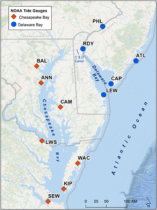
Figure 1. Map of the Delaware and Chesapeake Bays with the 12 NOAA tide gauges used in the current study: PHL, Philadelphia; RDY, Reedy Point; CAP, Cape May; ATL, Atlantic City; BAL, Baltimore; ANN, Annapolis; CAM, Cambridge; LWS, Lewisetta; KIP, Kiptopeke; SEW, Sewells Point; WAC, Wachapreague.

Water Level Data and Computation of Skew Surge

Tide gauges selected for this study were limited to NOAA operational tide gauges in and immediately around the Delaware and Chesapeake Bays. Requirements were that each gauge maintained nearly continuous record of hourly water levels for the time period 1980–2019, evenly located throughout the region, a set of harmonic constituents identified for making tidal predictions, and a vertical tidal datum conversion factor to North American Vertical Datum of 1988 (NAVD88). In all, 12 gauges were selected; 5 associated with the Delaware Bay and 7 with the Chesapeake (Figure 1; Table 1). All selected gauges are part of NOAA NWLON and PORTS networks.

TABLE 1

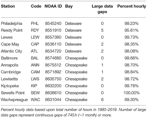
Table 1. Tide gauges used in the current study.

Hourly and High/Low water level data were obtained from the NOAA Center for Operational Oceanographic Products and Services (NOAA CO-OPS, 2020b). High/Low data represent the exact time and magnitude of each Higher-High, High, Low, and Lower-Low tidal peak. Hourly data represent the observed water level on each hour (e.g., 21:00, 22:00). The 40 years of hourly data at each gauge were manually inspected for errors and inconsistencies. A few small data clusters (of 2–16 h) within larger gaps of missing data were removed (on seven occasions across all gauges) and small data gaps of 1–2 h (<10 across all gauges) were filled using linear interpolation. Table 1 lists the number of data gaps that spanned 745 h (~1 month) or greater as well as the percentage of valid hourly data points used in the analysis. Wachapreague had the largest amount of missing data due to a 2.5-year period (200511–200804) when valid Hourly and High/Low data were unavailable.

Skew surge was computed at each tidal peak over 1980–2019 using modeled predicted time series as reference. Total count was a maximum of 28,231 tidal peaks over the study time period, less any missing data. The observed maximum TWL at each peak was extracted from the High/Low dataset; the maximum hourly value was used if High/Low data were not available. The observed and predicted peaks were aligned within ±3 h of each other, which was extended to ±6 h if no High/Low or TWL peak alignment was found, such as due to prolonged surge; this occurred for <100 peaks over the entire study time period and only for gauges in the Chesapeake Bay.

Predicted tides were generated through Harmonic Analysis (HA) based on hourly water levels. The HA incorporated 37 tidal constituents defined by NOAA for their official tide predictions in this region (NOAA CO-OPS, 2020c) and seven tidal constituents noted by Harris (1991) relevant for the US East Coast. Computations were performed in 1-year increments (3-year increments if greater than 1 month of data were missing within a year). Annual computations minimize timing errors that can lead to the leakage of tidal energy into the non-tidal residual (Merrifield et al., 2013). It also essentially removes the SLR trend and minimizes inherent constituent biases when computed over long time periods, which could result from changing physiographical environmental conditions (Ross et al., 2017) or from changing seasonal weather patterns that strongly influence the Sa (solar annual) and SSa (solar semi-annual) constituents (NOAA CO-OPS, 2007). More details on the computation of skew surge can be found in Callahan et al. (2021a).

Mean and standard deviation of skew surge, as well as maximum TWL for comparison, were computed to get a sense of the overall parent distribution. To help achieve stationarity and independence of data samples required by EVA, two further processes were performed on each gauge's time series. First, the data were linearly detrended about the 1980–2019 mean (Table 2). Second, maximum peaks of skew surge were separated temporally by 30 h to ensure at least two high tides between each extreme event. Specifically, multiple surges above each selected threshold (defined following approaches in Block Maxima/GEVr Approach and Points-Over-Threshold/GP Approach sections) within 30 h of each other were treated as from a single event and only the maximum value was chosen.

TABLE 2

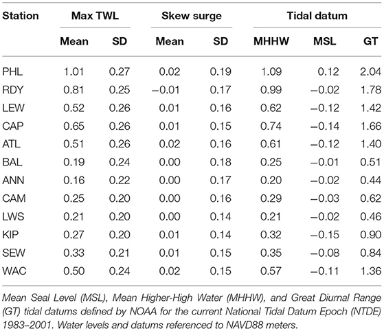
Table 2. Mean and standard deviation of maximum total water level (TWL) and skew surge for all tidal peaks observed during 1980–2019.

Block Maxima/GEVr Approach

The BM approach of modeling extreme values is to select the maximum value within equal, independent blocks of time over the study period, which are usually fit to the GEV distribution. One-year blocks are commonly chosen (as in the current study) since a common ultimate goal is to estimate water levels of multiyear-based return periods for long-term planning purposes. Using the BM approach in this traditional way results in 40 data points over the years 1980–2019. The GEV distribution actually represents the combined generalized form of the Fréchet, Weibull, and Gumbel distributions, which have cumulative distribution functions (CDF) defined by Equation 2.1.

$\begin{array}{l}F\left(x|\mu ,\sigma ,\xi \right)\hfill \\ =Pr\left(X>x\right)=\hfill \end{array}\{\begin{array}{cc}\exp \left[-{\left(1+\xi \left(\frac{x-\mu }{\sigma }\right)\right)}^{-1/\xi }\right],& \xi \ne 0,\\ \exp \left[-\exp \left(-\left(\frac{x-\mu }{{\sigma }_{\mu }}\right)\right)\right],& \xi =0,\end{array}(2.1)$

where the quantity 1+ξ(x−μ)/σ = max(1+ξ(x−μ)/σ, 0), with location parameter μ, scale parameter σ > 0, and shape parameter ξ. The shape parameter controls the shape of the tail. The second line of Equation 1 (ξ = 0) represents the Gumbel distribution and is found by taking the limit as ξ → 0. When ξ > 0 (Frechet), the tail is thicker than the Gumbel (i.e., “heavy-tailed”) with no upper bound, whereas for ξ < 0 (Weibull), the distribution has a hard upper limit at μ – σ/ξ. Coles (2001) provides a detailed description of the BM/GEV approach.

A drawback of this approach is the limited number of data points (i.e., one per year) used to fit the model. Therefore, this method was generalized to include more than one value for each independent block of time by Weissman (1978) and later justified for use in hydrological studies, including modeling sea level extremes, by Tawn (1988). This extension of the BM approach allows for the use of the r-largest order statistics per year, permitted that r < < total number of events per year. The key distinction of fitting data to the GEVr distribution, as opposed to the GEV distribution, is the choice of r. At r = 1, the GEV and GEVr are identical distributions. Since r is not a specific parameter in the GEVr probability density function, it cannot be estimated in the same way as μ, ξ, or σ.

Several orders of r were tested from 1 to 20 events per year. For each r, model parameters were estimated, and a series of hypothesis tests run. The upper limit choice of 20 was subjective but reasonable, as it would increase the number of data points significantly (20 × 40 years = 880, ~3% of all tidal peaks over 1980–2019) while keeping r < <730, the maximum number of twice-daily skew surge events per year. Ideally, r should be large enough to include enough points to improve the robustness of the model but not large enough to introduce bias from the parent distribution and contaminating the EVD model fit.

A set of rules were developed by G'Sell et al. (2016) and furthered by Bader et al. (2017) to automate the selection of an optimum value of r. These rules are based on the sequential hypothesis tests for each r using the ForwardStop score and unadjusted p value generated from parametric bootstrap and entropy difference tests. The ForwardStop score is an adjusted p-value to control for the incremental false discovery rate, similar to a weighted mean of p-values of all tests on previous r values (Bader et al., 2017). The over-riding principal here is to start with a minimum number of data points and slowly increase the sample size until the data points do not satisfactorily fit the GEVr distribution. Following guidance provided in Bader et al. (2017), the following procedure was adopted to identify the optimum r.

1. Start with r = 1 and note the ForwardStop score from the parametric bootstrap test. Incrementally increase r by 1 until the ForwardStop score fails hypothesis test at the α = 0.05 level. If a failure occurs, that r is rejected and select the r just prior to the failed test.

2. If no r values are rejected after traversing all 20, use the ForwardStop score from the entropy difference test and repeat Step 1.

3. If no r values were rejected following Step 2, then repeat Steps 1–2 using the unadjusted p-values computed for each r instead of the ForwardStop score.

4. If no r values were rejected following Step 3, increase α to 0.10 and repeat Steps 1-3.

Using these guidelines, an optimum r was selected for each gauge. The Goodness-of-Fit (GoF) was then tested between the Gumbel distribution (ξ = 0) fit and the Fréchet/Weibull distribution (ξ ≠ 0) fit using the negative log-likelihood ratio test (ratio must be greater than 0.95) and Akaike Information Criterion (AIC) test (the difference in AIC score between sequential tests must be > 2, described in Burnham and Anderson, 2004). Maximum likelihood estimation (MLE) was used for all GEVr model fits. Temporal declustering of skew surge peaks was performed on an annual basis in order for each of the r-largest orders per year to be an independent event.

Points-Over-Threshold/GP Approach

In contrast to the BM approach, the POT approach is a more natural way of statistically modeling the upper tail of a parent distribution. The entire study period is treated as a single block and the EVD includes only observations over a certain threshold value (i.e., exceedances) regardless of time the event occurred. The threshold is derived from a suitably high quantile level (e.g., 97% quantile is commonly used). Exceedances are then fit to the Generalized Pareto (GP) distribution. Like the GEV, the GP distribution represents a family of three distributions, differentiated by the model shape parameter, the CDFs of which are in Equation 2.2.

$\begin{array}{l}F\left(x|\mu ,{\sigma }_{\mu },\zeta \right)\hfill \\ =Pr(X<x|X>\mu )=\hfill \end{array}\{\begin{array}{cc}1-{\left[1+\xi \left(\frac{x-\mu }{{\sigma }_{\mu }}\right)\right]}^{-1/\xi },& \xi \ne 0,\\ 1-exp\left[-\left(\frac{x-\mu }{{\sigma }_{\mu }}\right)\right],& \xi =0,\end{array}(2.2)$

where the quantity inside the brackets [y] = max([y], 0), suitably high threshold μ, threshold-dependent scale parameter σ_μ > 0, and shape parameter ξ. The condition is that all values of x must be larger or equal to the threshold μ. Behavior of the parameters is similar to that in the GEV. The shape parameter controls the shape of the tail. The second line of Equation 2.2 is found by taking the limit as ξ → 0, resulting in the Exponential distribution. A heavy tail occurs when ξ > 0 (Pareto distribution) with no upper bound, whereas a thinner tail and a fixed upper bound occurs when ξ < 0 (Beta distribution). Coles (2001) provides a detailed description of the POT/GP approach.

Threshold quantiles were tested from 90–99.5% exceedance probabilities in increments of 0.5% (from 1 to 20 thresholds), resulting in the maximum number of possible skew surge peaks used to model GP to be ~2,920 (90%) to 146 (99.5%). A threshold should be chosen to include enough upper tail exceedances that will improve the robustness of the model but not too many exceedances such that the lower values introduce bias from the parent distribution. Scarrott and MacDonald (2012) reviewed various methods on selecting the optimum threshold, including numerical tests and graphical diagnostics, such as Quantile-Quantile and Mean Residual Life plots. Many of these selection methods are subjective, time-consuming when investigating many sites, and often result in multiple acceptable answers. Diagnostic plots were used in the current study (Supplementary Figures 1–24), however, to better compare results with BM/GEVr approach, a similar standardized methodology was employed for selecting an optimum threshold.

The rules developed by G'Sell et al. (2016) and Bader et al. (2017) were applied to automate the selection of the optimum threshold of the POT/GP approach in Bader et al. (2018). Unadjusted p-values from Anderson-Darling test were chosen in Bader et al. (2018) for threshold sequential hypothesis testing after a comparison among several other GoF tests. Although, Bader et al. (2018) recommends using ForwardStop score, based on skew surge data in the current study, ForwardStop rejects very few thresholds and the unadjusted p-values performed well in Bader et al. (2018) tests. Using the same over-riding principal here as with the BM/GEVr approach, start with the least number of data points and slowly increase the sample size until the data points do not satisfactorily fit the GP model. This is essentially working backwards, from the highest to lowest threshold, noted as the RawDown approach in Bader et al. (2018). A RawUp approach, working upwards from the minimum threshold (i.e., most data points) until a hypothesis test was accepted, was also described in Bader et al. (2018) but carries a higher chance for contaminating the EVD than the RawDown approach. Ultimately, the following rules were adopted to identify the optimum threshold.

1. Start with highest threshold percentage (99.5%) and note the unadjusted p-value from the Anderson-Darling test. Incrementally decrease the threshold percentage by 0.5% until the GP model fit fails hypothesis test at α = 0.05 level. If a failure occurs, that threshold is rejected and select the threshold just prior to the failed test.

2. If the highest threshold (99.5%) is rejected on the first test but the second (99.0%) is not rejected, then skip the highest threshold and continue working downward until next rejection occurs. This allows for the opportunity to include more exceedances in the model and assumes the rejection occurred by chance.

3. If no thresholds were rejected following Step 2, increase α to 0.10 and repeat Steps 1–2.

Using these guidelines, an optimum threshold was selected for each gauge. Temporal declustering was performed separately for each threshold on all exceedances over the entire study period at once. Declustering therefore significantly reduced the actual number of skew surge events used in fitting the GP model by ~30–70%. As with the GEVr model, MLE was used for all GP model fits.

Skew Surge Return Levels

Lastly, return level (RL) skew surges were estimated for 1.1, 3, 5, 10, 25, 50, and 100-year return periods for each EVA modeling approach. A RL represents a threshold that the probability of exceedance in any 1 year is the inverse of the return period. For example, 100-year RL has a 1.0% (0.01) probability of being exceeded in any 1 year. Since the 1-year RL is undefined within the BM/GEVr approach, 1.1-year was used instead for comparison.

Although probability quantiles can be easily extracted from the GP theoretical distribution using the fitted parameters, they cannot be viewed as annual probabilities of return levels, such as can be done using the BM/GEVr approach. Therefore, an estimate of the probability of a skew surge exceeding a selected threshold in a year on average must be included in RL calculations using the POT/GP approach. This is found by dividing the total number of declustered skew surge events above the selected threshold by the total number of years (40).

A qualitative review was performed on the estimated model parameters and return levels, with their 95% standard errors (SE) modeled using the selected optimum r (BM/GEVr) and threshold (POT/GP). Differences between the EVA modeling approaches and spatial variations were noted.

The harmonic analysis and tidal data processing work was done using the U-Tide package (Codiga, 2011) and standard modules in the Matlab programming environment. Temporal declustering was performed using the POT package (Ribatet and Dutang, 2019) and the EVA model fitting and RL extraction were performed using the eva package (Bader and Yan, 2020), both of the R statistical computing software environment.

Results

Skew Surge

Mean skew surges are consistent and very close to zero across all tide gauges whereas TWL shows much larger geographic variation (Table 2). Although differences are minor, largest skew surges (0.2 m) are at PHL and the open ocean gauges at ATL and WAC. TWL is consistently higher in the Delaware Bay than the Chesapeake Bay. Within each bay, the Delaware Bay upper regions have higher max TWL than the lower regions, whereas this pattern is reversed in the Chesapeake Bay. Spatial pattern of max TWL aligns with the Mean Higher-High Water (MHHW) and Great Diurnal Range (GT) tidal datums (Figure 3), which do not align with the spatial pattern of skew surge. Standard deviations of skew surge show slightly more geographic variation (ranging 0.14–0.19 m) with a similar spatial pattern to the max TWL and Mean Sea Level (MSL) tidal datum. Largest deviations are in the upper bays and lowest in the central Chesapeake Bay.

None of the gauges showed statistically significant trends in skew surge except for PHL, which showed a slight negative trend of ~ −0.3 mm/year, nevertheless, all gauge time series were detrended. Note that for comparison, all gauges showed statistically significant increasing trends in max TWL consistent with local SLR rates (further analysis was not performed on max TWL within this study.)

As an example of the parent vs. upper tail distributions, Figure 2 (left panel) shows the histogram of all detrended skew surges for the LEW tide gauge over the entire study time period with a zoomed-in view of the upper tail (right panel). The Normal distribution fit the parent distribution at p < 0.01, yet significantly underestimates the empirical data in much of the upper tail, emphasizing the importance of modeling extremes of skew surge separately from the parent distribution.

FIGURE 2

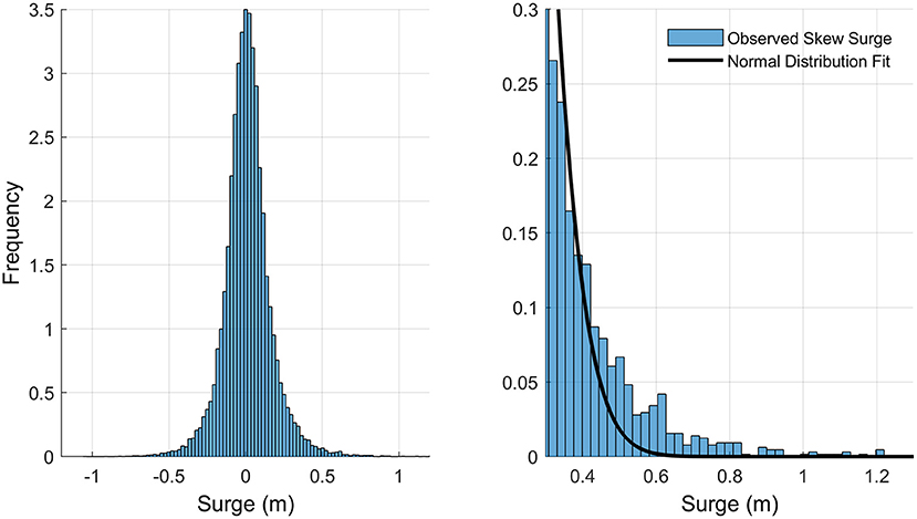
Figure 2. Example demonstrating the “fat tail” nature of skew surge distribution for the NOAA tide gauge at Lewes, DE. Histogram includes all detrended skew surges over 1980–2019 (left panel). Upper tail of the same data with Normal distribution model fitted to all data points (right panel). Note the upper tail of the theoretical parent distribution under-represents empirical skew surge.

Model Parameter Selection

Figure 3 shows an example of the GEVr sequential hypothesis testing for the LEW gauge. No rejections occurred (below α = 0.05) using ForwardStop score from either the parametric bootstrap or entropy difference procedures. Starting from r = 1 and sequentially comparing the unadjusted p-values, the first rejection occurs at r = 15, resulting in the optimum r = 14. Testing for the optimum threshold in the POT/GP approach worked in the same way, albeit starting on the right side of the unadjusted p-values plot and working downward until a rejection occurs following guidance in Points-Over-Threshold/GP Approach Section.

FIGURE 3

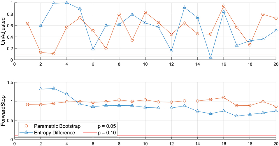
Figure 3. Example demonstrating GEVr Unadjusted p-values (top panel) and ForwardStop (bottom panel) results based on the Parametric Bootstrap and Entropy Difference tests for r = 1–20, as defined in Bader et al. (2017). Following the guidelines outlined for the current study, optimum r = 14. Skew surge data for the NOAA Lewes tide gauge over 1980–2019.

Table 3 and Figure 4 show resultant model parameters estimated after selecting the optimum r in the BM/GEVr approach at each gauge. The number of skew surge events per year that were fit to the GEVr distribution, ranges from N = 120 (r = 3 at CAP, ANN, SEW) to N = 560 (r = 14 at LEW). Both the location and scale parameters have small, consistent SE relative to their magnitude across all sites. The shape parameter is the most uncertain of all the parameters, although SE is relatively consistent across all sites. Uncertainty is inversely related to the total number of skew surge events ultimately used in the EVA after declustering; the lower the number of events, the smaller the SE. Shape parameter is positive at all sites except at WAC where it is slightly negative. Based on the negative log-likelihood ratio and AIC difference tests, none of sites favor the use of the GEVr Gumbel (ξ = 0) distribution over the GEVr Fréchet/Weibull (ξ ≠ 0) distribution.

TABLE 3

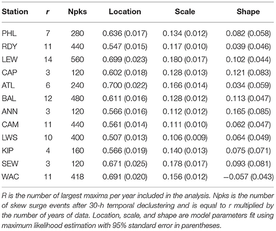
Table 3. Results from GEVr distribution model fit of extreme skew surges for tide gauges in the Mid-Atlantic region.

FIGURE 4

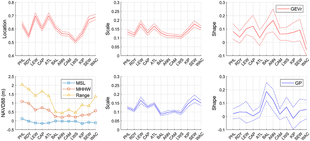
Figure 4. Model fit parameters of extreme skew surges to the GEVr (red, top row) and GP (blue, bottom row) distributions. Location is a model parameter only for GEVr distribution. Dotted lines represent the 90% confidence interval. Mean Sea Level (MSL), Mean Higher-High Water (MHHW), and Great Diurnal Range (GT) tidal datums defined by NOAA for the current National Tidal Datum Epoch 1983–2001 referenced to NAVD88 meters.

Similarly, Table 4 and Figure 3 summarize the results after selecting the optimum threshold using the POT/GP approach at each gauge. Threshold percentages range from 94.5% (ATL, N = 732) to 99.0% (LEW, ANN, KIP, and SEW, N = 160, 194, 139, and 142, respectively.) Gauges that have the same optimum threshold still result in different total number of skew surge events due to temporal declustering. Scale parameter SE is low while the shape parameter SE is relatively high across all sites. Shape parameter is positive at all sites except at KIP where it is slightly negative. Spatial patterns and relative uncertainties of both the scale and shape parameter estimates are generally similar between the two approaches.

TABLE 4

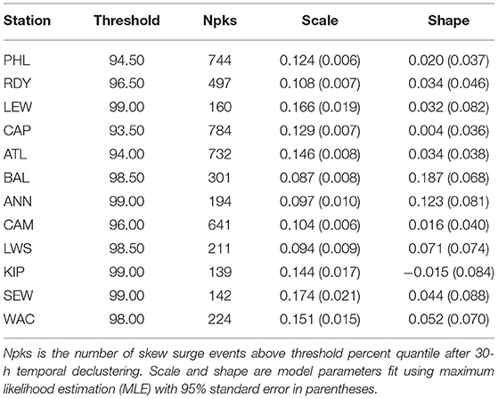
Table 4. Results from GP distribution model fit of extreme skew surges for tide gauges in the Mid-Atlantic region.

Supplementary Figures 1–12 (BM/GEVr) and 13–24 (POT/GP) show diagnostic plots of the model fit using the optimally selected r and threshold values at each tide gauge. Included are probability-probability (PP) and quantile-quantile (QQ) plots of the modeled vs. empirical data, and histograms overlaid with model fit PDF curve. The PP plots and histograms show good agreement between the model and observations. For most gauges, the QQ plots show a few outliers with the observed skew surge levels higher than modeled quantile estimates. The LEW gauge did not show this behavior but rather at the largest values, the modeled quantiles were larger than the observed data.

Skew Surge Return Levels

Skew surge return levels for 1.1, 3, 5, 10, 25, 50, and 100-year return periods with 90% confidence intervals (i.e., uncertainty) are shown in Table 5 for BM/GEVr and Table 6 for POT/GP. For the sake of brevity and ease of comparison, only the mean values are plotted in Figure 5. Note the more traditional continuous RL curves with confidence intervals are included in Supplementary Figures 25–26, and additionally plotted with empirical data in panel 4 of Supplementary Figures 1–24. RLs increase in a consistent manner with longer return periods at all sites under both modeling approaches. For BM/GEVr, 100-year RLs range from 1.07 m (LWS) to 1.79 m (LEW) with generally largest values starting in the lower bay regions, decreasing to a minimum in the central regions, then increasing toward the upper regions. This pattern is similar across all RLs. LEW and SEW have the largest RLs for most return periods, except for the 1.1-year return period, where the maximum RL is at ATL (although several other sites are very close). Longer return periods demonstrate more spatial variation in RLs. Using POT/GP, 100-year RLs range from 1.08 m (LWS) to 1.56 m (LEW), with approximately the same spatial pattern as with BM/GEVr.

TABLE 5

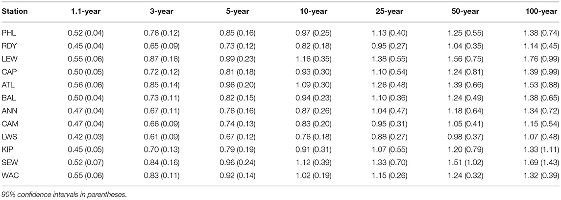
Table 5. Estimated skew surge return levels for 1.1, 3, 5, 10, 25, 50, and 100-year return periods modeled using the BM/GEVr approach for tide gauges in the Mid-Atlantic region.

TABLE 6

Table 6. Estimated skew surge return levels for 1.1, 3, 5, 10, 25, 50, and 100-year return periods modeled using the POT/GP approach for tide gauges in the Mid-Atlantic region.

FIGURE 5

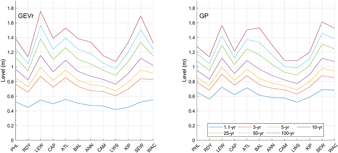
Figure 5. Estimated skew surge return levels for periods of 1.1, 3, 5, 10, 25, 50, and 100 years using the BM/GEVr (left panel) and POT/GP (right panel) approaches for tide gauges in the Mid-Atlantic region, 1980–2019.

There are few differences in RLs between approaches (Table 7; Figure 6). The most noticeable is that the 1.1-year RLs using BM/GEVr (0.45–0.56 m) are significantly lower than using POT/GP (0.52–0.72 m) at all sites. At the other extreme, BM/GEVr 100-year RLs are generally higher, mostly in the upper bay regions, with LEW (0.19 m) and CAP (0.17 m) showing the largest positive differences between methods. BAL (−0.15 m) and WAC (−0.20 m) are exceptions, with higher 100-year RLs using POT/GP. Most return periods between 3-year and 50-year show small differences in RLs across most gauges.

TABLE 7

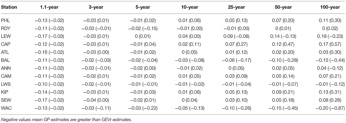
Table 7. Difference in estimated skew surges and 90% confidence intervals (in parentheses) for 1.1, 3, 5, 10, 25, 50, and 100-year return periods modeled from GEVr and GP distribution for tide gauges in the Mid-Atlantic region.

FIGURE 6

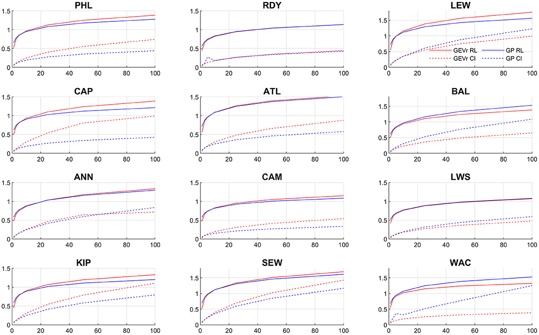
Figure 6. Estimated return levels (solid line) and 90% confidence intervals (dotted line) using the BM/GEVr (red line) and POT/GP (blue line) approaches.

Uncertainty also increases with longer return periods under both approaches, as expected. At 1.1-year return period the uncertainties are < 0.10 m, and range 0.18–0.39 m at 10-year, and 0.30–1.43 m at 100-year. Sites in the Chesapeake Bay, under both approaches, exhibit spatial variation in uncertainty similar to that of the mean RL estimates, with the largest uncertainties in the lower bay regions, smallest in the central regions, and increasing in the upper regions. WAC is an exception to this with small uncertainty under BM/GEVr. Sites in the Delaware Bay also show this same pattern in uncertainty with BM/GEVr but not POT/GP, under which CAP and ATL (sites in the lower bay region) show small uncertainties.

Generally, uncertainties under both approaches are very similar to each other at shorter return periods. At longer return periods in the Delaware Bay, uncertainties are smaller using POT/GP for most sites. At longer return periods in the Chesapeake Bay, generalization is more difficult; BAL (−0.44 m at 100-year) and WAC (−0.87 m at 100-year) have significantly smaller uncertainties using BM/GEVr while many other sites have smaller uncertainties using POT/GP.

Discussion

The focus areas of the current study is to investigate the magnitude and geographic variation within the Delaware and Chesapeake Bays of estimated return levels of skew surge for ~1-year to 100-year return periods and to compare the two most common traditional EVA approaches. Although skew surge is arguably one of the best and simplest measures of the meteorological drivers of coastal flooding, as it is the portion of flood depth above the high tide level, its wider use in literature has only recently gained attention. This work was done strictly through empirical data (rather than using simulated events or scenario-based projections) over the past 40 years and statistically analyzed through stationary EVA on detrended skew surges. Observational data showed minimal trends over this time period, hence results from this study should not be appreciably different than non-stationary EVA that allows for temporally varying or multivariable dependent location and scale parameters. To test the robustness of the methods, the POT/GP approach presented here was applied to max TWL and resulting return levels compared against those found in U. S. Army Corps of Engineers (2014), who performed a similar EVA using longer time periods. Seven tide gauges were analyzed in both studies: LEW, CAP, ATL, BAL, ANN, CAM, and SEW. Although they used different thresholds, detrending methods, and reference periods, the general spatial and temporal trends were consistent between the two studies, including the intervals between the 50-year and 100-year RLs. Largest differences were found for longer return periods at BAL and ANN, sites that have experienced extreme coastal flooding outliers (Callahan et al., 2021b).

Due to the approximate independence of skew surge to SLR and tidal phase (i.e., likely minor influences of tide-surge interactions at our sites), extreme return levels can reasonably be linearly added to future SLR scenarios as a first approximation for planning (Delaware Flood Avoidance Workgroup (DE FAW), 2016; Federal Emergency Management Agency (FEMA), 2016). For example, if a structure is designed to withstand the 50-year flood event, the 50-year return levels can be added to the expected high tide (either the MHWW or Highest Astronomical Tide datum) under an appropriate SLR planning scenario. It should be noted that skew surge computed in this study includes contributions from other aspects associated with extreme flooding events, such as nearby river discharge and wave setup, which ultimately likely benefits many long-term planning activities. As well, trends in skew surge were minor and mean values were within a few centimeters of zero over 1980–2019 (Table 2), however, an adjustment to skew surge RLs due to detrending could be performed. Care is warranted when making linear adjustments too far into the future due to the expected exponential increase in SLR and uncertainty in future extreme storm conditions along the Mid-Atlantic (Callahan et al., 2017, 2021b).

Largest return levels across most return periods occur within the bay boundaries in the lower regions, and not in the upper regions of the bays and ocean coast sites that typically show higher surges and TWLs. Specially, LEW and SEW gauges, both located on the southwest side of the mouth of each bay, consistently show the largest RLs throughout the region. One explanation is that many large coastal flood events are associated with ETCs, often as traditional nor'easters. For these storms, the low-pressure center off the coast brings strong northeast winds, which drives enhanced surges into the bays through Ekman transport as well as direct winds piling up water on the southwest sides of the lower bays. This would be most effective in the lower Delaware Bay, where the width of the Bay reaches 45 km. The upper Delaware Bay, although it experiences large tidal ranges and increased surges (due to conical shape of coastline and from the increased volume of water entering the bay from southeasterly to easterly winds), may not experience the worst impacts from the most extreme storm events and may actually see decreases in surges from northerly winds that also occur during nor'easters. The upper Chesapeake Bay does not exhibit the same high TWL, MHHW, or surges as in the upper Delaware Bay (primarily due to the overall size, shape, and depth of the Chesapeake Bay), however, extreme skew surge RLs in both upper regions are comparable to each other. This supports results in Callahan et al. (2021a), which found the upper bays were highly correlated with each other from TC-caused skew surges, more so than with their respective lower bay regions. TCs can account for close to 40–60% of the largest (top 10) coastal flooding events in the Mid-Atlantic, with smaller relative percentages over larger number of events (Booth et al., 2016; Callahan et al., 2021b). In particular for the upper Chesapeake Bay, Hurricane Isabel in 2003 caused extreme coastal flooding compared to other events, directly influencing higher return period RLs and their uncertainties.

RLs tend to be at a minimum within each bay closer to the central regions, CAM and LWS in the Chesapeake and RDY in the Delaware Bays. These areas have the lowest mean skew surges throughout the region and typically do not experience the worst wind-driven impacts from coastal storms. Likewise, these areas also exhibit the smallest uncertainties throughout the region across many return periods.

A secondary focus of this study is to provide insight into the two most common approaches of stationary EVA applied to Mid-Atlantic skew surge. To that end, the GEVr distribution was combined with the BM approach to address the small sample size of the traditional annual max BM/GEV approach, and a standardized method for selecting optimum r and threshold was incorporated. The use of GEVr increases the robustness of the model fit and puts the number of data points more comparable to the POT/GP approach, however, there are some disadvantages of using a BM approach. Large surge events could be missed, for example, if an individual year has more major coastal flood events than the selected optimum r (i.e., false positives). At the other end, non-extreme surge events could be included, for example, if an individual year has less major coastal flood events than the selected optimum r, introducing bias from the parent distribution (i.e., false negatives). Use of the POT/GP approach circumvents these issues as it is irrespective of time, solely focused on the upper tail of the parent distribution. A potential trade-off is if the majority of extreme events occur toward either end of the study time period, direct interpretation of annual return levels from the mean number of events per year is more difficult. From review of the data used in the current study, clustering of major skew surge events occurring on either end of the time period was not present.

The choice of optimum r or threshold is a tricky problem to address. It is usually a subjective process, including graphical and numerical diagnostic information, and choosing among multiple appropriate candidates. The current study incorporates a standardized methodology of sequential hypothesis texting that can be applied to all sites simultaneously while allowing for variable r/threshold selection per site. Although stopping rules and goodness of for tests are still subjective within this methodology, they are data-driven, based on statistical results from Bader et al. (2017, 2018). Choice of stopping rules influences the number of data points (r-largest orders or threshold exceedances), and hence, directly influence the uncertainty in model parameters. Uncertainty in RLs do not consistently show strong dependence on the number of peaks included in the model fit. This potential relationship of RL uncertainty and optimum r/threshold should be explored further in future work.

Changes in storm frequency and intensity (“storminess”), either observed or projected due to climate change, were not addressed in this study. As stated above, skew surge is closely related to the meteorological characteristics driving the flooding and relatively independent of SLR or tides. Trends in skew surge are therefore influenced by oscillations and trends in oceanic-atmospheric circulation patterns that support enhanced cyclogenesis or steer storms along the coast. Common teleconnections associated with the frequency or magnitude of surges in the Mid-Atlantic region include the North Atlantic Oscillation, Pacific-North American oscillation, El Nino/Southern Oscillation, and Atlantic Meridional Overturning Circulation, several of which have been included as covariates in non-stationary EVA or joint-probability models of surges in recent years (Ezer et al., 2013; Sweet et al., 2014; Hamlington et al., 2015; Wahl and Chambers, 2015; Kopp et al., 2019; Little et al., 2019; Rashid Md et al., 2019). The 40-year time period of the current study is long enough to capture several oscillations of many of these teleconnections, essentially averaging out their influence. Extreme RLs then can be viewed as based on relative average synoptic conditions, however, the probability of occurrence of an extreme surge event in any single year is dependent upon the presence and strength of teleconnection patterns, and assessment should be performed as near to the year in question as possible.

Other aspects of this study could have influenced extreme surge estimates. Most notably is the length of the data record, as is usually the case in EVA. Although there exists general agreement with results in U. S. Army Corps of Engineers (2014), 40 years of data to estimate 100-year RL is not ideal. Comparing EVA results on skew surge using the methods presented in the current study on a subset of gauges with much longer records, perhaps one gauge per sub-bay region, could offer insight into the robustness of the current study statistical results. Additionally, the set of 44 constituents used in the HA computation of the predicted tide may not capture all the tidal oscillations present at every site, thereby impacting the magnitude of skew surge (albeit these changes likely would be minimal). The choice of 30 hours was subjective and may not be optimum at all sites to separate individual skew surge events, although it is rare for a single storm event to reach extreme surge levels multiple times separated by two or more high tides.

Conclusion

Understanding extreme events is important because of their potential for disproportionate damage and threat to public health, which will aid in mid- to long-term planning of many coastal communities and critical ecosystems along their shores. Across most of the return periods, the largest return levels occur at LEW and SEW, which are within the bay boundaries in the southwest side of the lower regions of their respective bay. Likewise, minimum return levels occur near the central regions of each bay, at RDY and LWS. This may seem counterintuitive for the Delaware Bay where the upper bay (PHL) experiences high water levels and tidal ranges but is consistent with wind and ocean current patterns for offshore storms in this region.

Determination of which approach is “best” for modeling extreme skew surge events in the Mid-Atlantic is not a goal of the current study. Nevertheless, differences between the approaches are highlighted and some general recommendations can be made. Overall, both approaches provide similar results. Confidence in model parameters is good and consistent across all sites between both approaches, with narrow confidence intervals for the location and scale parameters. Confidence is less for shape parameter but is generally the same for both approaches. Not many differences in magnitude of RLs exist, especially for 3-year to 100-year return periods, which helps justify comparisons of extreme levels of surge among previous EVA studies in this region (at least for skew surge).

For the 1.1-year return period, the POT/GP approach provides more consistent values in respect to other return periods across both bays. This is likely due to the effects of estimating RLs from the GEVr distribution close to 1-year. For the Delaware Bay at longer return periods, the POT/GP also seems to perform well (lower uncertainty) at most sites and therefore could be used at all return periods up to 100 years. This finding is supported by U. S. Army Corps of Engineers (2014) statements that traditional BM/GEV approach tends to overestimate and have larger uncertainties when compared to POT/GP. Recommendations are more mixed for the Chesapeake Bay for return periods at 3-year and above. Results at ANN and LWS are nearly identical for both approaches. For KIP and SEW, sites in the lower Chesapeake Bay, lower uncertainties and slightly lower RLs tend toward the POT/GP approach. Conversely, BAL (upper region) and WAC (ocean coast) tend toward the use of the BM/GEVr approach.

Data Availability Statement

The datasets presented in this study can be found in online repositories. The names of the repository/repositories and accession number(s) can be found below: the dataset of extreme skew surge return levels, estimated using both BM/GEVr and POT/GP approaches, at each tide gauge analyzed for this study can be found at the figshare repository, https://figshare.com/account/home#/projects/101024.

Author Contributions

JC and DL conceived the idea of investigating extreme coastal flood levels in the U.S. Mid-Atlantic Delaware and Chesapeake Bays. JC designed the analysis framework, obtained all the necessary data, performed the statistical analysis, and wrote the manuscript. DL helped with results interpretation and manuscript revisions. All authors contributed to the article and approved the submitted version.

Benefit of Research to Scientific Community

Extreme storm surges can overwhelm many coastal flooding protection measures in place and cause severe damages to private communities, public infrastructure, and natural ecosystems, particularly in the Mid-Atlantic region. However, by definition, extreme events are rare and difficult to model due to small sample sizes. Results from this study provide estimates of extreme skew surge, a less often studied but robust measure of the meteorological component of coastal flood levels, for return periods of 1.1 to 100 years. This study also aims to increase understanding and reliability of projections of extreme water levels using methods commonly found in the literature and ultimately help in long-term planning of mitigation and implementation of adaptation measures.

Conflict of Interest

The authors declare that the research was conducted in the absence of any commercial or financial relationships that could be construed as a potential conflict of interest.

Publisher's Note

All claims expressed in this article are solely those of the authors and do not necessarily represent those of their affiliated organizations, or those of the publisher, the editors and the reviewers. Any product that may be evaluated in this article, or claim that may be made by its manufacturer, is not guaranteed or endorsed by the publisher.

Acknowledgments

The authors would like to thank the National Oceanic and Atmospheric Administration for providing a large database of water level data for public use. The authors would also like to thank Dr. Daniel L. Codiga, Graduate School of Oceanography, University of Rhode Island, and Dr. Richard Pawlowicz, Department of Earth, Ocean and Atmospheric Sciences, University of British Columbia, for their help in understanding the operation of U-Tide and performing harmonic analysis.

Supplementary Material

The Supplementary Material for this article can be found online at: https://www.frontiersin.org/articles/10.3389/fclim.2021.684834/full#supplementary-material

NOAA Tide Gauge Locations:

PHL, Philadelphia; RDY, Reedy Point; LEW, Lewes; CAP, Cape May; ATL, Atlantic City; BAL, Baltimore; ANN, Annapolis; CAM, Cambridge; LWS, Lewisetta; KIP, Kiptopeke; SEW, Sewells Point; WAC, Wachapreague.

Abbreviations:

BM, Block Maxima; ETC/TC, extratropical cyclone/tropical cyclone; EVA/EVD, extreme value analysis/extreme value distribution; GEV, generalized extreme value distribution; GEVr, generalized extreme value r-largest order distribution; GoF, goodness-of-fit test; GP, Generalized Pareto distribution; HA, harmonic analysis; MLE, maximum likelihood estimation; MHHW, Mean Higher-High Water tidal datum; MSL, Mean Sea Level tidal datum; NAVD88, North American Vertical Datum of 1988; NTDE, National Tidal Datum Epoch; NTR, non-tidal residual; NWLON, NOAA NOS National Water Level Observation Network; PORTS, NOAA National Ocean Service Physical Oceanographic Real-Time System; POT, points over threshold; RL, return level; SLR, sea-level rise; SST, sea surface temperature; SE, standard error; TWL, total water level.

References

Bader, B., and Yan, J. (2020). eva: Extreme Value Analysis with Goodness-of-Fit Testing. R package version 0.1.2

Bader, B., Yan, J., and Zhang, X. (2017). Automated selection of r for the r largest order statistics approach with adjustment for sequential testing. Stat. Comput. 27, 1435–1451. doi: 10.1007/s11222-016-9697-3

CrossRef Full Text | Google Scholar

Bader, B., Yan, J., and Zhang, X. (2018). Automated threshold selection for extreme value analysis via ordered goodness-of-fit tests with adjustments for false discovery rate. Ann. Appl. Stat. 12, 310–329. doi: 10.1214/17-AOAS1092

CrossRef Full Text | Google Scholar

Batstone, C., Lawless, M., Tawn, J., Horsburgh, K., Blackman, D., McMillan, A. D., et al. (2013). A UK best-practice approach for extreme sea-level analysis along complex topographic coastlines. Ocean Eng. 71, 28–39. doi: 10.1016/j.oceaneng.2013.02.003

CrossRef Full Text | Google Scholar

Bernier, N. B., and Thompson, K. R. (2006). Predicting the frequency of storm surges and extreme sea levels in the northwest Atlantic. J. Geophys. Res. Oceans 111:10. doi: 10.1029/2005JC003168

CrossRef Full Text | Google Scholar

Blake, E. S., and Gibney, E. J. (2011). The Deadliest, Costliest, and Most Intense United States Tropical Cyclones From 1851 to 2010 (and Other Frequently Requested Hurricane Facts). NOAA Technical Memorandum NWS NHC-6

Google Scholar

Boesch, D. F., Boicourt, W. C., Cullather, R. I., Ezer, T., Galloway, G. E. Jr., et al. (2018). Sea-level Rise: Projections for Maryland 2018. Cambridge, MD: University of Maryland Center for Environmental Science

Boon, J. D., Mitchell, M., Loftis, J. D., and Malmquist, D. L. (2018). Anthropogenic Sea Level Change: A History of Recent Trends Observed in the U.S. East, Gulf and West Coast Regions. Special Report No. 467 in Applied Marine Science and Ocean Engineering. Gloucester Point, VA: Virginia Institute of Marine Science.

Google Scholar

Booth, J. F., Rider, H. E., and Kushnir, Y. (2016). Comparing hurricane and extratropical storm surge for the Mid-Atlantic and Northeast Coast of the United States for 1979–2013. Environ. Res. Lett. 11:094004. doi: 10.1088/1748-9326/11/9/094004

CrossRef Full Text | Google Scholar

Burnham, K. P., and Anderson, D. R. (2004). Multimodel inference: understanding AIC and BIC in model selection. Sociol. Methods Res. 33, 261–304. doi: 10.1177/0049124104268644

CrossRef Full Text | Google Scholar

Calafat, F. M., and Marcos, M. (2020). Probabilistic reanalysis of storm surge extremes in Europe. Proc. Natl. Acad. Sci. USA. 117, 1877–1883. doi: 10.1073/pnas.1913049117

PubMed Abstract | CrossRef Full Text | Google Scholar

Callahan, J. A., Horton, B. P., Nikitina, D. L., Sommerfield, C. K., McKenna, T. E., and Swallow, D. (2017). Recommendation of Sea-Level Rise Planning Scenarios for Delaware: Technical Report. Delaware Department of Natural Resources and Environmental Control (DNREC) Delaware Coastal Programs.

Callahan, J. A., Leathers, D. J., and Callahan, C. L. (2021a). Skew surge and storm tides of tropical storms in the Delaware and Chesapeake Bays for 1980–2019. Front. Clim. 86. doi: 10.1002/essoar.10506586.1

CrossRef Full Text | Google Scholar

Callahan, J. A., Leathers, D. J., and Callahan, C. L. (2021b). Comparison of Extreme Coastal Flooding Events Between Tropical and Mid-Latitude Weather Systems in the Delaware and Chesapeake Bays for 1980–2019. EarthArXiv [Preprint]. Available online at: https://www.essoar.org/doi/abs/10.1002/essoar.10506864.1 (accessed April 26, 2021).

Google Scholar

Chesapeake Bay Program (2020). State of the Chesapeake. Available online at: https://www.chesapeakebay.net/state (accessed August 18, 2020).

Google Scholar

Chippy, M. R., and Jawahar, S. S. (2018). Storm surge and its effect—a review on disaster management in coastal areas. Civil Eng. Res. J. 4:555649. doi: 10.19080/CERJ.2018.04.555649

CrossRef Full Text

Codiga, D. L. (2011). Unified Tidal Analysis and Prediction Using the UTide Matlab Functions. GSO Technical Report 2011-01. Graduate School of Oceanography, University of Rhode Island

Google Scholar

Coles, S. (2001). An Introduction to Statistical Modeling of Extreme Values. London: Springer.

Google Scholar

Colle, B. A., Booth, J. F., and Chang, E. K. M. (2015). A review of historical and future changes of extratropical cyclones and associated impacts along the US East Coast. Curr. Clim. Change Rep. 1, 125–143. doi: 10.1007/s40641-015-0013-7

PubMed Abstract | CrossRef Full Text | Google Scholar

Dahl, K. A., Fitzpatrick, M. F., and Spanger-Siegfried, E. (2017). Sea level rise drives increased tidal flooding frequency at tide gauges along the U.S. East and Gulf Coasts: projections for 2030 and 2045. PLoS ONE 12:2. doi: 10.1371/journal.pone.0170949

PubMed Abstract | CrossRef Full Text | Google Scholar

Delaware Emergency Management Agency (DEMA) (2018). State of Delaware All-Hazard Mitigation Plan. DEMA.

Delaware Flood Avoidance Workgroup (DE FAW) (2016). Avoiding and Minimizing Risk of Flood Damage to State Assets: A Guide for Delaware State Agencies. Delaware Flood Avoidance Workgroup

DNREC, (2012). Preparing for Tomorrow's High Tide: Sea Level Rise Vulnerability Assessment for the State of Delaware, pp. 210. Available online at: https://documents.dnrec.delaware.gov/coastal/Documents/SeaLevelRise/AssesmentForWeb.pdf

Dupigny-Giroux, L. A., Mecray, E. L., Lemcke-Stampone, M. D., Hodgkins, G. A., Lentz, E. E., Mills, K. E., et al. (2018). “Northeast,” in Impacts, Risks, and Adaptation in the United States: Fourth National Climate Assessment, Volume II, eds D. R. Reidmiller, C. W. Avery, D. R. Easterling, K. E. Kunkel, K. L. M. Lewis, T. K. Maycock et al. (Washington, DC: U.S. Global Change Research Program), 69–742. doi: 10.7930/NCA4.2018.CH18

CrossRef Full Text | Google Scholar

Ellis, J. T., and Sherman, D. J. (2015). “Perspectives on coastal and marine hazards and disasters,” in Coastal Marine Hazards, Risks, and Disasters, eds J. F. Shroder, J. T. Ellis, and D. J. Sherman (Amsterdam: Elseiver).

Google Scholar

Ezer, T., Atkinson, L. P., Corlett, W. B., and Blanco, J. L. (2013). Gulf Stream's induced sea level rise and variability along the U.S. mid-Atlantic coast. J. Geophys. Res. Oceans 118, 685–697. doi: 10.1002/jgrc.20091

CrossRef Full Text | Google Scholar

Federal Emergency Management Agency (FEMA) (2016). Guidance for Flood Risk Analysis and Mapping Coastal Flood Frequency and Extreme Value Analysis. FEMA.

Garner, J., Mann, M. E., Emanuel, K. A., Kopp, R. E., Lin, N., Alley, R. B., et al. (2017). Impact of climate change on New York City's coastal flood hazard: Increasing flood heights from the preindustrial to 2300 CE. Proc. Natl. Acad. Sci. USA. 114, 11861–11866. doi: 10.1073/pnas.1703568114

PubMed Abstract | CrossRef Full Text | Google Scholar

Grinsted, A., and Christensen, J. H. (2021). The transient sensitivity of sea level rise. Ocean Sci. 17, 181–186. doi: 10.5194/os-17-181-2021

CrossRef Full Text | Google Scholar

Grinsted, A., Moore, J. C., and Jevrejeva, S. (2012). Homogeneous record of Atlantic hurricane surge threat since 1923. PNAS 109, 19601–19605. doi: 10.1073/pnas.1209542109

PubMed Abstract | CrossRef Full Text | Google Scholar

G'Sell, M. G., Wager, S., Chouldechova, A., and Tibshirani, R. (2016). Sequential selection procedures and false discovery rate control. J. R. Stat. Soc. Ser. B 2016, 423–444. doi: 10.1111/rssb.12122

CrossRef Full Text | Google Scholar

Hall, J. A., Gill, S., Obeysekera, J., Sweet, W., Knuuti, K., and Marburger, J. (2016). Regional Sea Level Scenarios for Coastal Risk Management: Managing the Uncertainty of Future Sea Level Change and Extreme Water Levels for Department of Defense Coastal Sites Worldwide. U.S. Department of Defense, Strategic Environmental Research and Development Program.

PubMed Abstract | Google Scholar

Hallegatte, S., Green, C., Nicholls, R. J., and Corfee-Morlot, J. (2013). Future flood losses in major coastal cities. Nat. Clim. Change 3:802. doi: 10.1038/nclimate1979

CrossRef Full Text | Google Scholar

Hamlington, B. D., Leben, R. R., Kim, K.-Y., Nerem, R. S., Atkinson, L. P., and Thompson, P. R. (2015). The effect of the El Niño-Southern Oscillation on U.S. regional and coastal sea level. J. Geophys. Res. Oceans 120, 3970–3986. doi: 10.1002/2014JC010602

CrossRef Full Text | Google Scholar

Harris, D. L. (1991). “Reproducibility of the harmonic constants,” in Tidal Hydrodynamics, ed B. P. Parker (New York, NY: Wiley), 753–771.

Hinkel, J., Lincke, D., Vafeidis, A. T., Perrette, M., Nicholls, R. J., Tol, R. S., et al. (2014). Coastal flood damage and adaptation costs under 21st century sea-level rise. Proc. Natl. Acad. Sci. USA 111, 3292–3297. doi: 10.1073/pnas.1222469111

PubMed Abstract | CrossRef Full Text | Google Scholar

Hirsch, M. E., Degaetano, A. T., and Colucci, S. J. (2001). An east coast winter storm climatology. J. Clim. 14, 882–899. doi: 10.1175/1520-0442(2001)014<0882:AECWSC>2.0.CO;2

CrossRef Full Text | Google Scholar

Holgate, S. J., Matthews, A., Woodworth, P. L., Rickards, L. J., Tamisiea, M. E., Bradshaw, E., et al. (2013). New data systems and products at the permanent service for mean sea level. J. Coast. Res. 29, 493–504. doi: 10.2112/JCOASTRES-D-12-00175.1

CrossRef Full Text | Google Scholar

Johnson, Z. P. (2013). Climate Change and Coast Smart Construction: Infrastructure Siting and Design Guidelines. Annapolis, MD: Maryland Department of Natural Resources.

Knutson, T., Camargo, S. J., Chan, J. C. L., Emanuel, K., Ho, C.-H., Kossin, J., et al. (2019). Tropical cyclones and climate change assessment: Part I: detection and attribution. Bull. Am. Meteorol. Soc. 100, 1987–2007. doi: 10.1175/BAMS-D-18-0189.1

CrossRef Full Text | Google Scholar

Knutson, T., Camargo, S. J., Chan, J. C. L., Emanuel, K., Ho, C.-H., Kossin, J., et al. (2020). Tropical cyclones and climate change assessment: Part II: projected response to anthropogenic warming. Bull. Am. Meteorol. Soc. 10, E303–E322. doi: 10.1175/BAMS-D-18-0194.1

CrossRef Full Text | Google Scholar

Kopp, R. E. (2013). Does the mid-Atlantic United States sea level acceleration hot spot reflect ocean dynamic variability? Geophys. Res. Lett. 40, 3981–3985. doi: 10.1002/grl.50781

CrossRef Full Text | Google Scholar

Kopp, R. E., Gilmore, E. A., Little, C. M., Lorenzo-Trueba, J., Ramenzoni, V. C., and Sweet, W. V. (2019). Usable science for managing the risks of sea-level rise. Earth's Fut. 7, 1235–1269. doi: 10.1029/2018EF001145

PubMed Abstract | CrossRef Full Text | Google Scholar

Kopp, R. E., Hayhoe, K., Easterling, D. R., Hall, T., Horton, R., Kunkel, K. E., et al. (2017). “Potential surprises—compound extremes and tipping elements,” in Climate Science Special Report: Fourth National Climate Assessment, Volume I, eds. D. J. Wuebbles, D. W. Fahey, K. A. Hibbard, D. J. Dokken, B. C. Stewart, and T. K. Maycock (Washington, DC: U.S. Global Change Research Program), 411–429. doi: 10.7930/J0GB227J

CrossRef Full Text | Google Scholar

Kossin, J. P. (2018). A global slowdown of tropical-cyclone translation speed. Nature 558, 104–107. doi: 10.1038/s41586-018-0158-3

PubMed Abstract | CrossRef Full Text | Google Scholar

Kossin, J. P., Hall, T., Knutson, T., Kunkel, K. E., Trapp, R. J., Waliser, D. E., et al. (2017). “Extreme storms,” in Climate Science Special Report: Fourth National Climate Assessment, Volume I, eds D. J. Wuebbles, D. W. Fahey, K. A. Hibbard, D. J. Dokken, B. C. Stewart, and T. K. Maycock (Washington, DC: U.S. Global Change Research Program), 257–276.

Google Scholar

Lee, S. B., Li, M., and Zhang, F. (2017). Impact of sea level rise on tidal range in Chesapeake and Delaware Bays. J. Geophys. Res. Oceans 122, 3917–3938. doi: 10.1002/2016JC012597

CrossRef Full Text | Google Scholar

Lin, N., Kopp, R. E., Horton, B. P., and Donnelly, J. P. (2016). Hurricane Sandy's flood frequency increasing from 1800 to 2100. Proc. Natl. Acad. Sci. USA 14, 12071–12075. doi: 10.1073/pnas.1604386113

PubMed Abstract | CrossRef Full Text | Google Scholar

Little, C. M., Hu, A., Hughes, C. W., McCarthy, G. D., Piecuch, C. G., Ponte, R. M., et al. (2019). The relationship between U.S. East Coast Sea Level and the Atlantic meridional overturning circulation: a review. J. Geophys. Res. Oceans 124:9. doi: 10.1029/2019JC015152

PubMed Abstract | CrossRef Full Text | Google Scholar

Mawdsley, R. J., and Haigh, I. D. (2016). Spatial and temporal variability and long-term trends in skew surges globally. Front. Mar. Sci. 3, 1–29. doi: 10.3389/fmars.2016.00029

CrossRef Full Text | Google Scholar

Merrifield, M. A., Genz, A. S., Kontoes, C. P., and Marra, J. J. (2013). Annual maximum water levels from tide gauges: Contributing factors and geographic patterns. J Geophy Res: Oceans, 118:2535–2546. doi: 10.1002/jgrc.20173

CrossRef Full Text | Google Scholar

Moftakhari, H. R., AghaKouchak, A., Sanders, B. F., and Matthew, R. A. (2017). Cumulative hazard: the case of nuisance flooding. Earth's Fut. 5, 214–223. doi: 10.1002/2016EF000494

CrossRef Full Text | Google Scholar

Muis, S., Irazoqui, A. M., Dullaart, J., de Lima, R. J., Madsen, K. S., Su, J., et al. (2020). A high-resolution global dataset of extreme sea levels, tides, and storm surges, including future projections. Front. Mar. Sci. 7:263. doi: 10.3389/fmars.2020.00263

CrossRef Full Text | Google Scholar

Murakami, H., Delworth, T. L., Cooke, W. F., Zhao, M., Xiang, B., and Hsu, P. C. (2020). Detected climatic change in global distribution of tropical cyclones. PNAS 117, 10706–10714. doi: 10.1073/pnas.1922500117

PubMed Abstract | CrossRef Full Text | Google Scholar

NOAA CO-OPS. (2007). Tidal Analysis and Prediction. NOAA Special Publication National Ocean Service (NOS) Center for Operational Oceanographic Products and Services (CO-OPS).

Google Scholar

NOAA CO-OPS. (2020a). Sea Level Trends. NOAA National Ocean Service Center for Operational Oceanographic Products and Services (CO-OPS). Available online at: https://tidesandcurrents.noaa.gov/sltrends/ (accessed August 18, 2020).

NOAA CO-OPS. (2020b). API for Data Retrieval. NOAA National Ocean Service Center for Operational Oceanographic Products and Services (CP-OPS). Available online at: https://api.tidesandcurrents.noaa.gov/api/prod/ (accessed April, 9, 2020).

NOAA CO-OPS. (2020c). NOAA Tide Predictions. NOAA National Ocean Service Center for Operational Oceanographic Products and Services (CO-OPS). Available online at: https://tidesandcurrents.noaa.gov/tide_predictions.html (accessed April 9, 2020).

NOAA NWLON (2020). NOAA National Ocean Service National Water Level Observation Network (NWLON). Available online at: https://www.tidesandcurrents.noaa.gov/nwlon.html (accessed August 18, 2020).

NOAA PORTS (2020). National Ocean Service Physical Oceanographic Real-Time System (PORTS). Available online at: https://tidesandcurrents.noaa.gov/ports.html (accessed August 18, 2020).

Oppenheimer, M., Glavovic, B. C., Hinkel, J., van de Wal, R., Magnan, A. K., Abd-Elgawad, A., et al. (2019). “Sea level rise and implications for low-lying islands, coasts and communities,” in IPCC Special Report on the Ocean and Cryosphere in a Changing Climate, eds H.-O. Pörtner, D. C. Roberts, V. Masson-Delmotte, P. Zhai, M. Tignor, E. Poloczanska, et al. (Geneva:IPCC).

Partnership for the Delaware Estuary (PDE) (2017). “Technical Report for the Delaware Estuary and Basin 2017,” in PDE Report No. 17-07, eds L. Haaf, S. Demberger, D. Kreeger, and E. Baumbach (Wilmington, DE: PDE).

Piecuch, C. G. P., Huybers, C. C., Hay, A. C., Kemp, C. M., Little, J. X., Mitrovica, R. M., Ponte, and Tingley, M. P. (2018). Origin of spatial variation in US East Coast sea-level trends during 1900–2017. Nature 564, 400–404. doi: 10.1038/s41586-018-0787-6

PubMed Abstract | CrossRef Full Text | Google Scholar

Pugh, D., and Woodworth, P. (2014). Sea-Level Science: Understanding Tides, Surges, Tsunamis and Mean Sea-Level Changes. Cambridge: Cambridge University Press.

Google Scholar

Rahmstorf, S. (2017). Rising hazard of storm-surge flooding. PNAS Comment. 114, 11806–11808. doi: 10.1073/pnas.1715895114

PubMed Abstract | CrossRef Full Text | Google Scholar

Rappaport, E. (2014). Fatalities in the United States from Atlantic Tropical cyclones new data and interpretation. Bull. Am. Meteor. Soc. Insights Innov. 95, 341–346. doi: 10.1175/BAMS-D-12-00074.1

CrossRef Full Text | Google Scholar

Rashid Md, M., Wahl, T., Chambers, D. P., Calafat, F. M., and Sweet, W. V. (2019). An extreme sea level indicator for the contiguous United States coastline. Sci. Data 6:326. doi: 10.1038/s41597-019-0333-x

PubMed Abstract | CrossRef Full Text | Google Scholar

Ribatet, M., and Dutang, C. (2019). POT: Generalized Pareto Distribution and Peaks Over Threshold. R package version 1.1–7.

Ross, A. C., Najjar, R. G., Li, M., Lee, S. B., Zhang, F., and Liu, W. (2017). Fingerprints of sea level rise on changing tides in the Chesapeake and Delaware Bays. J. Geophys. Res. Oceans 122, 8102–8125. doi: 10.1002/2017JC012887

CrossRef Full Text | Google Scholar

Sallenger, A. H., Doran, K. S., and Howd, P. A. (2012). Hotspot of accelerated sea-level rise on the Atlantic coast of North America. Nat. Clim. Change 2, 884–888. doi: 10.1038/nclimate1597

CrossRef Full Text | Google Scholar

Sanchez, J. R., Kauffman, G., Reavy, K., and Homsey, A. (2012). “Chapter 1.7—Natural Capital Value” in Technical Report for the Delaware Estuary and Basin. Partnership for the Delaware Estuary. PDE Report No. 17-07, 70–75.

Google Scholar

Scarrott, C., and MacDonald, A. (2012). A review of extreme value threshold estimation and uncertainty quantification. Stat. J. 10, 33–60. Available online at: https://www.ine.pt/revstat/pdf/rs120102.pdf

Google Scholar

Smith, A. B. (2021). 2020 U.S. Billion-Dollar Weather and Climate Disasters in Historical Context. Beyond the Data. Available online at: https://www.climate.gov/news-features/blogs/beyond-data/2020-us-billion-dollar-weather-and-climate-disasters-historical (accessed March 1, 2021).

Google Scholar

Stephens, S. A., Bell, R. G., and Haigh, I. D. (2020). Spatial and temporal analysis of extreme storm-tide and skew-surge events around the coastline of New Zealand. Nat. Hazards Earth Syst. Sci. 20, 783–796. doi: 10.5194/nhess-20-783-2020

CrossRef Full Text | Google Scholar

Sweet, W., Dusek, G., Carbin, G., Marra, J., Marcy, D., and Simon, S. (2020). 2019 State of U.S. High Tide Flooding with a 2020 Outlook. NOAA Technical Report NOS CO-OPS 092.

Google Scholar

Sweet, W. V., Dusek, G., Obeysekera, J., and Marra, J. J. (2018). Patterns and Projections of High Tide Flooding Along the U.S. Coastline Using a Common Impact Threshold. NOAA Technical Report NOS CO-OPS 086.

Google Scholar

Sweet, W. V., Horton, R. M., Kopp, R. E., LeGrande, A. N., and Romanou, A. (2017a). “Sea level rise,” in Climate Science Special Report: Fourth National Climate Assessment, Volume I, eds D. J. Wuebbles, D. W. Fahey, K. A. Hibbard, D. J. Dokken, B. C. Stewart, and T. K. Maycock (Washington, DC: U.S. Global Change Research Program), 333–363.

Google Scholar

Sweet, W. V., Kopp, R. E., Weaver, C. P., Obeysekera, J., Horton, R. M., Thieler, E. R., and Zervas, C. (2017b). Global and Regional Sea Level Rise Scenarios for the United States. NOAA Technical Report NOS CO-OPS 083.

Google Scholar

Sweet, W. V., Park, J., Marra, J. J., Zervas, C. E., and Gill, S. (2014). Sea Level Rise and Nuisance Flood Frequency Changes around the United States. NOAA Technical Report NOS CO-OPS 073.

Google Scholar

Taherkhani, M., Vitousek, S., Barnard, P., Frazer, N., Anderson, T., and Fletcher, C. (2020). Sea-level rise exponentially increases coastal flood frequency. Sci. Rep. 10, 1–17. doi: 10.1038/s41598-020-62188-4

PubMed Abstract | CrossRef Full Text | Google Scholar

Tawn, J. A. (1988). An extreme-value theory modle for dependent observations. J. Hydrol. 101, 227–250. doi: 10.1016/0022-1694(88)90037-6

CrossRef Full Text | Google Scholar

Tebaldi, C., Strauss, B. H., and Zervas, C. E. (2012). Modeling sea level rise impacts on storm surges along US coasts. Environ. Res. Lett. 7:014032. doi: 10.1088/1748-9326/7/1/014032

CrossRef Full Text | Google Scholar

Thompson, P. R. G. T., Mitchum, C., Vonesch, and Li, J. (2013). Variability of winter storminess in the eastern United States during the twentieth century from tide gauges. J. Climatol. 26, 9713–9726. doi: 10.1175/J.C.L.I.-D.-12-00561.1

CrossRef Full Text | Google Scholar

U. S. Army Corps of Engineers (2014). North Atlantic Coast Comprehensive Study (NACCS), State Chapter D-7: State of Delaware. US ACE.

Wahl, T., and Chambers, D. P. (2015). Evidence for multidecadal variability in US extreme sea level records. J. Geophys. Res. Oceans 120, 1527–1544. doi: 10.1002/2014JC010443

CrossRef Full Text | Google Scholar

Wahl, T., Haigh, I. D., Nicholls, R. J., Arns, A., Dangendorf, S., Hinkel, J., and Slangen, A. B. A. (2017). Understanding extreme sea levels for broad-scale coastal impact and adaptation analysis. Nat. Commun. 8:16075. doi: 10.1038/ncomms16075

PubMed Abstract | CrossRef Full Text | Google Scholar

Walton, T. L. Jr. (2000). Distributions for storm surge extremes. Ocean Eng. 27, 1279–1293. doi: 10.1016/S0029-8018(99)00052-9

CrossRef Full Text | Google Scholar

Wang, S., and Toumi, R. (2021). Recent migration of tropical cyclones toward coasts. Science 371, 514–517. doi: 10.1126/science.abb9038

PubMed Abstract | CrossRef Full Text | Google Scholar

Weinkle, J., Landsea, C., Collins, D., Musulin, R., Crompton, R. P., Klotzbach, P. K., et al. (2018). Normalized hurricane damage in the continental United States 1900–2017. Nat. Sustain. 1, 808–813. doi: 10.1038/s41893-018-0165-2

CrossRef Full Text | Google Scholar

Weissman, I. (1978). Estimation of parameters and larger quantiles based on the k-largest observations. J. Am. Stat. Assoc. 73, 812–815. doi: 10.2307/2286285

CrossRef Full Text | Google Scholar

Williams, J., Horsburgh, K. J., Williams, J. A., and Proctor, R. N. F. (2016). Tide and skew surge independence: new insights for flood risk. Geophys. Res. Lett. 43, 6410–6417. doi: 10.1002/2016GL069522

CrossRef Full Text | Google Scholar

Wong, K.–C., and Münchow, A. (1995). Buoyancy forced interaction between estuary and inner shelf: observation. Continent. Shelf Res. 15, 59–88. doi: 10.1016/0278-4343(94)P1813-Q

CrossRef Full Text | Google Scholar

Wong, T. E., Torline, T., and Zhang, M. (2020). Evidence for Increasing Frequency of Extreme Coastal Sea Levels. arXiv [Preprint]. Available online at: https://arxiv.org/abs/2006.06804 (accessed January 29, 2021).

Google Scholar

Yang, H., Lohmann, G., Lu, J., Gowan, E. J., Shi, X., Liu, J., and Wang, Q. (2020). Tropical expansion driven by poleward advancing mid-latitude meridional temperature gradients. J. Geophys. Res. Atmos. 125:e2020JD033158. doi: 10.1029/2020JD033158

CrossRef Full Text | Google Scholar

Zhong, L., and Li, M. (2006). Tidal energy fluxes and dissipation in the Chesapeake Bay. Continent. Shelf Res. 26, 752–770. doi: 10.1016/j.csr.2006.02.006

CrossRef Full Text | Google Scholar