
95% of researchers rate our articles as excellent or good
Learn more about the work of our research integrity team to safeguard the quality of each article we publish.
Find out more
ORIGINAL RESEARCH article
Front. Clim. , 17 June 2021
Sec. Predictions and Projections
Volume 3 - 2021 | https://doi.org/10.3389/fclim.2021.681127
This article is part of the Research Topic New techniques for improving climate models, predictions and projections View all 12 articles
 Danila Volpi1*
 Virna L. Meccia1Virginie Guemas2
 Pablo Ortega3Roberto Bilbao3
 Francisco J. Doblas-Reyes3,4Arthur Amaral3Pablo Echevarria3
 Rashed Mahmood3Susanna Corti1
Model initialization is a matter of transferring the observed information available at the start of a forecast to the model. An optimal initialization is generally recognized to be able to improve climate predictions up to a few years ahead. However, systematic errors in models make the initialization process challenging. When the observed information is transferred to the model at the initialization time, the discrepancy between the observed and model mean climate causes the drift of the prediction toward the model-biased attractor. Although such drifts can be generally accounted for with a posteriori bias correction techniques, the bias evolving along the prediction might affect the variability that we aim at predicting, and disentangling the small magnitude of the climate signal from the initial drift to be removed represents a challenge. In this study, we present an innovative initialization technique that aims at reducing the initial drift by performing a quantile matching between the observed state at the initialization time and the model state distribution. The adjusted initial state belongs to the model attractor and the observed variability amplitude is scaled toward the model one. Multi-annual climate predictions integrated for 5 years and run with the EC-Earth3 Global Coupled Model have been initialized with this novel methodology, and their prediction skill has been compared with the non-initialized historical simulations from CMIP6 and with the same decadal prediction system but based on full-field initialization. We perform a skill assessment of the surface temperature, the heat content in the ocean upper layers, the sea level pressure, and the barotropic ocean circulation. The added value of the quantile matching initialization is shown in the North Atlantic subpolar region and over the North Pacific surface temperature as well as for the ocean heat content up to 5 years. Improvements are also found in the predictive skill of the Atlantic Meridional Overturning Circulation and the barotropic stream function in the Labrador Sea throughout the 5 forecast years when compared to the full field method.
Providing reliable climate information for the near-term future is of paramount importance for many socioeconomic sectors, such as agriculture, energy, health, and insurance. Incorporating this information in the decision-making process is a key goal for the climate service community (Goddard, 2016; Otto et al., 2016). Decadal predictions cover 1-year to 10-year timescales. The information extracted from this timescale is involved in the process of planning for adaptation strategies (Goddard et al., 2012; Brasseur and Gallardo, 2016). There is an internationally coordinated effort to produce and study predictions that cover such a timescale known as the Decadal Climate Prediction Project (DCPP, Boer et al., 2016), which contributes to the Coupled Model Intercomparison Project Phase 6 (CMIP6, Eyring et al., 2016).
Decadal predictability can arise from two main sources, namely the radiative forcings and the internal variability. Analogously to climate projections, decadal predictions are partly considered a boundary value problem whose crucial goal is to estimate the response of the system to variations in external forcings (Meehl et al., 2009). Apart from the anthropogenic contribution to changes in the external forcing (Booth et al., 2012), there also exist changes of natural origins, such as solar variability and volcanic eruptions, which are known to strongly affect the natural variability in the North Atlantic (Borchert et al., 2021; Mann et al., 2021).
The sources of interannual to decadal predictability originating from the slow components of the internal climate variability are associated mainly with the sea surface temperature (SST) state and ocean heat content (Doblas-Reyes et al., 2013a; Guemas et al., 2013; Merryfield et al., 2020). El Niño Southern Oscillation (ENSO) is the main process that contributes to the forecast quality in the Tropics as well as in large parts of the world, thanks to its expanded remote impacts, known as teleconnections (Doblas-Reyes et al., 2013b; Beverley et al., 2019). Another source of predictability is the sea ice, which is predictable 3 years ahead (Tietsche et al., 2014; Day et al., 2015) and whose main source of predictability is given by its persistence (Blanchard-Wrigglesworth et al., 2011). Climate predictability over the extratropics is controlled by teleconnections with the Tropics and the Arctic (Jung et al., 2015), as well as with soil moisture and land snow (Bellucci et al., 2015a).
The leading modes of decadal variability that dominate the Atlantic and the Pacific oceans are, respectively, the Atlantic multidecadal variability (AMV) and the Pacific decadal variability (PDV) (Kushnir et al., 2019). Although the processes responsible for the AMV and its predictability are not fully understood (Latif and Keenlyside, 2011; Cassou et al., 2018), climate models suggest that this mode of variability is linked to the variations in strength of the Atlantic Meridional Overturning Circulation (AMOC) (Zhang and Wang, 2013), which in turn is driven mainly by the convection activity that takes place in the northern high latitudes (Ortega et al., 2015; Robson et al., 2016), by a wind-dependent contribution (Mignot et al., 2006) and also by volcanic eruptions (Borchert et al., 2021; Mann et al., 2021). Since the AMOC exerts significant influences on the European climate through its net northward heat transport in the Atlantic, having good levels of prediction skill over the North Atlantic is of crucial importance. The North Atlantic upper-ocean heat content has an impact on Atlantic hurricanes and inland temperature and precipitation (Dunstone et al., 2011; Gastineau and Frankignoul, 2015; Buckley et al., 2019).
In order to capture the oscillations and the impacts of these variability modes, an effective initialization is crucial. Initialized predictions generally show improved forecast skill with respect to historical simulations, which only respond to changes in radiative forcings (Corti et al., 2015; Boer et al., 2016). Initializing a climate prediction consists of incorporating into the model the observed state information at the initial time of the forecast. However, models have systematic errors, which are associated with misrepresentation of key processes that are unresolved at the particular model grid and need to be parameterized (Nadiga et al., 2019). The main consequence of model errors is the difference between the model and observed mean state. Such a difference complicates the initialization task and one open issue is how to provide the model with the best estimate of the real initial state, without introducing inconsistencies that could compromise the prediction quality (Brune and Baehr, 2020).
One of the common initialization strategies is the full-field initialization (FFI), where the initial state is the best estimate of the observed climate state—the reanalysis (Pohlmann et al., 2009). After initialization, the prediction drifts away from the real-world attractor toward the mean model-biased state. To account for such a bias, a posteriori bias correction needs to be applied; various techniques that take into account the forecast time, start date, or initial condition dependence of the bias have been designed and implemented (Kharin et al., 2012; Fuĉkar et al., 2014). The correction of the bias in interannual predictions takes up the challenge of disentangling the small magnitude of climate signal to be predicted from the initial drift to be removed (Smith et al., 2013).
An alternative technique to limit the drift is the anomaly initialization (AI) that aims at phasing the model variability with the observed one by assimilating the observed anomaly onto the model mean state (Smith et al., 2008; Pohlmann et al., 2013). Previous studies have applied these initialization techniques to different models to highlight the relative strengths and limitations (Hazeleger et al., 2013; Smith et al., 2013; Bellucci et al., 2015b; Marotzke et al., 2016). The results show that in their standard implementation, at interannual time scales, the differences in skill between these techniques are small and limited to specific regions (Smith et al., 2013). The best strategy has been suggested to be model dependent because models have different biases (Magnusson et al., 2013; Polkova et al., 2014).
In this work, we present a new initialization method, the quantile matching (QM) technique that aims at reducing the drift and at limiting inconsistencies coming from the differences between the model and the observed variability amplitude. After performing the decadal hindcasts with EC-Earth3, we explore the impact of the new initialization method on the forecast skill by comparing the predictions initialized with QM, with a set of predictions initialized with FFI and a set of historical simulations. Section 2 introduces the initialization method, its implementation, and describes the model set-up in use. Section 3 is organized as follows: section 3.1 provides an overview of the behavior of the decadal predictions based on the new initialization method in terms of mean bias and drift. The prediction skill of the surface and sub-surface fields is presented in section 3.2, and the skill in the North Atlantic region is explored in section 3.3. Finally, the main findings are summarized in section 4.
Predictions after initialization can experience two potential problems that can affect the forecast skill. On the one hand, rapid model adjustments known as initial shocks can occur (He et al., 2017). They can be generated from different mechanisms, one of them being the imbalance caused by the use of inconsistent atmosphere and ocean reanalyses as initial states. Previous studies suggested that the impact of initial shocks on the forecast skill is negligible at seasonal timescale (Mulholland et al., 2015). Nevertheless, this is not the case at longer timescales, where initial shock plays an important role in sensitive areas such as the North Atlantic subpolar region (Kröger et al., 2018; Bilbao et al., 2021). On the other hand, the model tends to adjust toward its biased mean climate after being initialized. Such a drift, which is a common feature of predictions initialized with FFI, is known to affect the forecast quality (Hazeleger et al., 2013).
While initial shocks can occur with both FFI and AI, the drift is expected to be largely reduced in predictions initialized with AI, as such technique employs an initial state that belongs to the model attractor and only imposes the observed variability (i.e., the initial state is the sum of the model mean climate and the observed anomalies). However, the use of AI can introduce observed anomalies whose amplitude does not belong to the range of the internal variability generated by the model. Volpi et al. (2017b) addressed this issue by weighting the observed anomalies with the ratio between the model and observed standard deviations. This technique of weighting, together with the anomaly initialization of the ocean density, showed improved skill in predicting the sea-ice variability, the AMV and the SST in the Labrador Sea, in parts of the North Pacific and Southern Ocean.
However, such refinement employed the standard deviation to characterize the variability amplitude, although the statistical distribution of variability might be skewed. The QM introduced here, therefore, expands over the idea of weighting the observed anomalies by respecting the distribution of the model variability. The QM consists of initializing the prediction with the model state whose percentile in the model distribution is the same as the percentile of the observed state in the observed distribution at the initialization time. The added value of this method is as follows:
• The initial state belongs to the model attractor (as any other AI technique),
• By matching the cumulative distributions of the model and observations, the observed initial state is effectively scaled with respect to the model variability.
Since with the current version of the model we do not have available an analogous set of decadal predictions as in Volpi et al. (2017b), we cannot evaluate the impact of respecting the distribution of the model variability. Therefore, the objective of this study is to assess the relative benefits and drawbacks of the novel method with respect to the state-of-the-art decadal predictions initialized with FFI. The QM is applied to all the grid-points of all ocean prognostic variables, which are the ones that are directly predicted by the model. For the implementation of the technique, the ocean reanalysis NEMOVAR-ORAS4 (Mogensen et al., 2012) is taken as the observational truth. Although NEMOVAR-ORAS4 is subject to some uncertainties, it has the advantage of providing observationally constrained and physically consistent values for all the prognostic ocean variables. At the time of this study, there was only one EC-Earth3 historical simulation available that stored the initial conditions for November. Therefore, the model distribution of each variable and grid point is computed using that historical simulation (r4i1p1f1). Figure 1 illustrates an example of the implementation of the QM method for sea surface temperature (SST) at one grid point. The blue curve represents the cumulative distribution function (defined as the probability of a variable to take a value smaller than the value given in the x-axis) of SST calculated with one member of the ocean reanalysis NEMOVAR-ORAS4, over the period 1960–2014, for the grid point considered. Similarly, the SST cumulative distribution function calculated with the historical simulation of EC-Earth3 is shown in red, for the same grid point. The circles in the NEMOVAR-ORAS4 distribution indicate the value taken by the reanalysis on the 1st of November of the years marked in the figure. Assuming November 1960 as the target initial date, the model is initialized with the model value (marked with a yellow star) whose cumulative distribution function matches the observed one at the initialization time.
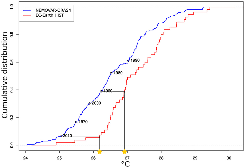
Figure 1. Example of the implementation of the quantile matching method: cumulative distribution function for the SST in one grid point of the Tropical Pacific in blue for NEMOVAR-ORAS4 and in red for a historical simulation of EC-Earth3. The circles in the reanalysis distribution indicate the value on November 1 of the year indicated in the figure. The prediction at that grid point will be initialized with the value from the historical simulation, which has the same cumulative distribution as NEMOVAR-ORAS4 at the initialization time (the yellow stars indicate the value for the start dates of 1960 and 2010). This calculation is made for all the grid points and all the ocean prognostic variables.
The ratio between the model and the reanalysis SST variance is shown in Figure 2. Regions with the highest variance mismatch (darkest colors in Figure 2) are the areas where the QM method applies larger corrections to scale the observed variability onto the model amplitude.
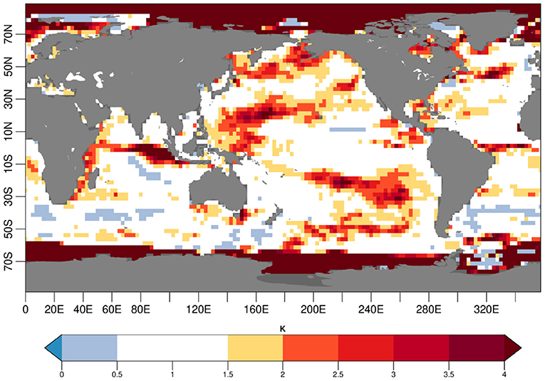
Figure 2. Ratio of SST model variance over the NEMOVAR-ORAS4 variance calculated over the November 1960–2014 start dates. The NEMOVAR-ORAS4 variance is calculated concatenating the 5 ensemble members available, while for the model one EC-Earth3 historical simulation is used.
The model in use for this study is the CMIP6 version of EC-Earth3 GCM (Döscher et al., 2021). Its atmospheric component is the European Centre for Medium-Range Weather Forecasts Integrated Forecasting System (IFS cycle cy36r4) in its standard resolution, with 91 vertical levels and a T255 horizontal resolution. The ocean component is the NEMO model version 3.6 (Madec and NEMO System Team, 2015), with ORCA1 configuration (about 1 degree with enhanced tropical resolution) and 75 vertical levels. The sea-ice component is LIM3 (Rousset et al., 2015) directly embedded into NEMO. The atmospheric and ocean components are coupled via OASIS3 (Craig et al., 2017). Information on the dynamic vegetation is prescribed from a previous simulation with LPJ-GUESS (Smith et al., 2014).
The benchmark hindcasts are a full field initialized experiment and an ensemble of 15 uninitialized CMIP6 historical simulations (Histo), assessed by Bilbao et al. (2021). All the experiments, including our QM, are carried out with the same model version. In the FFI experiment, all the variables from each model component are initialized with observational estimates (reanalysis). The atmosphere and land surface initial conditions are taken from the ERA-40 reanalysis (Uppala et al., 2005) for start dates before 1979 and ERA-Interim (Dee et al., 2011) afterwards. The ocean initial conditions are taken from the 3D-Var five-member ocean reanalysis NEMOVAR-ORAS4, while the sea-ice initial conditions are produced with a NEMO-LIM simulation driven by DFS5.2 forcing fluxes (Brodeau et al., 2009). The DFS5.2 forcing data corresponds to a corrected version of ERA-interim accounting for radiative and precipitation observations in the Arctic. The solar irradiance, volcanic and anthropogenic aerosol load, and greenhouse gas concentrations are prescribed using the CMIP6 radiative forcing estimates up to 2014. After that date, the SSP2-4.5 scenario (O'Neill et al., 2016) is used.
Both initialized experiments (FFI and QM) are composed by 10 ensemble members, initialized every November from 1960 until 2014 and running for 5 years. The ensemble is generated using perturbations in the 3-dimensional temperature field in the atmospheric component, and using the 5-member ensemble from the NEMOVAR-ORAS4 reanalysis in the ocean.
The QM is applied to the ocean component and is performed for all the ocean prognostic variables and grid points, by matching the 5 members of NEMOVAR-ORAS4 separately, in order to obtain 5 different initial conditions. The atmospheric and sea-ice components of the QM experiment have identical initial condition as the FFI.
The forecast time-dependent climatologies are computed for the longest common period (1965–2014). For each forecast year (from 1 to 5), a set of predictions is available within the 1965–2014 period (e.g., 1965 is predicted at forecast year 1 for the prediction starting in November 1964, and also as forecast year 5 for the prediction starting in November 1960). The forecast time-dependent bias is calculated as the difference between the model and the observed climatologies. The drift, i.e., the evolution of the bias with forecast time, is estimated as the difference between the first and the last forecast year climatologies for the model. This estimate of the drift provides a simplistic picture but it already highlights the main features of the model drift.
To measure the forecast quality, we use the anomaly correlation (AC) and the root mean square error (RMSE). The confidence interval is calculated with a t-distribution for the AC and with a χ2 distribution for the RMSE. The serial dependence between the hindcasts is accounted for in the computation of the confidence interval using the Von Storch and Zwiers (2001) formula. The confidence interval also takes into account the trend, that is not removed in the computation of the skill. The skill scores are computed either on annual mean values, or after smoothing the timeseries with a 1-year running mean in order to filter out seasonal climate variability and focus on interannual prediction skill. To measure the impact of the QM on the forecast quality, we compute the differences of ACs between the QM and FFI, and between QM and Histo. We use the method by Siegert et al. (2017) to identify the statistically significant differences in skill between the various experiments.
We have used several observational datasets for verification purposes: the GISTEMPv4 (Lenssen et al., 2019) NASA gridded surface temperature anomaly, the EN4 (Good et al., 2013) for the ocean heat content, and HadISST (Rayner et al., 2003) for the computation of the AMV. For the study of the initial SST bias and drift, we have used the NEMOVAR-ORAS4 reanalysis (as it represents the initial reference state for QM and the initial condition for FFI). Since observations of the full AMOC cell and the barotropic stream function are not available, they are validated against the NEMOVAR-ORAS4 reanalysis. The sea level pressure is validated against the ERA-40 and ERA-Interim reanalyses.
Initializing the predictions with a state that belongs to the model attractor implies that the mean state of the predictions is biased with respect to the observations since the beginning of the forecast. The top left panel of Figure 3 shows the SST model bias with respect to the NEMOVAR-ORAS4 reanalysis in the first forecast month. The model displays a widespread warm bias over the Tropical Pacific extending toward the extratropics in the eastern basin. An even more pronounced warm bias appears in the Southern Ocean, while the Subpolar North Atlantic region presents an intense cold bias. These features are consistent with the ones found in the bias of Histo (Supplementary Figure 1). The top right panel of Figure 3 shows the annual mean climatologies of the global SST as a function of the forecast time. Consistently with the bias map, the QM climatology (in red) results warmer than the NEMOVAR-ORAS4 climatology (black line), and remains close to the Histo climatology (in yellow) throughout the whole forecast period. In contrast, the climatology of the FFI experiment starts closer to NEMOVAR-ORAS4 but it drifts after the first forecast year. The reason for which the FFI experiment drifts away from the Histo climatologies is extensively investigated in Bilbao et al. (2021), where it is suggested to be an effect of the initial shock that leads to a collapse in Labrador Sea convection. This issue will be further discussed in section 3.3. However, the global drift toward colder temperatures is not occurring all around the globe as it is shown in the bottom right panel of Figure 3. Although a positive drift in SST is present in the Southern Ocean, the largest negative ones occur in the North Atlantic, particularly in the subpolar gyre region. Conversely, and as expected, the QM largely prevents the model drifts, with values of even an order of magnitude lower with respect to the FFI (bottom left panel of Figure 3).
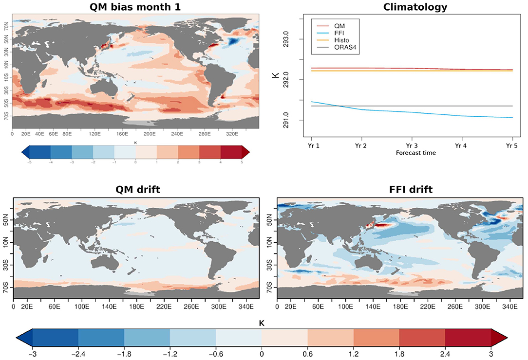
Figure 3. Top left: SST bias of the QM experiment for the first forecast month calculated against NEMOVAR-ORAS4 reanalysis. Top right: forecast time-dependent climatologies of the annual mean global SST, calculated as explained in section 2.3. The ensemble mean climatology is shown in red for QM, in blue for FFI, in yellow for Histo, and in black for NEMOVAR-ORAS4. Bottom: drift calculated as the difference between the first and the last forecast year climatologies of QM (left panel) and FFI (right panel).
We first evaluate the global skill in predicting the surface fields. The QM experiment exhibits high forecast quality in surface temperature (first column Figure 4) and sea level pressure (first column Figure 5) as indicated by the AC against the GISTEMPv4 dataset and ERA-40-ERA-Interim, shown in the first columns of Figures 4, 5, respectively. The skill in surface temperature in the first forecast year is globally significant, the main exceptions being a few regions over Asia and the Southern Ocean and a small region in the North Atlantic. At longer forecast times (2–5 forecast years), the region of non-significant skill in the North Atlantic expands, as well as in the Southern Ocean, and a new region in the central Tropical Pacific loses significance. Also the sea level pressure partly loses skill after the first forecast year and the regions with significant skill remain the subtropical gyre region in the Pacific and the Southern Ocean, which are the regions with the highest model biases during the first forecast month (Figure 3). When compared to Histo, the QM predictions show significant improvements over a predominant part of the Pacific and over the North Atlantic subpolar region (NASP) as well as the Southern Ocean, during the first forecast year for both the surface temperature (middle column Figure 4) and the sea level pressure fields (middle column Figure 5). The significant added-value with respect to Histo in the NASP surface temperature is maintained at longer forecast years (bottom panels of Figure 4). However, the improvement is partially lost at forecast years 2–5 in the zone of the inter-gyre position, where the subpolar and subtropical gyres meet. The QM also outperforms the FFI in predicting the NASP surface temperature and, more importantly, the improved skill maintains significance throughout the whole forecast time (third column Figure 4). However, analogously to what is shown in the comparison with Histo, there is a degradation of skill along the Gulf stream for the forecast years 2–5, which could potentially be due to a wrong positioning of the current in the QM predictions. Differences between QM and FFI or Histo inland temperature are marginal. The AC results are broadly consistent with the residual correlations computed according to Smith et al. (2019), which are shown in Supplementary Figure 2 of the Supplementary Material.
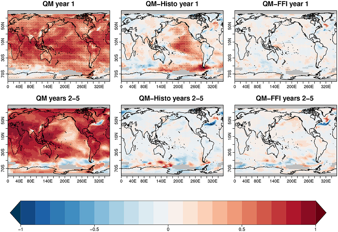
Figure 4. Anomaly correlation for the surface temperature calculated against the GISTEMPv4 dataset. The first column represents the quantile matching (QM) skill in the first forecast year (top) and the 2–5 forecast years (bottom). The middle column shows the difference between QM and Histo skill, and the third column the difference between QM and full-field initialization (FFI) skill. The black dots indicate regions of significant anomaly correlation (AC) (first column), and regions where the difference in AC is statistically significant with 95% confident level (second and third column).
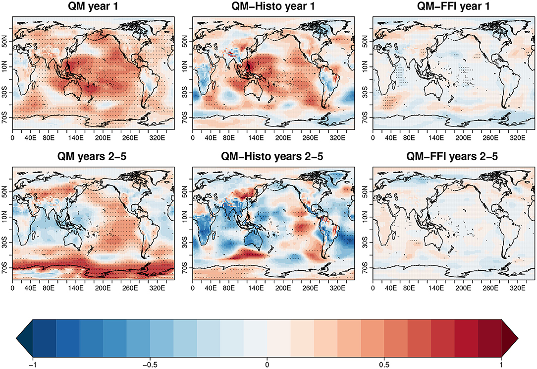
Figure 5. The same as in Figure 4, but for the sea level pressure. The anomaly correlation (AC) is calculated against ERA-40 and Era-Interim reanalysis.
The comparison of QM with FFI for the sea level pressure (third column Figure 5) highlights a statistically significant skill improvement in the Antarctic circumpolar current and a degradation of skill in the Tropical Pacific and the Indian Ocean during the first forecast year, while significance in the skill difference is lost at forecast years 2–5.
We now focus on the upper layer ocean heat content (0–300 m) because of its crucial role in the ocean meridional transport: Figure 6 shows the skill comparison between QM and Histo/FFI. Similarly to what is shown for the surface temperature, the QM significantly improves the skill in the Pacific and the NASP region with respect to Histo, although there is not a clear improvement over the Southern Ocean. Besides, skill over the Indian Ocean is improved. Part of those improvements are also maintained at longer timescales. When comparing with the FFI prediction, we find that the added value of the QM is mainly located over the NASP region, consistently with the surface temperature results.
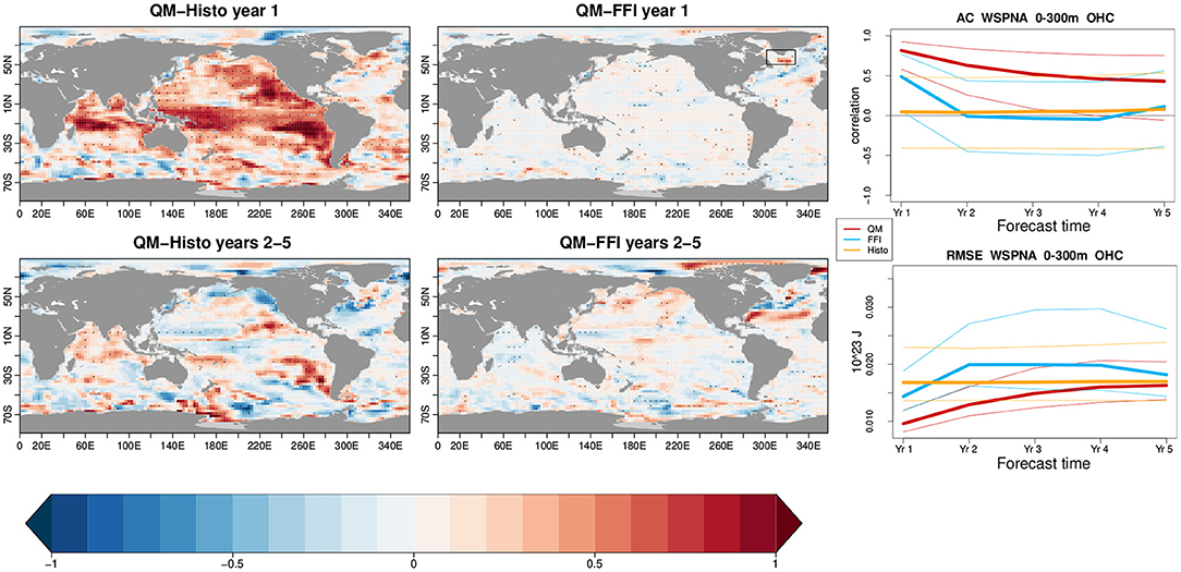
Figure 6. Skill difference in the upper 300 m ocean heat content, computed against EN4 observational dataset. The first column shows the anomaly correlation (AC) difference between quantile matching (QM) and Histo for the first forecast year (top) and the 2–5 forecast years (bottom). The second column shows the difference between QM and full-field initialization (FFI). The third column is a zoom on the regional mean of the western subpolar North Atlantic sector (WSPNA; 50–65° N, 60–30° W) as indicated by the black box. The AC and root mean square error (RMSE) are calculated with yearly mean data along the forecast time and are shown, respectively, in the top and bottom panel. In red is shown the QM experiment, in blue the FFI, and in yellow the Histo. The thin lines represent the 95% confidence interval obtained with a t-distribution for the correlation and a χ2 distribution for the RMSE.
We now zoom over the western subpolar North Atlantic region (50–65° N, 60–30° W, WSPNA), as this is a region in which SST and ocean heat content have been shown to influence the temperature and precipitation over the neighboring continents (Buckley et al., 2019). The third column of Figure 6 shows the AC (first row) and the RMSE (second row) over the WSPNA region as a function of the forecast time. The highest values of ACs and the lowest values of RMSE over the WSPNA region and during the entire forecast time are obtained with the QM (red lines). Conversely, the Histo simulations (yellow lines) do not show significant AC in any of the forecast years, whereas the FFI loses its skill after the first forecast year.
In the previous section, we have shown significant improvements in the NASP region, specifically in the Western sector of QM with respect to FFI. Bilbao et al. (2021) performed an assessment for an analogous decadal prediction experiment based on FFI, and highlighted the collapse of deep convection in the Labrador Sea with a consequent weakening of the AMOC, subsequent to initialization. This led to a lack of prediction skill for the upper ocean heat content and the surface temperature in the NASP. We therefore look at the deep convection activity in the Labrador Sea in an attempt to explain the origins of the QM skill improvements presented in the previous section. Figure 7 shows the ensemble mean of the mixed layer depth in the Labrador Sea (55–65° N, 56–46° W), as a proxy for the deep convection intensity, for the February–March–April mean, which are the months of deepest mixing. In order to better understand the behavior of the Histo simulations, we have isolated three members that show no deep convection throughout most of the historical period (top right panel of Figure 7), from the rest of the Histo ensemble (top left panel). The Histo ensemble mean with regular convection is representative of the response to external forcings only and shows lower values than the NEMOVAR-ORAS4 reference. In the experiments with FFI, deep convection collapses very quickly with forecast time (bottom right panel of Figure 7) preventing FFI to follow the NEMOVAR-ORAS4 variability, consistently with what was found by Bilbao et al. (2021). In contrast, QM (bottom left panel of Figure 7) is able to partly reproduce the variability present in NEMOVAR-ORAS4: after initialization, it shows a slight increase in convective activity during the two peaks observed in the 1980s and in the 1990s. However, this does not directly translate into an increase of forecast skill, as the QM does not improve with respect to the Histo ensemble that preserves the convection. While Histo has a constant skill throughout the whole forecast time, QM presents statistically significant AC only during the first year (top left panel of Figure 8). This is probably due to the fact that the skill in predicting the mixed layer depth is dominated by the external forcing changes that have induced an increase in stratification hindering convection activity. The additional model variability that attempts at capturing the observed one rather constitutes an additional noise, which is detrimental to the forecast performance. The results in terms of RMSE (bottom left panel of Figure 8) are consistent with what is shown by the AC.
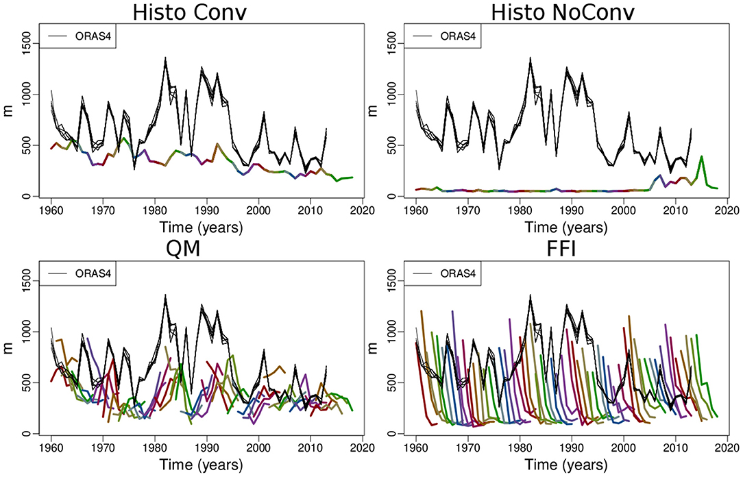
Figure 7. Evolution of the mixed layer depth ensemble mean for the February–March–April average in the Labrador Sea. The top row shows the Histo ensemble splitted into members that exhibit a regular convection activity (left), from the three which show no convection throughout most of the historical period (right). The second row shows, respectively, the QM (left) and the FFI (right) evolution. The different start dates are represented with different colors. The NEMOVAR-ORAS4 is shown in black.
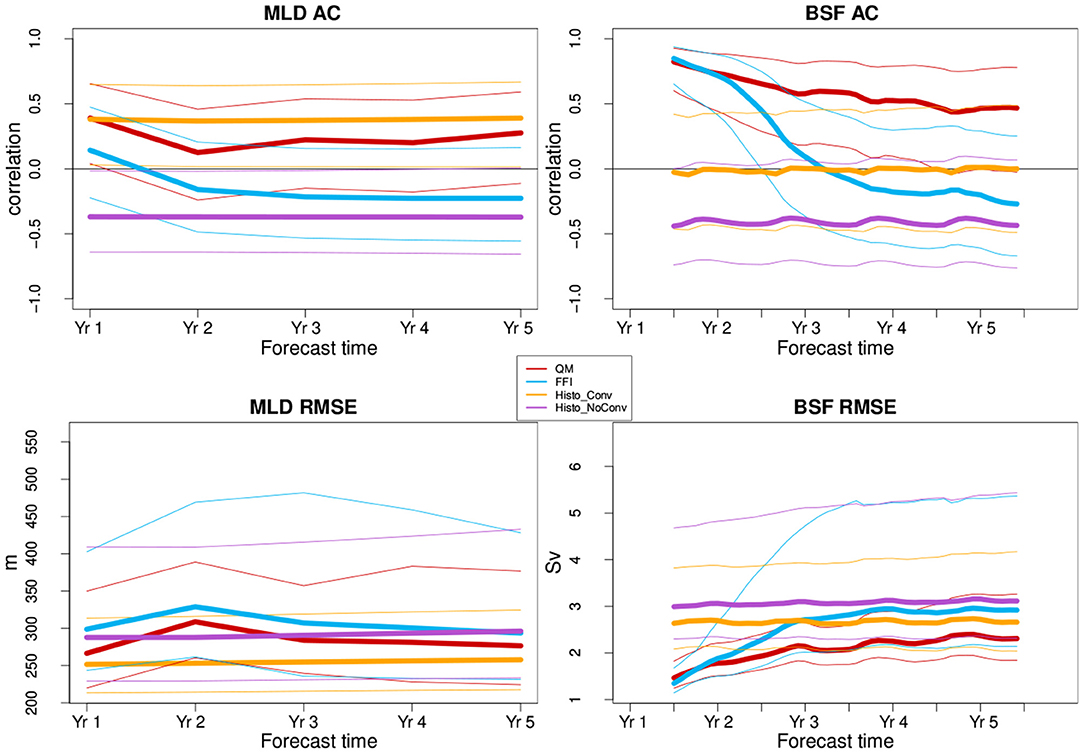
Figure 8. Anomaly correlation of the mixed layer depth (top left panel) and the barotropic stream function (top right panel) in the Labrador Sea (55–65°N, 56–46°W). The second row shows the respective root mean square error (RMSE). Quantile matching (QM) is shown in red, the full-field initialization (FFI) in blue, the Histo with convection is shown in yellow, and in purple the Histo members with no convection. The skill are computed against NEMOVAR-ORAS4, using the February–March–April mean for the mixed layer depth, and a running mean of 12 months for the barotropic stream function. The thin lines represent the 95% confidence interval obtained with a t-distribution for the correlation and a χ2 distribution for the RMSE.
We assess the skill in predicting the barotropic circulation by looking at the barotropic stream function, which characterizes the horizontal water transport integrated vertically in the Labrador Sea (right column of Figure 8). We find that Histo do not show any skill. The initialized predictions, on the other hand, have similar skill at the beginning of the forecast. However, the skill of FFI deteriorates with forecast time and is lost at forecast year 3, while the skill of QM is maintained throughout the whole forecast time.
In summary, we have shown that the QM avoids the Labrador Sea deep convection collapse that occurs in the FFI experiment, and improves the prediction skill of the barotropic stream function with respect to both the FFI and the Histo simulations. We are now interested in investigating the effect of these improvements on the AMOC. Since the AMOC skill depends on the latitude range at which it is considered, we show the results in a Hovmoller diagram of the AC (Figure 9). We have computed the AMOC index as the maximum of the Atlantic meridional overturning stream function in adjacent latitude-depth boxes of latitude range of 2 degrees (from 20° to 60° N) and depth range of 900–3,000 m depth. If we focus north of 40°N, the FFI starts with high skill that progressively deteriorates until the third forecast year down to an AC smaller than 0.1, probably due to the collapse in deep convection. This is largely improved by the QM that shows high skill in predicting the AMOC, particularly at subpolar latitudes, for the entire forecast time. The skill of FFI at lower latitudes is marginally higher than the QM one throughout the whole forecast time. One reason to explain this is that the detrimental effect of the convection collapse might need longer time to propagate at lower latitudes than the 5 years that we have available. The skill of the Histo simulations is constant with forecast time. This is consistent with the results in Borchert et al. (2021), where the good representation of the NASP SST in the CMIP6 historical simulations is attributed to the AMOC-related response to the forcings (volcanic eruptions and partly solar forcing).
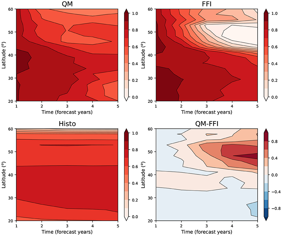
Figure 9. Hovmoller diagrams of the AMOC anomaly correlation with NEMOVAR-ORAS4. The Atlantic Meridional Overturning Circulation (AMOC) is calculated as the maximum of the Atlantic meridional overturning stream function over adjacent boxes of 2° latitude (from 20° to 60° N) and 900–3,000 m depth. The panels show, respectively, the quantile matching (QM) (top left), the full-field initialization (FFI) (top right), the Histo (bottom left), and the difference between the QM and the FFI skill (bottom right).
Finally, we complement the North Atlantic analysis with the assessment of the skill in predicting the AMV. The AMV index is calculated as the difference between the regional SST anomalies in the North Atlantic (0° to 60° N and 80° to 0° W) and the global mean SST anomalies (between 60° S and 60° N), following the definition by Trenberth and Shea (2006). The ensemble QM predictions successfully capture the observed warming trend (left panel of Figure 10). In terms of skill, both the initialized predictions and the Histo simulations succeed in predicting the AMV index with skill significantly different than 0 along the whole forecast period as shown by the confidence intervals (thin lines in Figure 10). The prediction skill of FFI starts close to the skill of Histo and it might be generated by the AMV persistence. During the first two forecast years, QM outperforms FFI, both in terms of AC and RMS (second and third panel of Figure 10), although the difference is not statistically significant.
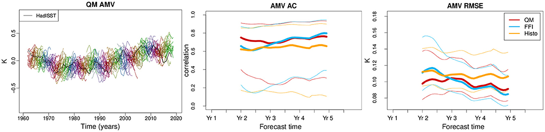
Figure 10. Atlantic multidecadal variability (AMV) index for the quantile matching (QM) predictions (left). The index computed from HadISST is shown in black. The different colors represent the different start dates. The anomaly correlation (AC) and the root mean square error (RMSE) of the AMV index are shown, respectively, in the central and right panels. The skill scores are calculated against the HadISST dataset, applying a 2-year running mean to the data. As in previous figures, the thin lines represent the 95% confidence interval obtained with a t-distribution for the correlation and a χ2 distribution for the RMSE.
In this study, we have presented a novel initialization method for decadal climate predictions, namely the quantile matching. This method aims at tackling two major issues:
• The drift coming from initializing the predictions away from the model preferred trajectories, similarly to any other anomaly initialization method;
• The potential inconsistencies between the observed/model distribution of variability.
The quantile matching method selects the initial condition of the prediction as the model state, which is identically located in the model distribution as the observed initial state in the observed distribution. Therefore, the initial state belongs to the model attractor, reducing the drift. Moreover, matching in the observed and model statistical distributions scales the observed variability toward the model one, correcting any potential amplitude incompatibilities. The forecast skill assessment of a decadal prediction with EC-Earth3, initialized with the quantile matching method, has led to the following findings:
• Surface temperature has high significant skill throughout the forecast years, in agreement with other studies (e.g., Smith et al., 2019).
• In the North Atlantic subpolar region, the quantile matching enhances the surface temperature and ocean heat content skill, compared to the historical simulations and the full field initialized predictions.
• The quantile matching avoids a collapse of deep convection in the Labrador Sea that occurred in the full field initialized predictions. This could be due to the positive effect of initializing the predictions on the model attractor. However, initialization does not seem to have a direct impact on the skill of the mixed layer depth, as no significant skill improvements are detected compared to the historical simulations. This is probably due to the fact that the skill in predicting the mixed layer depth is dominated by the trend that the historical simulations is able to capture.
• The skill of the barotropic stream function in the Western subpolar North Atlantic sector for the quantile matching predictions is significant throughout the whole forecast period and is the highest compared to both the full field initialized predictions and the historical simulations.
• The quantile matching has a positive impact on the Atlantic Meridional Overturning Circulation, which is skillfully predicted throughout the whole forecast time. The Atlantic Multidecadal Variability is well-forecasted along the whole forecast time by both the initialized predictions and the historical simulations.
The effect of the reduced prediction drift translates into an improved forecast skill of the meridional and barotropic ocean transports in the North Atlantic.
Considering that the ocean holds most of the memory in the climate system, we have performed the quantile matching on the ocean model component only. However, previous studies have highlighted the importance of having a sea-ice initial state consistent with the ocean state (Volpi et al., 2017a; Tian et al., 2020). Therefore, the use of different initialization techniques for the ocean and sea-ice components could have generated some instabilities in the quantile matching decadal predictions. A step further for this work would be performing the quantile matching also in the sea-ice model component. Besides, the use of more sophisticated atmosphere-ocean coupled initialization technique (Counillon et al., 2014; Brune and Baehr, 2020) would address the issue of the initial shock originated by the use of disjoint reanalyses for the initialization of the model components (Mulholland et al., 2015).
The raw data supporting the conclusions of this article will be made available by the authors, without undue reservation.
DV, VG, PO, and FD-R designed the quantile matching experiment. DV performed the decadal climate predictions and performed the analysis with the contributions of RB, VM, and RM. PE assisted with the settings of the workflow manager. AA contributed to the cmorizations of the outputs. RM and AA ran the benchmark simulations. PO, VG, FD-R, VM, and SC contributed to the discussion and the interpretation of the results. DV and VM prepared the manuscript with the contribution of all co-authors.
This study was supported by the project LISTEN funded by the European Commission Horizon 2020 Marie Skłodowska-Curie Actions - IF (GA 799930).
The authors declare that the research was conducted in the absence of any commercial or financial relationships that could be construed as a potential conflict of interest.
The authors thankfully acknowledge the computer resources from the ECMWF special project INCIPIT (spitvolp) and the technical assistance provided by ECMWF and BSC. The climate simulations have been performed using Autosubmit workflow manager (Manubens-Gil et al., 2016). The authors thank Paolo Davini for providing the restart files of the historical simulation used to implement the quantile matching. We acknowledge Saskia Loosveldt and the earthdiags and ESMValTool suite developers, as well as the startR and s2dverification (Manubens et al., 2018) software packages developers, as these tools were used to postprocess, analyze, and visualize the results presented in this work. PO acknowledges support by the Spanish Ministry of Economy, Industry and Competitiveness through the Ramon y Cajal grant (RYC-2017-22772).
The Supplementary Material for this article can be found online at: https://www.frontiersin.org/articles/10.3389/fclim.2021.681127/full#supplementary-material
Bellucci, A., Haarsma, R., Bellouin, N., Booth, B., Cagnazzo, C., van den Hurk, B., et al. (2015a). Advancements in decadal climate predictability: the role of nonoceanic drivers. Rev. Geophys. 53, 165–202. doi: 10.1002/2014RG000473
Bellucci, A., Haarsma, R., Gualdi, S., Athanasiadis, P. J., Caian, M., Cassou, C., et al. (2015b). An assessment of a multi-model ensemble of decadal climate predictions. Clim. Dyn. 44, 2787–2806. doi: 10.1007/s00382-014-2164-y
Beverley, J. D., Woolnough, S. J., Baker, L. H., Johnson, S. J., and Weisheimer, A. (2019). The northern hemisphere circumglobal teleconnection in a seasonal forecast model and its relationship to european summer forecast skill. Clim. Dyn. 52, 3759–3771. doi: 10.1007/s00382-018-4371-4
Bilbao, R., Wild, S., Ortega, P., Acosta-Navarro, J., Arsouze, T., Bretonniére, P.-A., et al. (2021). Assessment of a full-field initialized decadal climate prediction system with the cmip6 version of ec-earth. Earth Syst. Dyn. 12, 173–196. doi: 10.5194/esd-12-173-2021
Blanchard-Wrigglesworth, E., Bitz, C. M., and Holland, M. M. (2011). Influence of initial conditions and climate forcing on predicting Arctic sea ice. Geophys. Res. Lett. 38:L18503. doi: 10.1029/2011GL048807
Boer, G. J., Smith, D. M., Cassou, C., Doblas-Reyes, F., Danabasoglu, G., Kirtman, B., et al. (2016). The decadal climate prediction project (DCPP) contribution to CMIP6. Geosci. Model Dev. 9, 3751–3777. doi: 10.5194/gmd-9-3751-2016
Booth, B. B. B., Dunstone, N. J., Halloran, P. R., Andrews, T., and Bellouin, N. (2012). Aerosols implicated as a prime driver of twentieth-century north atlantic climate variability. Nature 484, 228–232. doi: 10.1038/nature10946
Borchert, L. F., Menary, M. B., Swingedouw, D., Sgubin, G., Hermanson, L., and Mignot, J. (2021). Improved decadal predictions of north Atlantic subpolar gyre SST in CMIP6. Geophys. Res. Lett. 48:e2020GL091307. doi: 10.1029/2020GL091307
Brasseur, G. P., and Gallardo, L. (2016). Climate services: lessons learned and future prospects. Earths Future 4, 79–89. doi: 10.1002/2015EF000338
Brodeau, L., Barnier, B., Treguier, A., Penduff, T., and Gulev, S. (2009). An ERA40-based atmospheric forcing for global ocean circulation models. Ocean Model 31, 88–104. doi: 10.1016/j.ocemod.2009.10.005
Brune, S., and Baehr, J. (2020). Preserving the coupled atmosphere-ocean feedback in initializations of decadal climate predictions. WIREs Climate Change 11:e637. doi: 10.1002/wcc.637
Buckley, M. W., DelSole, T., Lozier, M. S., and Li, L. (2019). Predictability of north Atlantic sea surface temperature and upper-ocean heat content. J. Clim. 32, 3005–3023. doi: 10.1175/JCLI-D-18-0509.1
Cassou, C., Kushnir, Y., Hawkins, E., Pirani, A., Kucharski, F., Kang, I.-S., et al. (2018). Decadal climate variability and predictability: challenges and opportunities. Bull. Am. Meteorol. Soc. 99, 479–490. doi: 10.1175/BAMS-D-16-0286.1
Corti, S., Palmer, T., Balmaseda, M., Weisheimer, A., Drijfhout, S., Dunstone, N., et al. (2015). Impact of initial conditions versus external forcing in decadal climate predictions: a sensitivity experiment. J. Clim. 28, 4454–4470. doi: 10.1175/JCLI-D-14-00671.1
Counillon, F., Bethke, I., Keenlyside, N., Bentsen, M., Bertino, L., and Zheng, F. (2014). Seasonal-to-decadal predictions with the ensemble filter and the Norwegian earth system model: a twin experiment. Tellus A Dyn. Meteorol. Oceanogr. 66:21074. doi: 10.3402/tellusa.v66.21074
Craig, A., Valcke, S., and Coquart, L. (2017). Development and performance of a new version of the oasis coupler, OASIS3-MCT_3.0. Geosci. Model Dev. 10, 3297–3308. doi: 10.5194/gmd-10-3297-2017
Day, J., Tietsche, S., Collins, M., Goessling, H.V, Guemas, Guillory, A., et al. (2015). The arctic predictability and prediction on seasonal-to-interannual timescales (apposite) data set. Geosci. Model Dev. Discuss. 10, 8809–8833. doi: 10.5194/gmdd-8-8809-2015
Dee, D. P., Uppala, S. M., Simmons, A. J. P, Berrisford, P. P., Kobayashi, S., et al. (2011). The era-interim reanalysis: configuration and performance of the data assimilation system. Q. J. R. Meteorol. Soc. 137, 553–597. doi: 10.1002/qj.828
Doblas-Reyes, F. J., Andreu-Burillo, I., Chikamoto, Y., Garcia-Serrano, J., Guemas, V., Kimoto, M., et al. (2013a). Initialized near-term regional climate change prediction. Nat. Commun. 4:1715. doi: 10.1038/ncomms2704
Doblas-Reyes, F. J., Garcia-Serrano, J., Lienert, F., Biescas, A. P., and Rodrigues, L. R. L. (2013b). Seasonal climate predictability and forecasting: status and prospects. WIREs Climate Change 4, 245–268. doi: 10.1002/wcc.217
Döscher, R., Acosta, M., Alessandri, A., Anthoni, P., Arneth, A., Arsouze, T., et al. (2021). The ec-earth3 earth system model for the climate model intercomparison project 6. Geosci. Model Dev. Discuss. 2021, 1–90. doi: 10.5194/gmd-2020-446
Dunstone, N. J., Smith, D. M., and Eade, R. (2011). Multi-year predictability of the tropical Atlantic atmosphere driven by the high latitude north Atlantic ocean. Geophys. Res. Lett. 38:L14701. doi: 10.1029/2011GL047949
Eyring, V., Bony, S., Meehl, G. A., Senior, C. A., Stevens, B., Stouffer, R. J., et al. (2016). Overview of the coupled model intercomparison project phase 6 (CMIP6) experimental design and organization. Geosci. Model Dev. 9, 1937–1958. doi: 10.5194/gmd-9-1937-2016
Fuĉkar, N. S., Volpi, D., Guemas, V., and Doblas-Reyes, F. J. (2014). A posteriori adjustment of near-term climate predictions: accounting for the drift dependence on the initial conditions. Geophys. Res. Lett. 41, 5200–5207. doi: 10.1002/2014GL060815
Gastineau, G., and Frankignoul, C. (2015). Influence of the north Atlantic SST variability on the atmospheric circulation during the twentieth century. J. Clim. 28, 1396–1416. doi: 10.1175/JCLI-D-14-00424.1
Goddard, L., Hurrell, J. W., Kirtman, B. P., Murphy, J., Stockdale, T., and Vera, C. (2012). Two time scales for the price of one (almost). Bull. Am. Meteorol. Soc. 93, 621–629. doi: 10.1175/BAMS-D-11-00220.1
Good, S. A., Martin, M. J., and Rayner, N. A. (2013). EN4: quality controlled ocean temperature and salinity profiles and monthly objective analyses with uncertainty estimates. J. Geophys. Res. Oceans 118, 6704–6716. doi: 10.1002/2013JC009067
Guemas, V., Doblas-Reyes, F. J., Andreu-Burillo, I., and Asif, M. (2013). Retrospective prediction of the global warming slowdown in the past decade. Nat. Clim. Change 3, 649–653. doi: 10.1038/nclimate1863
Hazeleger, W., Guemas, V., Wouters, B., Corti, S., Andreu-Burillo, I., Doblas-Reyes, F. J., et al. (2013). Multiyear climate predictions using two initialization strategies. Geophys. Res. Lett. 40, 1794–1798. doi: 10.1002/grl.50355
He, Y., Wang, B., Liu, M., Liu, L., Yu, Y., Liu, J., et al. (2017). Reduction of initial shock in decadal predictions using a new initialization strategy. Geophys. Res. Lett. 44, 8538–8547. doi: 10.1002/2017GL074028
Jung, T., Doblas-Reyes, F., Goessling, H., Guemas, V., Bitz, C., Buontempo, C., et al. (2015). Polar lower-latitude linkages and their role in weather and climate prediction. Bull. Am. Meteorol. Soc. 96, ES197–ES200. doi: 10.1175/BAMS-D-15-00121.1
Kharin, V., Boer, G., Merryfield, W., Scinocca, J., and Lee, W. (2012). Statistical adjustment of decadal predictions in a changing climate. Geophys. Res. Lett. 39:L19705. doi: 10.1029/2012GL052647
Kröger, J., Pohlmann, H., Sienz, F., Marotzke, J., Baehr, J., Köhl, A., et al. (2018). Full-field initialized decadal predictions with the mpi earth system model: an initial shock in the north atlantic. Clim. Dyn. 51, 2593–2608. doi: 10.1007/s00382-017-4030-1
Kushnir, Y., Scaife, A. A., Arritt, R., Balsamo, G., Boer, G., Doblas-Reyes, F., et al. (2019). Towards operational predictions of the near-term climate. Nat. Clim. Change 9, 94–101. doi: 10.1038/s41558-018-0359-7
Latif, M., and Keenlyside, N. S. (2011). A perspective on decadal climate variability and predictability. Deep Sea Res. II Top. Stud. Oceanogr. 58, 1880–1894. doi: 10.1016/j.dsr2.2010.10.066
Lenssen, N., Schmidt, G., Hansen, J., Menne, M., Persin, A., Ruedy, R., et al. (2019). Improvements in the gistemp uncertainty model. J. Geophys. Res. Atmos. 124, 6307–6326. doi: 10.1029/2018JD029522
Magnusson, L., Alonso-Balmaseda, M., Corti, S., Molteni, F., and Stockdale, T. (2013). Evaluation of forecast strategies for seasonal and decadal forecasts in presence of systematic model errors. Clim. Dyn. 41, 2393–2409. doi: 10.1007/s00382-012-1599-2
Mann, M. E., Steinman, B. A., Brouillette, D. J., and Miller, S. K. (2021). Multidecadal climate oscillations during the past millennium driven by volcanic forcing. Science 371, 1014–1019. doi: 10.1126/science.abc5810
Manubens, N., Caron, L.-P., Hunter, A., Bellprat, O., Exarchou, E., Fuĉkar, N. S., et al. (2018). An R package for climate forecast verification. Environ. Modell. Softw. 103, 29–42. doi: 10.1016/j.envsoft.2018.01.018
Manubens-Gil, D., Vegas-Regidor, J., Prodhomme, C., Mula-Valls, O., and Doblas-Reyes, F. J. (2016). “Seamless management of ensemble climate prediction experiments on hpc platforms,” in 2016 International Conference on High Performance Computing Simulation (HPCS), Innsbruck, Austria, 895–900. doi: 10.1109/HPCSim.2016.7568429
Marotzke, J., Müller, W. A., Vamborg, F. S. E., Becker, P., Cubasch, U., Feldmann, H., et al. (2016). MiKlip: a national research project on decadal climate prediction. Bull. Am. Meteorol. Soc. 97, 2379–2394. doi: 10.1175/BAMS-D-15-00184.1
Meehl, G. A., Goddard, L., Murphy, J., Stouffer, R. J., Boer, G., Danabasoglu, G., et al. (2009). Decadal prediction: can it be skillful? Bull. Am. Meteorol. Soc. 90, 1467–1486. doi: 10.1175/2009BAMS2778.1
Merryfield, W. J., Baehr, J., Batte, L., Becker, E. J., Butler, A. H., Coelho, C. A. S., et al. (2020). Current and emerging developments in subseasonal to decadal prediction. Bull. Am. Meteorol. Soc. 101, E869–E896. doi: 10.1175/BAMS-D-19-0037.1
Mignot, J., Levermann, A., and Griesel, A. (2006). A decomposition of the atlantic meridional overturning circulation into physical components using its sensitivity to vertical diffusivity. J. Phys. Oceanogr. 36, 636–650. doi: 10.1175/JPO2891.1
Mogensen, K. S., Balmaseda, M. A., and Weaver, A. (2012). The Nemovar Ocean Data Assimilation as Implemented in the ECMWF Ocean Analysis for System4. ECMWF Technical Memorandum. Reading, UK.
Mulholland, D. P., Laloyaux, P., Haines, K., and Balmaseda, M. A. (2015). Origin and impact of initialization shocks in coupled atmosphere-ocean forecasts. Mnthly Weather Rev. 143, 4631–4644. doi: 10.1175/MWR-D-15-0076.1
Nadiga, B. T., Verma, T., Weijer, W., and Urban, N. M. (2019). Enhancing skill of initialized decadal predictions using a dynamic model of drift. Geophys. Res. Lett. 46, 9991–9999. doi: 10.1029/2019GL084223
O'Neill, B. C., Tebaldi, C., van Vuuren, D. P., Eyring, V., Friedlingstein, P., Hurtt, G., et al. (2016). The scenario model intercomparison project (scenarioMIP) for CMIP6. Geosci. Model Dev. 9, 3461–3482. doi: 10.5194/gmd-9-3461-2016
Ortega, P., Mignot, J., Swingedouw, D., Sevellec, F., and Guilyardi, E. (2015). Reconciling two alternative mechanisms behind bi-decadal variability in the north Atlantic. Prog. Oceanogr. 137, 237–249. doi: 10.1016/j.pocean.2015.06.009
Otto, J., Brown, C., Buontempo, C., Doblas-Reyes, F., Jacob, D., Juckes, M., et al. (2016). Uncertainty: lessons learned for climate services. Bull. Am. Meteorol. Soc. 97, ES265–ES269. doi: 10.1175/BAMS-D-16-0173.1
Pohlmann, H., Jungclaus, J. H., Köhl, A., Stammer, D., and Marotzke, J. (2009). Initializing decadal climate predictions with the gecco oceanic synthesis: effects on the north atlantic. J. Clim. 22, 3926–3938. doi: 10.1175/2009JCLI2535.1
Pohlmann, H., Müller, W. A., Kulkarni, K., Kameswarrao, M., Matei, D., Vamborg, F. S. E., et al. (2013). Improved forecast skill in the tropics in the new miklip decadal climate predictions. Geophys. Res. Lett. 40, 5798–5802. doi: 10.1002/2013GL058051
Polkova, I., Köhl, A., and Stammer, D. (2014). Impact of initialization procedures on the predictive skill of a coupled ocean-atmosphere model. Clim. Dyn. 42, 3151–3169. doi: 10.1007/s00382-013-1969-4
Rayner, N. A., Parker, D. E., Horton, E. B., Folland, C. K., Alexander, L. V., Rowell, D. P., et al. (2003). Global analyses of sea surface temperature, sea ice, and night marine air temperature since the late nineteenth century. J. Geophys. Res. Atmos. 108:D14. doi: 10.1029/2002JD002670
Robson, J., Ortega, P., and Sutton, R. (2016). A reversal of climatic trends in the north Atlantic since 2005. Nat. Geosci. 9, 513–517. doi: 10.1038/ngeo2727
Rousset, C., Vancoppenolle, M., Madec, G., Fichefet, T., Flavoni, S., Barthélemy, A., et al. (2015). The louvain-la-neuve sea ice model lim3.6: global and regional capabilities. Geosci. Model Dev. 8, 2991–3005. doi: 10.5194/gmd-8-2991-2015
Siegert, S., Bellprat, O., Menegoz, M., Stephenson, D. B., and Doblas-Reyes, F. J. (2017). Detecting improvements in forecast correlation skill: Statistical testing and power analysis. Mnthly Weather Rev. 145, 437–450. doi: 10.1175/MWR-D-16-0037.1
Smith, B., Wårlind, D., Arneth, A., Hickler, T., Leadley, P., Siltberg, J., et al. (2014). Implications of incorporating n cycling and n limitations on primary production in an individual-based dynamic vegetation model. Biogeosciences 11, 2027–2054. doi: 10.5194/bg-11-2027-2014
Smith, D. M., Eade, R., and Pohlmann, H. (2013). A comparison of full-field and anomaly initialization for seasonal to decadal climate prediction. Clim Dyn. 41, 3325–3338. doi: 10.1007/s00382-013-1683-2
Smith, D. M., Eade, R., Scaife, A. A., Caron, L.-P., Danabasoglu, G., DelSole, T. M., et al. (2019). Robust skill of decadal climate predictions. Clim. Atmos. Sci. 2:13. doi: 10.1038/s41612-019-0071-y
Smith, T., Reynolds, R., Peterson, T., and Lawrimore, J. (2008). Improvements to noaa's historical merged land-ocean surface temperature analysis (1880-2006). J. Clim. 21, 2283–2296. doi: 10.1175/2007JCLI2100.1
Tian, T., Yang, S., Karami, M. P., Massonnet, F., Kruschke, T., and Koenigk, T. (2020). Benefits of sea ice thickness initialization for the arctic decadal climate prediction skill in ec-earth3. Geosci. Model Dev. Discuss. 2020, 1–29. doi: 10.5194/gmd-2020-331-supplement
Tietsche, S., Day, J., Guemas, V., Hurlin, W., Keeley, S., Matei, D., et al. (2014). Seasonal to interannual arctic sea ice predictability in current global climate models. Geophys. Res. Lett. 3, 1035–1043. doi: 10.1002/2013GL058755
Trenberth, K. E., and Shea, D. J. (2006). Atlantic hurricanes and natural variability in 2005. Geophys. Res. Lett. 33:L12704. doi: 10.1029/2006GL026894
Uppala, S. M., Kȧllberg, P. W., Simmons, A. J., Andrae, U., Bechtold, V. D. C., Fiorino, M., et al. (2005). The ERA-40 reanalysis. Q. J. R. Meteorol. Soc. 131, 2961–3012. doi: 10.1256/qj.04.176
Volpi, D., Guemas, V., and Doblas-Reyes (2017a). Comparison of full field and anomaly initialisation for decadal climate prediction: towards an optimal consistency between the ocean and sea-ice anomaly initialisation state. Clim. Dyn. 49, 1181–1195. doi: 10.1007/s00382-016-3373-3
Volpi, D., Guemas, V., Doblas-Reyes, F. J., Hawkins, E., and Nichols, N. (2017b). Decadal climate prediction with a refined anomaly initialisation approach. Clim. Dyn. 48, 1841–1853. doi: 10.1007/s00382-016-3176-6
Von Storch, H., and Zwiers, F. (2001). Statistical Analysis in Climate Research. Cambridge: Cambridge University Press.
Keywords: decadal climate prediction, initialization, drift, quantile matching, full field initialization
Citation: Volpi D, Meccia VL, Guemas V, Ortega P, Bilbao R, Doblas-Reyes FJ, Amaral A, Echevarria P, Mahmood R and Corti S (2021) A Novel Initialization Technique for Decadal Climate Predictions. Front. Clim. 3:681127. doi: 10.3389/fclim.2021.681127
Received: 15 March 2021; Accepted: 26 April 2021;
Published: 17 June 2021.
Edited by:
Roxy Mathew Koll, Indian Institute of Tropical Meteorology (IITM), IndiaReviewed by:
Leonard Borchert, Sorbonne Universités, FranceCopyright © 2021 Volpi, Meccia, Guemas, Ortega, Bilbao, Doblas-Reyes, Amaral, Echevarria, Mahmood and Corti. This is an open-access article distributed under the terms of the Creative Commons Attribution License (CC BY). The use, distribution or reproduction in other forums is permitted, provided the original author(s) and the copyright owner(s) are credited and that the original publication in this journal is cited, in accordance with accepted academic practice. No use, distribution or reproduction is permitted which does not comply with these terms.
*Correspondence: Danila Volpi, ZC52b2xwaUBpc2FjLmNuci5pdA==
Disclaimer: All claims expressed in this article are solely those of the authors and do not necessarily represent those of their affiliated organizations, or those of the publisher, the editors and the reviewers. Any product that may be evaluated in this article or claim that may be made by its manufacturer is not guaranteed or endorsed by the publisher.
Research integrity at Frontiers
Learn more about the work of our research integrity team to safeguard the quality of each article we publish.