A Comparative Study on the Skill of CMIP6 Models to Preserve Daily Spatial Patterns of Monsoon Rainfall Over India

1. Introduction

Every year, several countries in South Asia including India, Sri Lanka, Burma, Bangladesh, Pakistan receive heavy rainfall from the South Asian Monsoon system, roughly during the period June-September. It is caused by formation of a low-pressure region over North-western India, resulting in northward migration of the Intertropical Convergence Zone (ITCZ). Specifically in case of India, the monsoon season accounts for about 80% of the annual rainfall in about 75% of the landmass, with the exception of some regions along the south-eastern coast and the hilly north-eastern region which receive substantial pre-monsoon (April–May) and post-monsoon (October–November) rainfall. Such rainfall is extremely important for sustenance of agriculture in India, which contributes to the lives and livelihood of over a billion people (Gadgil and Gadgil, 2006). Indian monsoon is a highly complex phenomena, exhibiting significant spatial and temporal variations during its 4-month seasons, as discussed by Gadgil (2003) and Goswami and Chakravorty (2017). Indian monsoon is considered by many climate scientists to be linked to climatic phenomena in other parts of the world through teleconnections, such as El Nino-Southern Oscillation (ENSO), Indian Ocean Dipole (IOD), and Madden-Julian Oscillations (MJO). However, it is well-known that in recent decades the monsoon circulation has significantly weakened, as pointed out by Ghosh et al. (2012) and Preethi et al. (2017), while at the same time extreme rainfall events have increased, according to Roxy et al. (2017). Naturally, there is significant concern among scientists and policy-makers about how Indian monsoon may be affected in future due to worldwide climate change. For this purpose, we need reliable simulation of future climate under different scenarios.

Over the last decade, various research groups across the world have developed global climate models such as General Circulation models (GCMs) under the aegis of Coupled Model Intercomparison Project (CMIP), with the aim of studying the impacts of various natural and anthropogenic forcings on past, present and future climate. Most of these models use physics-based differential equations about energy balance and coupling between land, ocean, and atmosphere. These models simulate global climate including many geophysical variables in the past and also the future under hypothetical scenarios related to greenhouse gas concentration in the environment (Representative Concentration Pathways) and socio-economic policies adopted by different countries (Shared Socioeconomic Pathways).

Simulations of the future by any model is hard to evaluate, since the ground truth is not known. In order to estimate the reliability of the future simulations by any model, it is necessary to evaluate its simulation of the historical period, for which we do have the ground truth. Usually, some important statistical measures are calculated from the model simulations, and compared to the corresponding measures calculated from the ground truth. The accuracy of a model is based on such comparisons. Various studies focus on various statistical measures for such evaluation. Simulations by the third phase of models (CMIP3) were not very accurate due to their course resolution and failure to take into account various environmental factors, but they were improved upon by the fifth phase of the models (CMIP5). Various studies such as Sperber et al. (2013) have compared the broad spatial and temporal characteristics of simulated monsoon rainfall in Southern Asia including India, and noticed a slight improvement in some aspects, though other aspects such as teleconnections are still not represented accurately. A similar study was done for simulation of daily maximum and minimum temperature and precipitation over China by models from both families in Sun et al. (2015). However, it was pointed out by various research groups (e.g., Saha et al., 2014; Shashikanth et al., 2014; Jayasankar et al., 2015; Pattnayak et al., 2017) that these models do not represent several characteristics of Indian Monsoon very accurately in their simulations of the historically observed period, and hence their future projections are less reliable. Singh et al. (2017) found that regionalized versions of these models, often called Regional Climate Model (RCM) could not help much. Some studies like Raju and Kumar (2014) have tried to combine the CMIP5 model simulations to improve the accuracy with respect to a few statistical measures, and identified a few models as suitable for India.

The sixth phase of models (CMIP6) which have been released recently, operate at much higher spatial resolutions and take into account more small-scale or localized processes. An excellent overview of these models is provided by Eyring et al. (2016). CMIP6 models such as Wu et al. (2019) have raised hopes of researchers. Some research such as Gusain et al. (2020), have already explored the improvements in the representation of Indian Monsoon and its different characteristics in the simulations of the historical period by some of these models. The monsoon characteristics studied by Gusain et al. (2020) from these model simulations include mean seasonal precipitation across Indian landmass, seasonal climatology of daily rainfall during the June-September period over the Monsoon Zone of Central India, extreme rainfall events across the landmass, and the duration and frequency of active and break spells—an important feature of Indian monsoon denoting intra-seasonal oscillations (studied in great details by many scientists such as Rajeevan et al., 2010; Nair et al., 2018). The study found that the CMIP6 models show a greater statistical consistency with observed data than models from CMIP5 or CMIP3 families, though the spatial variations are yet to be represented accurately. Similar studies have been made for other regions affected by monsoon systems, such as China (Xin et al., 2020). This study too focuses on the representation of various characteristics of rainfall over China, such as spatial correlation between simulated and observed data, mean seasonal precipitation across Chinese landmass, inter-annual trends of seasonal precipitation, and relation between rainfall and horizontal winds.

The aim of this work is to focus on spatial distribution of daily monsoon rainfall over India. Our aim is to see if the daily distribution of rainfall as simulated by these models have any similarity with the actual daily distribution of monsoon rainfall. However, since the model simulations are not synchronized with observations on daily basis, a direct day-by-day comparison between model simulations and observations is not possible. We wish to evaluate CMIP6 models by identifying frequent spatial patterns of daily rainfall in the simulations of monsoon by these models, and comparing these patterns with those identified from observed data. Spatial patterns have generally been considered as Empirical Orthogonal Functions (EOF) in the Earth Sciences community, including for spatial analysis of Indian Monsoon, such as Suhas et al. (2013). However, a different approach was considered in the recent works by Mitra et al. (2018), where a model based on Machine Learning was used to create a binary representation of the precipitation data. This representation was used to create a few canonical spatial patterns, such that the spatial distribution (map) of rainfall on each day can be approximated using one of these patterns. Unlike EOF-based patterns, these patterns are not additive, and have both binary and real-valued representations. The binary representations are spatio-temporally coherent, and hence more comprehensive and suitable for studying different climatic variables, as done by Sharma et al. (2021). Additionally, the model is able to identify spatial clusters, i.e., compact regions on the landmass with similar intra-seasonal and inter-seasonal variation in rainfall. In this work we use the same approach to identify such canonical spatial patterns of daily rainfall and spatial clusters from monsoon rainfall data obtained from observations by India Meteorological Department (IMD) during the period 2000–2014. Next, we apply the same technique on the monsoon rainfall simulated by seven models from CMIP6 family, to identify spatial patterns and clusters from them. The patterns and clusters obtained from each of these models are compared to those obtained from the IMD observations. We define and evaluate several measures of compatibility between these patterns. On the basis of these measures, we classify the 7 CMIP6 models. It turns out that some of the models can capture the spatial patterns partially well, but not the others. None of the models are able to account for the heavy-to-extreme rainfall events. The regions of spatial homogeneity, as identified by the simulations from most of the models, are not very homogeneous with respect to the actual observations. Thus, we conclude that CMIP6 models are only somewhat accurate in reproducing daily spatial distribution of monsoon rainfall over India.

2. Materials and Methods

2.1. Datasets

In this work, we consider precipitation data over the landmass of India during the monsoon months of June-September, for the period 2000–2014. The reason for considering this period is that it is recent and relatively less well-studied in literature. We obtain ground truth data from India Meteorological Department (IMD)¹. We also collect the data related to simulation of Indian Monsoon rainfall by the following CMIP6 models: ACCESS-ESM1.5 developed by Australian Community Climate and Earth System Simulator (ACC) (see Ziehn et al., 2020 for details), Beijing Climate Center Climate System Model (BCC) (see Wu et al., 2019 for details), Canadian Earth System Model Version 5 (CAN) (see Swart et al., 2019 for details), Earth Consortium Model Version 3 (EC) (see Wyser et al., 2020 for details), Institute of Numerical Mathematics Climate Model Version 4.8 (INM) (see Volodin et al., 2018 for details), Max Plank Institute Earth System Model Version 1.2 (MPI) (see Mauritsen et al., 2019 for details), and Norwegian Climate Center Earth System Model Version 2.0 (NOR) (see Seland et al., 2020 for details).

The datasets specifically related to Indian Monsoon simulation by these models are available at https://zenodo.org/record/3873998#.X_g60dgzaUk. This dataset was created based on the study by Mishra et al. (2020). In these simulations, the precipitation data for Indian monsoon is available at a resolution of 0.25 × 0.25° (see Pai et al., 2014). For ease of computations, we coarsen them to 1 × 1° resolution using spatial averaging, following the same grid system as the widely-used dataset published by Rajeevan et al. (2006). For the ground-truth dataset also, we use the same grid structure. According to this grid system, the landmass of India consists of 357 grid-locations. For every location, we have daily rainfall data for the June-September season (122 days) of the period 2000–2014, i.e., we have totally 122 × 15 = 1, 830 days. In case of the CMIP6 models mentioned above, the years are not synchronized to the actual years, so we must limit our analysis to statistics calculated across the years for a fair comparison.

2.2. Probabilistic Graphical Model

We fit a probabilistic graphical model developed by Mitra et al. (2018) on to each of these datasets. Consider S locations and T time-points, i.e., here S = 357 and T = 1, 830. For every location s, we consider a set of neighboring locations Ω(s), which are within a distance of 1° from s along either latitudes or longitudes. We denote by X(s, t), the precipitation at any spatial location s on day t. For any day t, the vector $X(t)={\left\{X(s,t)\right\}}_{s=1}^S$ is called the spatial map or spatial distribution of rainfall on that day. Similarly for any location s, the vector $X(s)={\left\{X(s,t)\right\}}_{t=1}^T$ is called the time-series of rainfall at that location.

The model aims to find a binary representation Z(s, t) of X(s, t). Z(s, t) = 1 essentially indicates high value of rainfall at location s on day t (wet day), while Z(s, t) = 2 indicates a low value of the same (dry day). However, there is no hard threshold between high and low values. Assignment of Z(s, t) is done based on local climatology of daily rainfall at s, and also on the influence of neighboring values Z(s′, t), where s′ ∈ Ω(s) so that spatio-temporal coherence is maintained, i.e., neighboring locations are likely to have the same value of Z. Thus, for each day t during the period under consideration, we have a real-valued spatial map X(t) of rainfall as well as a binary-valued spatial map Z(t) over the geographical domain. The model assigns each day t to a cluster denoted by U(t), such that days with “similar” spatial maps are assigned to the same cluster. A cluster is represented by a binary spatial pattern denoted by θ_d which is the mode of the binary spatial maps across the constituent days of that cluster, and also by a real-valued spatial pattern denoted by θ which is the mean of the real-valued spatial maps across the constituent days. Similarly, the model assigns a spatial cluster index V(s) to each locations s, such that locations with “similar” time-series of Z-values over the entire period of T days, are assigned to the same cluster. Also, neighboring locations are likely to be assigned to the same spatial clusters, so that spatial compactness of the clusters is maintained. Just like clusters of U, each cluster of V is represented by a canonical time-series ϕ_d of binary values and ϕ of real values.

In this model, all of the variables X, Z, U, V, are considered as random variables, while θ, θ_d, ϕ, and ϕ_d are considered as unknown parameters to be estimated. First of all, we construct a probabilistic graphical model using (Z, U, V), which is shown in Figure 1. Each node of the model represents a specific random variable, such as X(s, t), Z(s, t), U(t), or V(s). Any two Z-nodes are joined by spatial edges if they are spatially adjacent, for e.g., Z(s, t) and Z(s′, t) where s′ ∈ Ω(s). Again, two Z-nodes are joined by temporal edges if they are temporally adjacent, for e.g., Z(s, t) and Z(s, t+1). Again, Z(s, t)-node and X(s, t)-node are connected by data edges. Additionally, all Z(s, t)-nodes and X(s, t)-nodes for each day t are connected to the node U(t), though in the figure U(t) is shown to be connected to Y(t), which is a dummy node representing $Y(t)=\sum _{s=1}^{S}X(s,t)$. Similarly, all Z(s, t)-nodes of each location s are connected to the corresponding V(s)-node. Each of the edges are provided with an edge potential function Ψ. The spatial edge potential functions are defined in such a way that it takes a high value when Z(s, t) = Z(s′, t), and low value otherwise. Temporal edge potentials are defined likewise. The data edge potentials between Z(s, t) and X(s, t) are defined as the PDF of a Gamma distribution on X, whose shape and scale parameters are specific to location s and the value of Z(s, t), i.e., we assume that X(s, t) ~ Gamma(α_sk, β_sk) with k = Z(s, t). This means that the rainfall at any location is modeled by a Gamma mixture distribution with two modes [as Z(s, t) is binary], one for high values and one for low values. The daily binary spatial map Z for any day t is modeled as a Bernoulli-corrupted version of the corresponding spatial pattern θ_d[U(t)]. Similarly, the binary time series Z for any location s is modeled as a Bernoulli-corrupted version of the canonical time-series ϕ_d[V(s)].

FIGURE 1

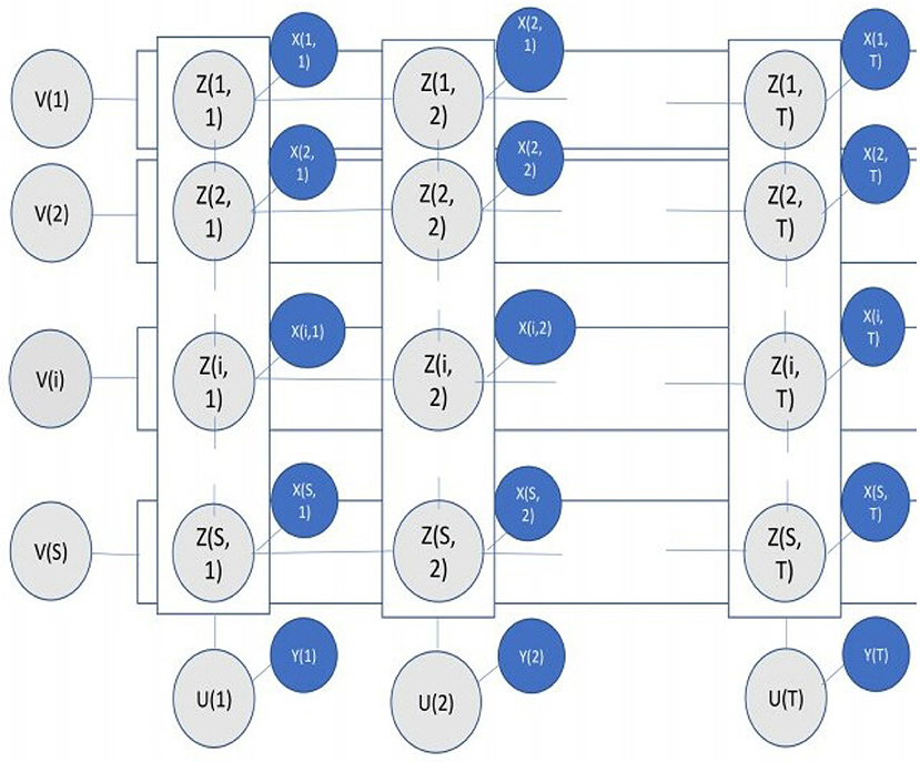
Figure 1. The probabilistic graphical model. The rows indicate spatial locations {1, S}, and the columns indicate days {1, T}. The observation nodes for X are marked in blue, while the latent variable nodes for Z, U, V are marked in gray.

This graphical model forms a Markov Random Field (Kindermann, 1980). The joint distribution P(X, Z, U, V) is the product of all the edge potentials functions. Among the random variables mentioned above, X is observed. The computation of values of (Z, U, V), is done with the aim of maximizing P(X, Z, U, V). Clearly, a configuration with more spatial and temporal coherence, will have a higher probability, due to nature of the potential functions on the spatial and temporal edges. Since standard maximum-likelihood or Expectation-Maximization are not tractable here due to the complex coupling between the variables, we use the approach of Gibbs Sampling under the paradigm of Markov Chain Monte Carlo methods (Neal, 1993). In this approach, we iteratively sample each random variable from its conditional distribution, holding all the other variables constant at their current values. The process is repeated hundreds of times, samples collected at regular intervals, and the modal values of these samples are used as Maximum A-posteriori (MAP) estimates of the random variables.

Interpretation of the values of Z, θ, θ_d, and V are important to understanding the results of this model. First of all, Z provides a binary representation of the observed data X. If we look at the spatial map of X(t) on a particular day t, then its corresponding binary representation Z(t) is a binary map where locations having high rainfall have Z(t) = 1, while those locations having low rainfall have Z(t) = 2. These binary maps are more spatially coherent than the real-valued ones, where high-rainfall and low-rainfall regions are more clearly demarcated. Coming to the spatial patterns θ, θ_d, each day's spatial map X(t) can be approximated with a real-valued θ-pattern while each day's binary spatial map Z(t) can be approximated with a binary θ_d-pattern.

The number of canonical patterns is not fixed, but estimated by the model based on the data. There are user-tuneable hyperparameters (mentioned in Mitra et al., 2018) which indicate how closely a canonical pattern must approximate the daily spatial maps/patterns, which have the effect of increasing or decreasing the number of canonical patterns. But generally about 10 patterns, each of which account for at least 60 of the 1,830 days from at least 8 of the 15 years, can cover 70–90% of the days. We call such patterns as prominent patterns, and these patterns contain the information regarding the usual daily spatial distribution of rainfall. The remaining days which are assigned to non-prominent or rare patterns are days with unusually high rainfall, spread over large parts of the country.

3. Results

Now, we come to the comparison of the different CMIP6 models with the observed data, as obtained from India Meteorological department. For this purpose, we fit the probabilistic graphical model discussed above to the daily rainfall observations X from all these datasets (observations and CMIP6 model simulations). Parameters and hyperparameters used for the model (as listed by Mitra et al., 2018) are the same for each of the datasets, for meaningful comparison. Let us denote by X^IMD, Z^IMD, θ^IMD, and ${\theta }_d^{IMD}$ the IMD observations and corresponding binary representation and spatial patterns. Similarly, we denote by X^MODEL, Z^MODEL, θ^MODEL, and ${\theta }_d^{MODEL}$ the daily rainfall values and corresponding binary representation and spatial patterns from any CMIP6 model (for specific models, we will use X^BCC, θ^NOR etc).

3.1. Quantitative Analysis of the Binary Representations

We begin our quantitative comparison of the CMIP6 model simulations and the actual observations from IMD in terms of interpreting the binary representations, i.e., Z^IMD and Z^MODEL. For each of the 357 locations, we compute the mean rainfall values across all wet days for which Z = 1 and also for all dry days for which Z = 2 separately. We also calculate the fraction of wet days (Z = 1) at each location over the study period. These indicate how wet are the wet and dry days in different locations, in the actual IMD dataset as well as in the simulations by CMIP6 models.

We denote these quantities by $n{Z}_1(s)=\frac{1}{T}\sum _{t=1}^{T}I(Z(s,t)=1)$, $X_1(s)=\frac{\sum _{t=1}^{T}X(s,t)I(Z(s,t)=1)}{\sum _{t=1}^{T}I(Z(s,t)=1)}$, $X_2(s)=\frac{\sum _{t=1}^{T}X(s,t)I(Z(s,t)=2)}{\sum _{t=1}^{T}I(Z(s,t)=2)}$ where I is the indicator function. Since these quantities are calculated at all S locations, we compare them between the model simulation datasets and the actual IMD observations using ℓ₂ norm (denoted by nZ₁ − ℓ₂, X₁ − ℓ₂, X₂ − ℓ₂) and correlation coefficient (denoted by nZ₁ − cr, X₁ − cr, X₂ − cr). The results are shown in Table 1.

TABLE 1

Table 1. The spatial statistics of X and Z, as computed from CMIP6 model simulations and compared against the IMD observations.

Another issue which we consider is spatial correlation—whether the rainfall volume at adjacent locations are correlated or not. For every pair of locations s, s′ such that s′ ∈ Ω(s), we compute the spatial correlation coefficient between the time-series X(s) and X(s′), denoted by spCr(s, s′). Similarly, we compute the spatial coherence between the binary time-series Z(s) and Z(s′), i.e., $spCh(s,s^{\prime })=\frac{1}{T}\sum _{t=1}^{T}I\left[Z(s,t)=Z(s^{\prime },t)\right]$. The mean values of these quantities are then computed over all pairs of (s, s′). These are repeated for both the IMD dataset as well the CMIP6 simulation datasets, and shown in Table 1.

It turns out that for most of the measures related to local statistics, the models BCC-CSM, EC-3, MPI-ESM-1,2, and NOR-ESM-2 perform comparable to each other, while ACC-ESM-1.5, CAN-ESM-5, and INM-CM-4.8 are found to lag behind. The spatial coherence and spatial correlation are significantly overestimated in all the models, which may indicate that only processes at larger spatial scales are simulated by these models.

3.2. Visual Analysis of Prominent Spatial Patterns

In this paper, we are specifically interested in the spatial patterns of daily rainfall, as obtained from the different CMIP6 models and from the observations. For each dataset, we identify the spatial patterns θ_d, θ as mentioned in section 2. For each dataset, we focus on the set of prominent spatial patterns, which are a subset of the spatial patterns identified by the probabilistic graphical model. As already mentioned, a prominent spatial pattern appears on at least 60 of the 1,830 days, from at least 8 of the 15 years during the study period considered. It turns out that for all datasets, there are 7–11 prominent spatial patterns.

3.2.1. IMD Dataset

The prominent patterns (binary) obtained from the IMD dataset are shown in Figure 2. There are nine prominent spatial patterns, which cover 94% of the 1,830 days in the study period. The patterns are sorted in ascending order of mean all-India rainfall, as indicated in Table 2. The first three patterns are associated with low rainfall, either scattered or limited to the North-eastern region (pattern 2) or the western coast (pattern 3). In pattern 4 too the rainfall is mostly limited to the western coast and North-east, though it is heavier magnitude. In patterns 5 and 8, the wet areas are mostly in the Gangetic plain and foot-hills of the Himalayas, while in patterns 6, 7, and 9 the rainfall is concentrated in the monsoon zone of Central India. These patterns seem to indicate that rainfall does not happen simultaneously in Gangetic plains and Central India. Although the patterns 5, 8 as well as 6, 7, 9 look nearly identical in the binary representation, they differ in the volumes of rainfall associated with them. These rainfall volumes are indicated in the real-valued versions of these prominent patterns are shown in the Supplementary Figure 1.

FIGURE 2

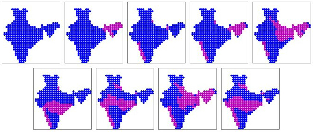
Figure 2. The nine prominent binary spatial patterns found from the observations from India Meteorological Department (IMD). Pink indicates wet locations and blue indicates dry locations. Patterns are numbered from left to right across each row, top to bottom.

TABLE 2

Table 2. Mean daily rainfall for prominent spatial patterns identified from different CMIP6 models in mm/day/location, sorted in ascending order.

3.2.2. ACCESS-ESM-1.5 Dataset

The seven prominent patterns (binary) obtained from the ACCESS simulation dataset are shown in Figure 3. The patterns are sorted according to the mean daily rainfall rates (all-India), as given in Table 2. These seven patterns cover 79% of the days. Here we find 2 patterns where most of the landmass is dry, just like the IMD dataset. In patterns 3, 4, 5, 6, 7 we find the rainfall concentrated along the western coast and the foothills of the Himalayas, North of the Gangetic planes. None of the patterns show much rainfall along major parts of the Gangetic plains, Central India and the Eastern coast. Some parts of the central India are covered in patterns 5 and 7, but simultaneously with Himalayan foothills. So many of the patterns obtained from simulations of this model do not agree well with IMD dataset. The real-valued versions of these prominent patterns are shown in Supplementary Figure 2.

FIGURE 3

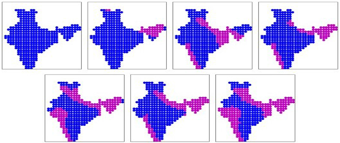
Figure 3. The seven prominent binary spatial patterns found from ACCESS-ESM-1.5 model. Pink indicates wet locations and blue indicates dry locations. Patterns are numbered from left to right across each row, top to bottom.

3.2.3. BCC-CSM Dataset

The 10 prominent patterns (binary) obtained from the BCC-CSM simulation dataset are shown in Figure 4. The patterns are sorted in ascending order of mean all-India rainfall rates, as given in Table 2. These 10 patterns cover 85% of the days. Here once again we find the first four patterns corresponding to low all-India rainfall, which are concentrated in the western coast and North-East. Pattern 5 covers the entire peninsular region including the south-eastern parts, which are known to remain dry during this period. This pattern is in disagreement with the patterns from the IMD dataset. Similarly pattern 8, which shows rainfall only in the eastern side (roughly the states of Bihar, Odisha, Bengal, and the North-east), is not found in the IMD dataset. Patterns 6, 9, 10 show rainfall in Central India, and 9, 10 include the eastern coast as well. These are broadly in agreement with the patterns 6, 7, 9 of the IMD dataset, though located a bit Northward. Pattern 7 shows rainfall in the Gangetic plain, much like patterns 5, 8 of the IMD dataset. The real-valued versions of these prominent patterns are shown in Supplementary Figure 3.

FIGURE 4

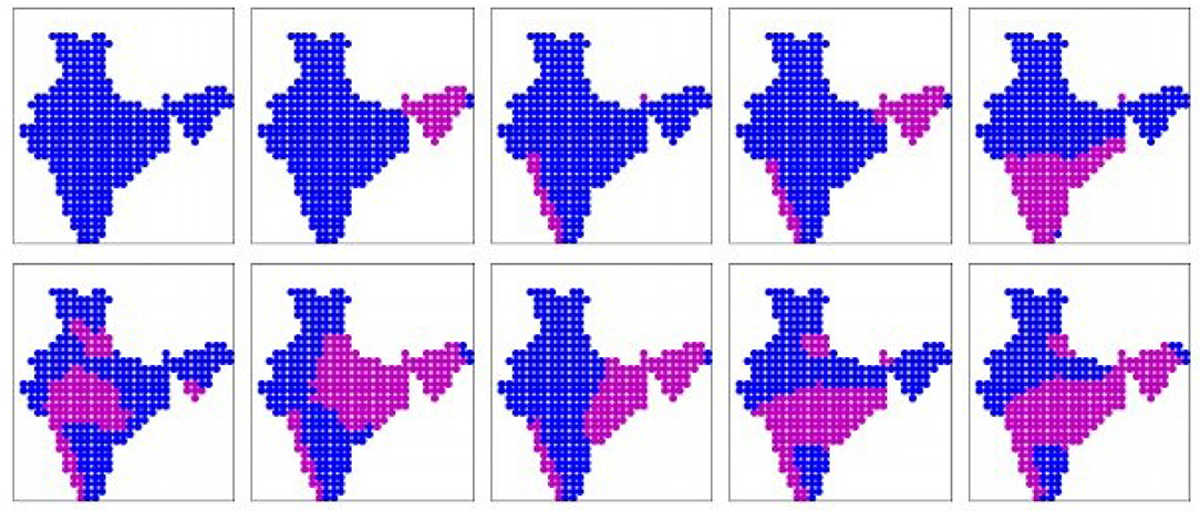
Figure 4. The 10 prominent binary spatial patterns found from BCC-CSM model. Pink indicates wet locations and blue indicates dry locations. Patterns are numbered from left to right across each row, top to bottom.

3.2.4. CAN-ESM-5 Dataset

The nine prominent patterns (binary) obtained from the CAN-ESM-5 simulation dataset are shown in Figure 5. The patterns are sorted in ascending order of mean all-India rainfall rates, as given in Table 2. These nine patterns cover 85% of the days. The patterns 1, 2, 3 resemble the corresponding dry patterns from the IMD dataset. But patterns 4, 5, 7, 8 show rainfall concentrated only in the eastern and north-eastern region, while in case of pattern 9 most of the eastern coast and the peninsular India are simultaneously wet. These patterns seem to be in disagreement with the IMD patterns. There is no pattern which covers Central India (except 9, though only partially) and western parts of the Gangetic plain including the foothills of Himalayas. The real-valued versions of these prominent patterns are shown in Supplementary Figure 4.

FIGURE 5

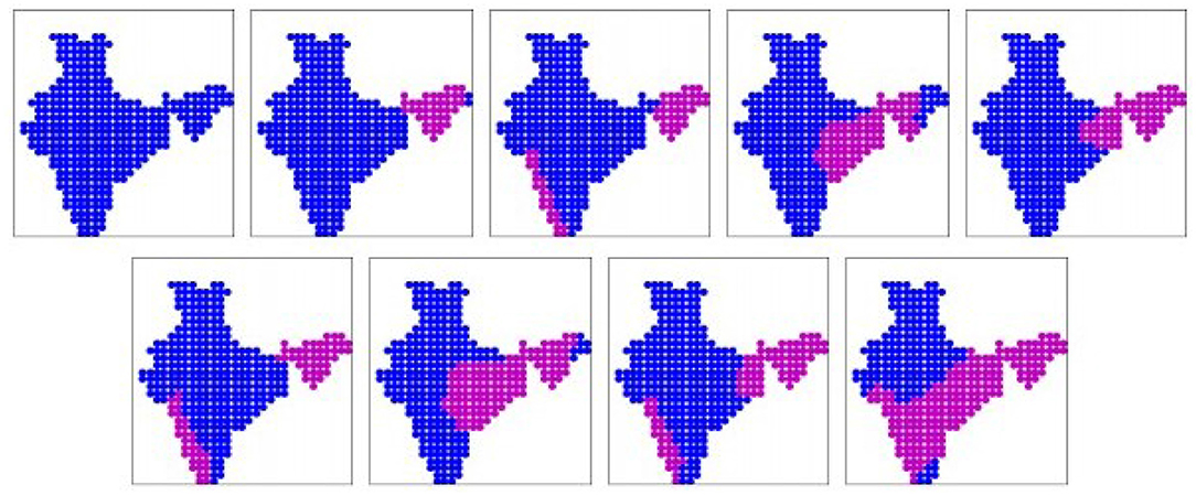
Figure 5. The nine prominent binary spatial patterns found from CAN-ESM-5 model. Pink indicates wet locations and blue indicates dry locations. Patterns are numbered from left to right across each row, top to bottom.

3.2.5. EC-3 Dataset

The nine prominent patterns (binary) obtained from the EC-3 simulation dataset are shown in Figure 6. The patterns are sorted in ascending order of mean all-India rainfall rates, as given in Table 2. These 11 patterns cover 75% of the days. Once again, patterns 1, 2, 3 show rainfall limited to the north-eastern region and western coast, like the IMD dataset. Patterns 4, 5, and 7 show rainfall over the Gangetic plain and foothills of the Himalayas, like patterns 5, 8 from the IMD dataset. But patterns 6, 8, 9 show rainfall occurring simultaneously over Central India and large parts of the Gangetic plain, which is in disagreement with the patterns from the IMD dataset. The real-valued versions of these prominent patterns are shown in Supplementary Figure 5.

FIGURE 6

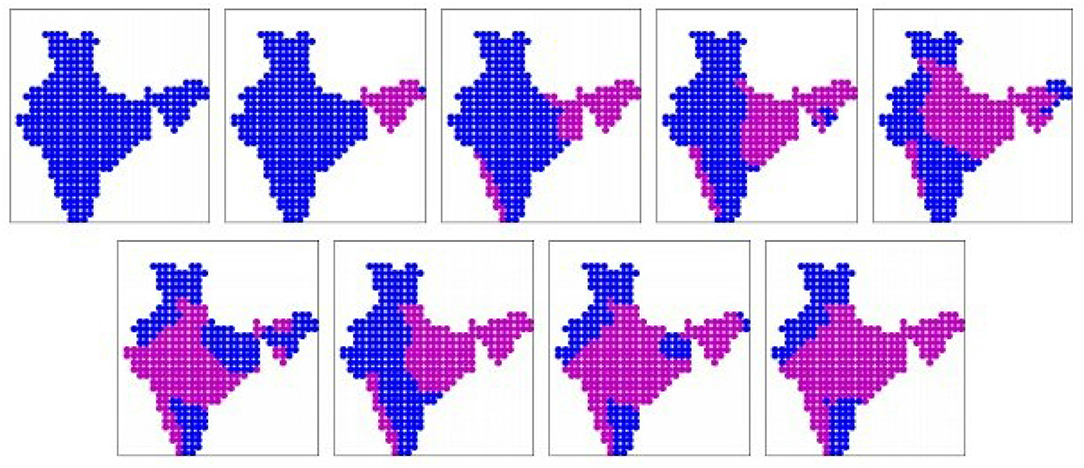
Figure 6. The nine prominent binary spatial patterns found from EC-3 model. Pink indicates wet locations and blue indicates dry locations. Patterns are numbered from left to right across each row, top to bottom.

3.2.6. INM-CM-4.8 Dataset

The 11 prominent patterns (binary) obtained from the INM-CM-4.8 simulation dataset are shown in Figure 7. The patterns are sorted in ascending order of mean all-India rainfall rates, as given in Table 2. These 11 patterns cover 82% of the days. Here we have dry patterns 1, 2, 3 like all other datasets. Pattern 5 shows rainfall over the Gangetic plain, while patterns 6, 11 shows rainfall over Central India, like the patterns from the IMD dataset. However, patterns 7 shows rainfall along the entire eastern coast, which is not observed in the IMD dataset. In patterns 4, 5, 8, 9, 10 we see rainfall simultaneously in Central India and the Gangetic plain, which too is in disagreement with the IMD patterns. The real-valued versions of these prominent patterns are shown in Supplementary Figure 6.

FIGURE 7

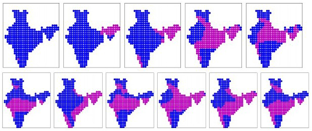
Figure 7. The 11 prominent binary spatial patterns found from INM-CM-4.8 model. Pink indicates wet locations and blue indicates dry locations. Patterns are numbered from left to right across each row, top to bottom.

3.2.7. MPI-ESM-1.2 Dataset

The nine prominent patterns (binary) obtained from the MPI-ESM-1.2 simulation dataset are shown in Figure 8. The patterns are sorted in ascending order of mean all-India rainfall rates, as given in Table 2. These nine patterns cover 75% of the days. Just like all other datasets, we have 3 dry patterns, but unlike other models, none of them show rainfall along the Western coast only. Patterns 6 and 9 show rainfall mostly over the Gangetic plain, like patterns 5, 8 from the IMD dataset. Pattern 8 shows rainfall over central India. But pattern 4 where the rainfall is over peninsular India only, as well as patterns 5,7 where the rainfall occurs from eastern coast (around Odisha state) till western parts of the Gangetic plains excluding the eastern parts of the Gangetic plain, are in disagreement with the IMD dataset. The real-valued versions of these prominent patterns are shown in Supplementary Figure 7.

FIGURE 8

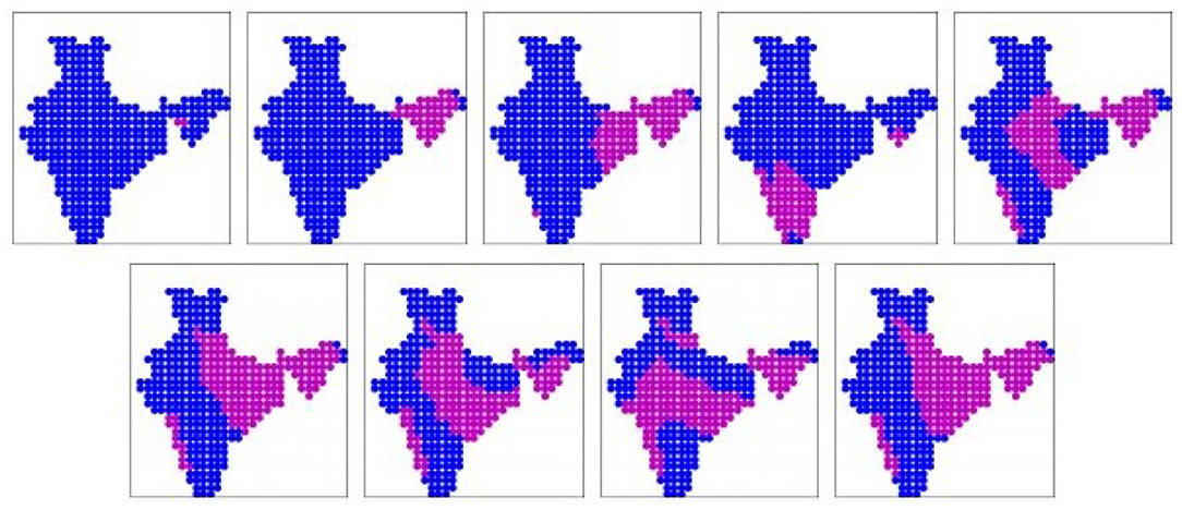
Figure 8. The nine prominent binary spatial patterns found from MPI-ESM-1.2 model. Pink indicates wet locations and blue indicates dry locations. Patterns are numbered from left to right across each row, top to bottom.

3.2.8. NOR-ESM-2 Dataset

The 10 prominent patterns (binary) obtained from the NOR-ESM-2 simulation dataset are shown in Figure 9. The patterns are sorted in ascending order of mean all-India rainfall rates, as given in Table 2. These 10 patterns cover 76% of the days. Here too we have three dry patterns like the IMD dataset. Patterns 5,8,9 show rainfall over the Gangetic plains including Himalayan foothills. However, pattern 4 which show rainfall over the Eastern region only, and patterns 6 and 10 where rainfall covers Central India and Gangetic plain simultaneously, are in disagreement with the patterns from the IMD dataset. The real-valued versions of these prominent patterns are shown in Supplementary Figure 8.

FIGURE 9

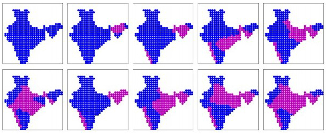
Figure 9. The 10 prominent binary spatial patterns found from NOR-ESM2 model. Pink indicates wet locations and blue indicates dry locations. Patterns are numbered from left to right across each row, top to bottom.

3.3. Quantitative Analysis of Prominent Spatial Patterns

We now carry out a quantitative analysis of the spatial patterns obtained from the different CMIP6 models and the ground truth data. The first analysis is to see how well the spatial patterns from each CMIP6 model can fit the ground truth data. For each day, we choose among the prominent spatial patterns from a particular CMIP6 model, that pattern which is the closest approximation of the spatial maps X_IMD(t) and Z_IMD(t). For this we calculate τ^MODEL(t) = min||X^IMD(t) − θ^MODEL|| and ${\tau }_d^{MODEL}(t)=min\left|\right|Z^{IMD}(t)-{\theta }_d^{MODEL}\left|\right|$, where || denotes a suitable distance measure. We use ℓ₂ norm for τ and Hamming distance for τ_d. We take the mean value of τ^MODEL and ${\tau }_d^{MODEL}$ over all the days, and denote these by PatternScore and dPatternScore. This essentially indicates, how well the prominent spatial patterns identified from the models can describe actual spatial maps of daily rainfall.

Analogously, for each day's rainfall map X^MODEL as simulated by the models, we try to approximate them with the prominent spatial patterns identified from the IMD dataset. For each simulated day, we calculate κ^MODEL(t) = min||X^MODEL(t) − θ^IMD|| and ${\kappa }_d^{MODEL}(t)=min\left|\right|Z^{MODEL}(t)-{\theta }_d^{IMD}\left|\right|$, where || denotes a suitable distance measure. We use ℓ₂ norm for X and Hamming distance for Z. We take the mean value of κ and κ_d over all the simulated days, and denote it by MapScore and dMapScore. This essentially indicates how well the daily spatial maps simulated by the models can resemble the prominent spatial patterns identified from the actual data.

The results may be seen in Table 3. We find that for the IMD dataset, dPatternScore is 0.81, which means that on any day during the study period, the binarized rainfall agrees with value predicted by the corresponding spatial pattern (binary) at about 81% of the locations on average. For other models, this score is somewhat lesser. The same trend holds when we consider PatternScore, where the actual rainfall values at each location are compared to that predicted by the corresponding spatial pattern. This indicates that the CMIP6 models have not been very effective in recognizing that there exist spatial patterns of daily rainfall. Not only do the patterns extracted from the simulation datasets not resemble those obtained from the IMD dataset, in fact the patterns are not very pronounced in their own rainfall maps.

TABLE 3

Table 3. Quantitative comparison of the spatial patterns and daily rainfall maps obtained from the IMD dataset and those obtained from different CMIP6 model simulations.

When we consider the daily spatial maps of rainfall as simulated by the models, we see somewhat unexpected results. We find that ACCESS-ESM-1.5 and CAN-ESM-5 models, which have generally been less accurate, return the least values of MapScore, indicating that the daily rainfall maps simulated by them resemble the actual spatial patterns (obtained from the real data) better, compared to other models. In fact, the MapScore is worst from the IMD dataset itself. Yet, on deeper investigation, we realize that this is due to the presence of many more extreme rainfall events in the real dataset than those simulated by the models, as shown in Table 4. We find that CAN-ESM-5 model has the least number of rainfall events above 50 mm, while for NOR-ESM-2 this number is the highest, and closest to the actual number. The real-valued spatial patterns (θ) do not contain high values of rainfall, due to which the ℓ₂ norms used for calculation of MapScore is high.

TABLE 4

Table 4. The number of extreme rainfall events in different datasets, i.e., the number of (location, day) pairs at which the volume of rainfall exceeds thresholds as mentioned in the leftmost column.

3.4. Analysis of Spatial Clusters

Now, we turn our attention to the spatial clusters obtained from the V-variable of the probabilistic graphical model. All locations assigned the same value of V constitute a spatial cluster, implying that their rainfall time-series are nearly identical. The number of spatial clusters is not fixed by the user, but determined by the model from the data. The maps showing the spatial clusters may be seen in Figure 10, where each cluster is indicated with a different color. It may be observed that all the spatial clusters obtained are spatially contiguous. The number of clusters, as indicated in Table 5, varies in the range 32–55. We find that in all cases, certain geographically special regions such as the Thar desert and the Rann of Kutch in the west, come as single clusters. In case of the clustering obtained from IMD dataset, the rain shadow region of the Deccan plateau in the south comes as a single cluster, though this feature does not show up in other models.

FIGURE 10

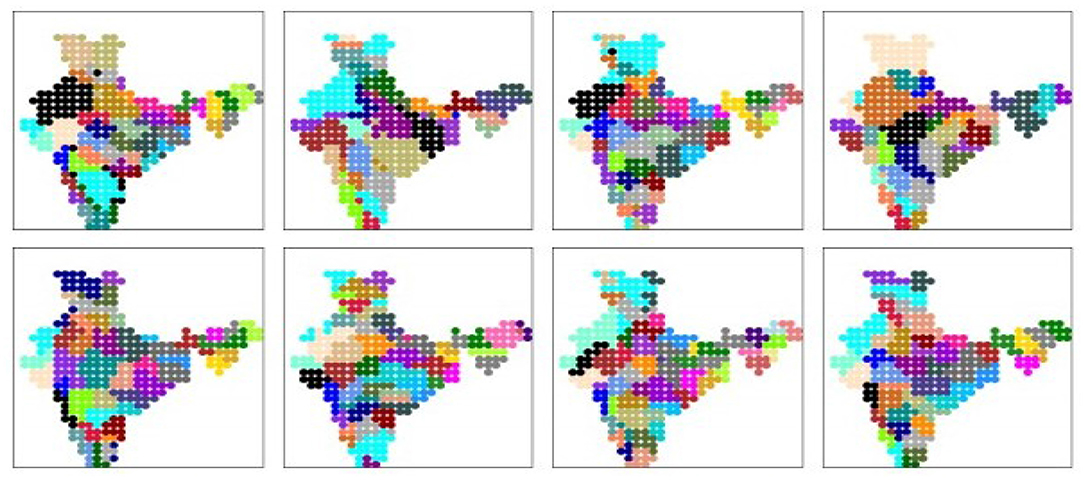
Figure 10. The spatial clusters obtained from IMD dataset and all CMIP6 model simulation datasets. Each color denotes one cluster. (Top) (left to right): IMD dataset, ACCESS-ESM-1.5, BCC-CSM, CAN-ESM-5; (Bottom) (left to right): EC-3, INM-CM-4.8, MPI-ESM-1.2, NOR-ESM-2.

TABLE 5

Table 5. Statistics of the spatial clusters computed from the IMD dataset and different CMIP6 model simulations, as mentioned in section 3.4.

Now, we investigate the quality of these spatial clusters. A cluster is useful only if it is homogeneous. For any cluster k, we calculate the mean time-series $X_k^{MODEL}$ of rainfall. We then calculate the correlation coefficients between $X_k^{MODEL}$ and the rainfall time-series X^MODEL(s) for each location s within that cluster, i.e., V^MODEL(s) = k, which indicates how well the rainfall time-series at each location is correlated to that of its spatial cluster. We take the mean of these correlation coefficients for all locations and refer to it as model-smoothness. This process is repeated for all the datasets, including IMD and CMIP6 simulations. Next, we examine if the spatial clusters obtained from the CMIP6 model simulations make any physical sense, i.e., are those regions homogeneous with respect to actual rainfall data? For this purpose, we repeat the same exercise as above using X^IMD as rainfall time-series, but V^MODEL to define the clusters, for each model separately. We call these statistics as data-smoothness.

These statistics are available in Table 5. We find that some models like ACCESS-ESM-1.5 and CAN-ESM-5 produce significantly less number of spatial clusters than the IMD dataset. The values of model-smoothness indicate that clusters from all datasets are relatively homogeneous. However, there may not be a strong physical basis of the spatial clusters obtained from the CMIP6 models, as the data-smoothness values from them are relatively low compared to that from the IMD dataset. The numbers are particularly poor for ACCESS-ESM-1.5 and CAN-ESM-5 models, and relatively better for MPI-ESM-1.2.

4. Discussions

Finally, we come to a discussion of the results. First of all, a major observation is that spatial correlation of monsoon rainfall is heavily overestimated in all the CMIP6 models, indicating that rainfall is spatially smoother in the model simulations than in the actual data. This may indicate that the models simulate monsoon rainfall through large-scale processes which cover many grids, leading to such spatial correlation. They may be missing out on localized convective events, or missing out on spatial heterogeneity of large-scale processes during monsoon. It turns out that the probabilistic graphical model is able to identify a small number (7–11) or prominent spatial patterns from each of the datasets including the IMD observations and the CMIP6 simulations. However, there are two major differences: (i) While the rainfall maps on a large fraction of the days conform to any of these prominent spatial patterns in case of the IMD dataset, this fraction is less in case of all the CMIP6 model simulations; (ii) The spatial patterns identified from the model simulations do not match well with those from the IMD dataset, and hence these model-based patterns cannot fit the spatial maps of actual daily rainfall. The second point is made based on both the visual inspection of section 3.2 and the quantitative analysis of section 3.3 using the PatternScore and dPatternScore measures. Additionally, we also see that most of the models seriously underestimate the number of extreme rainfall events. Coming to spatial clusters, we can find a number of reasonably homogeneous spatial clusters from the IMD datasets as well as from the CMIP6 model simulations, but most of the clusters formed by models do not seem to have a strong physical basis, as they are not very homogeneous with respect to actual rainfall from IMD observations, as indicated by the data-smoothness measure.

Among the different CMIP6 models we considered, we find that there is a variation in performance. The ACCESS-ESM-1.5 and CAN-ESM-5 are found to be unsuitable on almost all the measures we considered, including the spatial statistics (Table 1), number of extreme events, and suitability of their spatial patterns and spatial clusters to actual rainfall data. INM-CM-4.8 is found to perform poorly on some measures, especially the local statistics and number of extreme events, but decently on other measures. Several of the spatial patterns identified from this model are in disagreement with the spatial patterns from IMD dataset, but this is somehow not captured by the dPatternScore measure where INM-CM-4.8 does well. But the other models, namely BCC-CSM, EC-3, MPI-ESM-1.2, and NOR-ESM-2 are found to be quite robust on most of the measures that we consider.

More than hindcasting of historical data, the biggest utility of these GCMs is in simulation of future climate. It is well-known that no individual model is reliable enough for simulations, which is why multi-model ensembles are considered for most studies regarding simulation of future scenarios. However, it is important to assign weights to the ensemble members based on their performance on the historical period, since that can be evaluated against ground truth. We hope this work will enable such weighing of climate models, especially for studies about spatial properties of Indian monsoon under future scenarios.

Data Availability Statement

The datasets used in this study are all available in public domain. The observational dataset provided by India Meteorological Department are available at: https://imdpune.gov.in/Clim_Pred_LRF_New/Grided_Data_Download.html. The datasets simulated by different CMIP6 models are available at: https://zenodo.org/record/3873998#.X_g60dgzaUk.

Author Contributions

The problem formulation, experimentation, and writing of the paper were all done by AM.

Funding

This research was partially funded by Grant Number IIT/SRIC/AI/STF/2020-2021/067, provided by Sponsored Research and Industrial Consultancy (SRIC), Indian Institute of Technology Kharagpur.

Conflict of Interest

The author declares that the research was conducted in the absence of any commercial or financial relationships that could be construed as a potential conflict of interest.

Supplementary Material

The Supplementary Material for this article can be found online at: https://www.frontiersin.org/articles/10.3389/fclim.2021.654763/full#supplementary-material

Footnotes

1. ^https://imdpune.gov.in/Clim_Pred_LRF_New/Grided_Data_Download.html.

References

Eyring, V., Bony, S., Meehl, G. A., Senior, C. A., Stevens, B., Stouffer, R. J., et al. (2016). Overview of the coupled model intercomparison project phase 6 (CMIP6) experimental design and organization. Geosci. Model Dev. 9, 1937–1958. doi: 10.5194/gmd-9-1937-2016

CrossRef Full Text | Google Scholar

Gadgil, S. (2003). The Indian monsoon and its variability. Annu. Rev. Earth Planet. Sci. 31, 429–467. doi: 10.1146/annurev.earth.31.100901.141251

CrossRef Full Text | Google Scholar

Gadgil, S., and Gadgil, S. (2006). The Indian monsoon, GDP and agriculture. Econ. Polit. Week. 4887–4895. Available online at: http://www.jstor.org/stable/4418949

Google Scholar

Ghosh, S., Das, D., Kao, S.-C., and Ganguly, A. R. (2012). Lack of uniform trends but increasing spatial variability in observed Indian rainfall extremes. Nat. Clim. Change 2, 86–91. doi: 10.1038/nclimate1327

CrossRef Full Text | Google Scholar

Goswami, B., and Chakravorty, S. (2017). “Dynamics of the Indian summer monsoon climate,” in Oxford Research Encyclopedia of Climate Science. doi: 10.1093/acrefore/9780190228620.013.613

CrossRef Full Text | Google Scholar

Gusain, A., Ghosh, S., and Karmakar, S. (2020). Added value of CMIP6 over CMIP5 models in simulating Indian summer monsoon rainfall. Atmos. Res. 232:104680. doi: 10.1016/j.atmosres.2019.104680

CrossRef Full Text | Google Scholar

Jayasankar, C., Surendran, S., and Rajendran, K. (2015). Robust signals of future projections of Indian summer monsoon rainfall by IPCC AR5 climate models: role of seasonal cycle and interannual variability. Geophys. Res. Lett. 42, 3513–3520. doi: 10.1002/2015GL063659

CrossRef Full Text | Google Scholar

Kindermann, R. (1980). Markov Random Fields and Their Applications. Providence, RI: American Mathematical Society. doi: 10.1090/conm/001

CrossRef Full Text | Google Scholar

Mauritsen, T., Bader, J., Becker, T., Behrens, J., Bittner, M., Brokopf, R., et al. (2019). Developments in the MPI-M earth system model version 1.2 (MPI-ESM1. 2) and its response to increasing CO2. J. Adv. Model. Earth Syst. 11, 998–1038. doi: 10.1029/2018MS001400

PubMed Abstract | CrossRef Full Text | Google Scholar

Mishra, V., Bhatia, U., and Tiwari, A. D. (2020). Bias-corrected climate projections for South Asia from coupled model intercomparison project-6. Sci. Data 7:338. doi: 10.1038/s41597-020-00681-1

PubMed Abstract | CrossRef Full Text | Google Scholar

Mitra, A., Apte, A., Govindarajan, R., Vasan, V., and Vadlamani, S. (2018). A discrete view of the Indian monsoon to identify spatial patterns of rainfall. Dyn. Stat. Clim. Syst. 3:dzy009. doi: 10.1093/climsys/dzy009

CrossRef Full Text | Google Scholar

Nair, P., Chakraborty, A., Varikoden, H., Francis, P., and Kuttippurath, J. (2018). The local and global climate forcings induced inhomogeneity of Indian rainfall. Sci. Rep. 8, 1–12. doi: 10.1038/s41598-018-24021-x

PubMed Abstract | CrossRef Full Text | Google Scholar

Neal, R. M. (1993). Probabilistic Inference Using Markov Chain Monte Carlo Methods. Toronto, ON: Department of Computer Science; University of Toronto.

Google Scholar

Pai, D., Sridhar, L., Rajeevan, M., Sreejith, O., Satbhai, N., and Mukhopadhyay, B. (2014). Development of a new high spatial resolution (0.25 × 0.25) long period (1901–2010) daily gridded rainfall data set over India and its comparison with existing data sets over the region. Mausam 65, 1–18. Available online at: https://metnet.imd.gov.in/mausamdocs/16511_F.pdf

Google Scholar

Pattnayak, K., Kar, S., Dalal, M., and Pattnayak, R. (2017). Projections of annual rainfall and surface temperature from CMIP5 models over the BIMSTEC countries. Glob. Planet. Change 152, 152–166. doi: 10.1016/j.gloplacha.2017.03.005

CrossRef Full Text | Google Scholar

Preethi, B., Mujumdar, M., Kripalani, R., Prabhu, A., and Krishnan, R. (2017). Recent trends and tele-connections among south and East Asian summer monsoons in a warming environment. Clim. Dyn. 48, 2489–2505. doi: 10.1007/s00382-016-3218-0

CrossRef Full Text | Google Scholar

Rajeevan, M., Bhate, J., Kale, J., and Lal, B. (2006). High resolution daily gridded rainfall data for the Indian region: analysis of break and active. Curr. Sci. 91, 296–306. Available online at: https://www.jstor.org/stable/24094135

Google Scholar

Rajeevan, M., Gadgil, S., and Bhate, J. (2010). Active and break spells of the Indian summer monsoon. J. Earth Syst. Sci. 119, 229–247. doi: 10.1007/s12040-010-0019-4

CrossRef Full Text | Google Scholar

Raju, K. S., and Kumar, D. N. (2014). Ranking of global climate models for India using multicriterion analysis. Clim. Res. 60, 103–117. doi: 10.3354/cr01222

CrossRef Full Text | Google Scholar

Roxy, M. K., Ghosh, S., Pathak, A., Athulya, R., Mujumdar, M., Murtugudde, R., et al. (2017). A threefold rise in widespread extreme rain events over central India. Nat. Commun. 8, 1–11. doi: 10.1038/s41467-017-00744-9

PubMed Abstract | CrossRef Full Text | Google Scholar

Saha, A., Ghosh, S., Sahana, A., and Rao, E. (2014). Failure of CMIP5 climate models in simulating post-1950 decreasing trend of Indian monsoon. Geophys. Res. Lett. 41, 7323–7330. doi: 10.1002/2014GL061573

CrossRef Full Text | Google Scholar

Seland, Ø., Bensten, M., Graff, L., Olivié, D., Toniazzo, T., Gjermundsen, A., et al. (2020). The Norwegian earth system model, NORESM2-evaluation of the CMIP6 deck and historical simulations. Geosci. Model Dev. Discuss. 13, 6165–6200. doi: 10.5194/gmd-13-6165-2020

CrossRef Full Text

Sharma, A., Mitra, A., Vasan, V., and Govindarajan, R. (2021). Spatio-temporal relationships between rainfall and convective clouds during Indian monsoon through a discrete lens. Int. J. Climatol. 41, 1351–1368. doi: 10.1002/joc.6812

CrossRef Full Text | Google Scholar

Shashikanth, K., Salvi, K., Ghosh, S., and Rajendran, K. (2014). Do CMIP5 simulations of Indian summer monsoon rainfall differ from those of CMIP3? Atmosph. Sci. Lett. 15, 79–85. doi: 10.1002/asl2.466

CrossRef Full Text | Google Scholar

Singh, S., Ghosh, S., Sahana, A., Vittal, H., and Karmakar, S. (2017). Do dynamic regional models add value to the global model projections of indian monsoon? Clim. Dyn. 48, 1375–1397. doi: 10.1007/s00382-016-3147-y

CrossRef Full Text | Google Scholar

Sperber, K., Annamalai, H., Kang, I.-S., Kitoh, A., Moise, A., Turner, A., et al. (2013). The Asian summer monsoon: an intercomparison of CMIP5 vs. CMIP3 simulations of the late 20th century. Clim. Dyn. 41, 2711–2744. doi: 10.1007/s00382-012-1607-6

CrossRef Full Text | Google Scholar

Suhas, E., Neena, J., and Goswami, B. (2013). An Indian monsoon intraseasonal oscillations (miso) index for real time monitoring and forecast verification. Clim. Dyn. 40, 2605–2616. doi: 10.1007/s00382-012-1462-5

CrossRef Full Text | Google Scholar

Sun, Q., Miao, C., and Duan, Q. (2015). Comparative analysis of CMIP3 and CMIP5 global climate models for simulating the daily mean, maximum, and minimum temperatures and daily precipitation over China. J. Geophys. Res. 120, 4806–4824. doi: 10.1002/2014JD022994

CrossRef Full Text | Google Scholar

Swart, N. C., Cole, J. N., Kharin, V. V., Lazare, M., Scinocca, J. F., Gillett, N. P., et al. (2019). The Canadian earth system model version 5 (CANESM5. 0.3). Geosci. Model Dev. 12, 4823–4873. doi: 10.5194/gmd-12-4823-2019

CrossRef Full Text | Google Scholar

Volodin, E. M., Mortikov, E. V., Kostrykin, S. V., Galin, V. Y., Lykossov, V. N., Gritsun, A. S., et al. (2018). Simulation of the modern climate using the INM-CM48 climate model. Russ. J. Numer. Anal. Math. Model. 33, 367–374. doi: 10.1515/rnam-2018-0032

CrossRef Full Text

Wu, T., Lu, Y., Fang, Y., Xin, X., Li, L., Li, W., et al. (2019). The Beijing climate center climate system model (BCC-CSM): The main progress from CMIP5 to CMIP6. Geosci. Model Dev. 12, 1573–1600. doi: 10.5194/gmd-12-1573-2019

CrossRef Full Text | Google Scholar

Wyser, K., Noije, T. V., Yang, S., Hardenberg, J. V., O'Donnell, D., and Döscher, R. (2020). On the increased climate sensitivity in the ec-earth model from CMIP5 to CMIP6. Geosci. Model Dev. 13, 3465–3474. doi: 10.5194/gmd-13-3465-2020

CrossRef Full Text | Google Scholar

Xin, X., Wu, T., Zhang, J., Yao, J., and Fang, Y. (2020). Comparison of CMIP6 and CMIP5 simulations of precipitation in China and the East Asian summer monsoon. Int. J. Climatol. 40, 6423–6440. doi: 10.1002/joc.6590

CrossRef Full Text | Google Scholar

Ziehn, T., Chamberlain, M. A., Law, R. M., Lenton, A., Bodman, R. W., Dix, M., et al. (2020). The Australian earth system model: access-ESM1. 5. J. South. Hemis. Earth Syst. Sci. 70, 193–214. doi: 10.1071/ES19035

CrossRef Full Text | Google Scholar