Optimization of Coastal Protections in the Presence of Climate Change

It is generally acknowledged that interdependent critical infrastructure in coastal urban areas is constantly threatened by storm-induced flooding. Due to changing climate effects, such as sea level rise (SLR), the occurrence of catastrophic events will be more frequent and may trigger an increased likelihood of severe hazards. Planning a protective measure or mitigation strategy is a complex problem given the constraints that it must fit within a prescribed and limited fiscal budget and be beneficial to the community it protects both socially and economically. This article proposes a methodology for optimizing protective measures and mitigation strategies for interdependent infrastructures subjected to storm-induced flooding and climate change impacts such as SLR. Optimality is defined in this methodology as a maximum reduction in overall expected losses within a prescribed budget (compared to the expected losses in the case of doing nothing for protection/mitigation). Protective measures can include seawalls, barriers, artificial dunes, restoration of wetlands, raising individual buildings, sealing parts of the infrastructure, strategic retreat, insurance, and many more. The optimal protective strategy can be a combination of several protective measures implemented over space and time. The optimization process starts with parameterizing the protective measures. Storm-induced flooding and SLR, and their corresponding consequences, are estimated using a GIS-based subdivision-redistribution methodology (GISSR) developed by the authors for finding a rough solution in the first brute-force iterations of the optimization loop. A storm surge computational model called GeoClaw is subsequently used to simulate ensembles of synthetic storms in order to fine-tune and achieve the optimal solution. Damage loss, including economic impacts, is quantified based on calculated flood estimates. The suitability of the potential optimal solution is examined and assessed with input from stakeholders' interviews. It should be mentioned that the results and conclusions provided in this work depend on the assumptions made about future sea level rise (SLR). The authors acknowledge that there are other, more severe predictions for sea level rise (SLR), than the one used in this paper.

1. Introduction

Communities in coastal regions are likely to face more severe catastrophic events such as storm-induced flooding in the future due to a changing climate, especially sea level rise (SLR) (Marcos et al., 2015; Marcos and Woodworth, 2017; Marsooli et al., 2019). Rising sea levels will cause smaller storms to become larger threats than would otherwise be expected, leading to possible catastrophic damage to the coastal regions that may not have experienced these types of events as often in the past. Sea level is predicted to rise at least one meter for the worldwide mean by the end of the century (Parris et al., 2012; Stocker et al., 2013). Consequently, the return period of catastrophic storms is expected to shorten. It is observed that there has been a significant increase in nuisance flooding occurrences around the United States because of the steadily increasing sea level (Sweet, 2014). It is also found that the odds of flooding increases exponentially with SLR (Taherkhani et al., 2020). Lin et al. (2012) demonstrated that the present 100-year surge flooding would occur every 20 years or less in New York City, New York, due to the one-meter SLR. Existing and planned coastal defenses will need strengthening or redesigning because of the anticipated SLR in the city (Gornitz et al., 2020). New Orleans, Louisiana, is another vulnerable coastal city due to its low-lying land. The loss from flooding to the city is estimated to be very high (Burkett et al., 2002). Abadie et al. (2020) estimate that the flooding risk will be increased significantly due to SLR in Guangzhou in China and Mumbai in India. Frequent flooding due to SLR will increase the physical and financial damages over the years if there is no action taken to mitigate the risk.

Coastal protection strategies often require a combination of multiple measures. Finding an optimal solution is a particularly complex problem as a large number of uncertain parameters are involved in the decision-making process. A successful protective strategy should account for multiple physical, financial, cultural, and social factors (Adger et al., 2005). For example, the optimal solution will depend on many factors, including the area, scale, economic situation, community, infrastructure inter-connectivity, etc. Several models have been developed to assess global flood risk (Hirabayashi et al., 2013; Winsemius et al., 2013) but are limited to the circumstances of an absence of protective strategies. These models also do not account for various factors at the local level, which may be critical in finding the optimal solution. Other methodologies in related areas include the following: Longenecker et al. (2020) introduced a rapid river-gauge-based methodology to support a decision-making process for first responders and communities at the community level in Yerington, Nevada. Although it is a computationally efficient method, it lacks hydrological modeling for higher accuracy. Zwaneveld and Verweij (2014) developed a methodology to optimize the height of a protective dyke in the Netherlands at the country level. However, the model does not account for any other protective measures other than a dyke. Dupuits et al. (2017) introduced a framework for economic optimization of coastal flood defense systems by considering a front protection (e.g., barriers) and a rear protection (e.g., levees). This framework has been applied in the Galveston Bay area near Houston, Texas. While risk assessment tools and techniques have been established in past years (Jonkman et al., 2004), methods to evaluate the efficiency of an investment, or to support decision-making on the investment are lacking (Ward et al., 2015, 2017). A recent study in the Gulf Coast compared the cost-benefit of investments in coastal natural-based, structural, and policy measures using a cost-benefit analysis (Reguero et al., 2018). The methodology can estimate a large scale of losses as it uses a parametric method for widely averaged information of the target area.

Since the loss varies heavily depending on the local economy, interdependency, and building assets, it is crucial to account for the local stakeholders' feedback and the local detailed geographical/economic information for decision-making. Although a number of risk analysis methods have been introduced, finding an optimal solution is still far from a trivial problem.

The proposed optimization methodology incorporates accurate flood estimation models based on hydrological fluid dynamics, detailed building damage assessment, infrastructure inoperability loss analysis, and input from stakeholders' first-hand knowledge. To manage the computation time efficiently, the first iterations of the optimization use a simple flood estimate model based upon Geographical Information Systems (GIS) and Manning's Equation [this is called the GIS-based subdivision-redistribution methodology (GISSR); Miura et al., 2021a]. The GISSR model is a physics-based, extremely efficient, heuristic method using detailed topographical and infrastructure data, Manning's Equation, and Weir's coefficient if there are any protective measures present. After narrowing down the range of potential optimal solutions, the actual optimal solution is determined using the GEOCLAW model (Berger et al., 2011), which is highly accurate, though computationally much more expensive than the GISSR model. The damage for every component of the infrastructure (e.g., buildings) is assessed using fragility curves and the estimated height of water at the location. The calculated damage also includes indirect economic losses such as income loss, inventory loss, and loss due to the interconnectivity of different infrastructure sectors. The optimal solution minimizes the expected value of the overall cost (the sum of all types of losses plus the implementation cost of the protective measures) within a prescribed budget and for a prescribed frame.

This article provides some preliminary results for Lower Manhattan in New York City (NYC) using the optimization methodology framework developed in Miura et al. (2021c) and assuming a specific SLR scenario. The main objective of this work is to introduce the methodology and demonstrate the nature of the results/conclusions. It should be noted that different assumptions about the extent of future SLR will lead to different results/conclusions. NYC is selected as a testbed because of its complex infrastructure assets and data availability. In 2012, Hurricane Sandy caused a major power outage and resulted in massive financial losses. Since that event, the city has been planning to enhance its resiliency against similar future hazards. The Big U project (Rebuild By Design, 2015) and the East Side Coastal Resiliency Project (City of New York, 2021) are some of the proposals to increase the city's resiliency. This article is based on the concept of a similar protective measure like the Big U and the East Side Coastal Resiliency Project. Although the focus of this study is NYC, the methodology is general enough to be applied to different regions when the required data (e.g., topography data, building data, hazard data) is available.

2. Methodology

The proposed methodology aims at optimizing coastal protective strategies against storm-induced flooding and SLR by integrating physical damage models, economic loss models, and inputs from professional stakeholders with first-hand knowledge of the situation and members of at-risk communities. The methodology framework was introduced in Miura et al. (2021c).

As shown in Figure 1, the optimization starts from parameterizing the potential protective measures or strategies in a target area. The protective strategy can consist of multiple protective measures, including seawalls, barriers, artificial dunes, restoration of wetlands, artificial islands and reefs, raising individual buildings, sealing parts of the infrastructure, strategic retreat, insurance, and many more. Once these protective measures are parameterized, inundated areas are analyzed with two types of flooding model tools: a GIS-based subdivision-redistribution methodology (GISSR) (Miura, 2020) and the GEOCLAW model (Berger et al., 2011). The GISSR model is a computationally efficient, physics-based heuristic model. It is based on topographical data, infrastructure information, Manning's equations, Weir's coefficient, and ensures mass conservation. The GEOCLAW model is based on the finite volume method and solves the shallow water equations to capture flooding more accurately but is computationally more expensive compared to the GISSR model. The GISSR model is used to establish a range of potential optimal strategies during the first iterations of the optimization loop. The GEOCLAW model then fine-tunes the optimal solution. Damage and losses are computed using flood height information at each building or component of the infrastructure. The damage cost includes physical damage loss, economic loss, and indirect economic loss. The physical damage percentage is computed first using fragility curves for each building or infrastructure component, and then the actual physical damage value/cost is calculated using the component's available asset value. Based on the physical damage cost, each sector's inoperable dates and restoration period can be computed. The economic loss and indirect economic loss are calculated using these dates and the interdependency ratio of industries or infrastructures. The interdependent critical infrastructures are, for example, transportation systems, the power grid, other utilities, etc. Eventually, with the input from stakeholders and communities with first-hand knowledge of the situation, the overall damage cost, cost of the optimal protection strategy, and suitability and social acceptability of the protective measures are all examined and modified if necessary. The optimization loop then repeats with another protection strategy until the optimal solution meets all objectives and constraints. In the following sections, each step is described in detail.

FIGURE 1

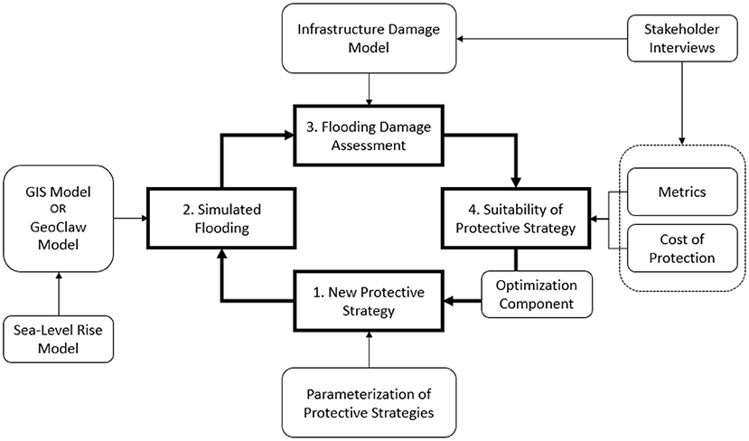
Figure 1. Conceptual layout of the proposed methodological framework (Miura et al., 2021c).

2.1. Parameterization of Protective Strategy

Each optimization iteration starts with the formulation of a new protective strategy based on the evaluation of the protective strategy in the previous iteration. For the first iteration loop, the comparison is made with the base case of no protective strategy at all. A protective strategy may consist of multiple protective measures implemented at different geographic (spatial) locations and at different times. For example, a protective strategy can consist of building a seawall with a 2 m height in 2020 and then adding an additional meter of height on top of it in 2050. In such a case, an appropriate discount rate has to be considered. Different variables can change for each protective strategy. For example, seawalls or elevating the coastline would need variables such as height, length, location, construction timing, etc. Based on these variables, the implementation cost can be computed. The cost estimate function should account for the local stakeholders' input as such costs may vary significantly locally according to Dols (2019). In the case of a seawall or elevated promenade along the coastline, the topographical data such as the digital elevation model (DEM) is modified by adding the designated wall height or the elevation height of the promenade onto the corresponding DEM cells at the locations where these protective measures are installed.

2.2. Flood Simulation

Two flood simulation models are employed in the optimization iterations: the GISSR model and the GEOCLAW model. The first iterations take advantage of the computational efficiency of the GISSR model to identify a rough estimate of the optimal solution. After that, the GEOCLAW model takes over to establish the optimal solution with high accuracy.

2.2.1. GIS-Based Subdivision-Redistribution Methodology (GISSR)

As the optimization process requires a large number of iterations, it is necessary to simulate storm-induced flooding with high computational efficiency. The GIS-based subdivision-redistribution methodology (GISSR) (Miura et al., 2021a) is extremely efficient computationally, but it is less accurate than the GEOCLAW model. This method is used to get a rough estimate of the optimal solution. The GISSR model requires topographical features (e.g., elevation, surface roughness, slope, etc.), time history data of the water level including surge, tide, and SLR, and a detailed description of the protective strategies as shown in Figure 2.

FIGURE 2

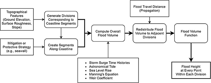
Figure 2. The GISSR flood simulation schematic diagram. Rectangles indicate inputs and rounded rectangles indicate processes.

At every point within the area under consideration, the flood height is computed using Manning's Equation and Weir's coefficient. The Manning's equation's coefficient is selected depending on the land type (e.g., urban, wetland) and surface roughness (e.g., the density of buildings) in the area of interest. If a scenario includes a seawall type of protective measure, Weir's coefficient is used to model a protective measure as a weir. The GISSR model first computes the overall flood volume during a hurricane event coming into the area under consideration by dividing the area into a number of smaller-scale “divisions.” This overall flood volume is redistributed to adjacent divisions accounting for water propagation. Once the flood volume in each division is established, it is translated into flood height within each division using a surface volume function (the flood height is uniform in a division).

The maximum surge height for a storm event is modeled by a modified beta distribution (Miura et al., 2021b). The corresponding frequency, duration, and time history are modeled using the method introduced in Lopeman et al. (2015). The simulation eventually establishes the flood height time history at every point within the area under consideration. The computed flood height at every point will be then used as input in the damage assessment model, as described in section 2.3. It should be noted that the GISSR model's accuracy has been validated with Hurricane Sandy's data, and the simulated inundated area and actual inundated area have been found to be almost identical (Miura et al., 2021a).

2.2.2. GeoClaw Model

During the last optimization iterations, flood simulations are carried out using GEOCLAW, a numerical solver for 2D shallow water equations over varying topographies as part of Clawpack (Conservation Laws Package) (Berger et al., 2011; Mandli et al., 2016; Clawpack Development Team, 2020). It is important to use this fluid-dynamics model in combination with the GISSR model since this provides a more physically accurate picture of how flood water will redistribute itself.

GEOCLAW takes as input a parameterized tropical cyclone (TC) and simulates the resulting storm surge by numerically solving the shallow water equations in the Atlantic basin with forcing terms from the TC. The TC is parameterized according to the model given by Holland (1980). For each time step, the TC has the following parameters: longitude and latitude of the eye of the storm, maximum wind speed, the radius at which maximum wind speed is attained, and central pressure. In the model of Holland (1980), these parameters allow a wind field to be reconstructed, which supplies the forcing terms to the shallow water equations.

For the simulations in this work, an ensemble of such parameterized TCs is run to calculate the expected peak storm surge height. The ensemble of storms is generated from the Columbia Hazard Model (CHAZ), a statistical-dynamical model due to Lee et al. (2018). The CHAZ model takes environmental parameters in a model of the Atlantic basin and stochastically generates TCs. The ensemble is comprised of those TCs that come close to NYC. GEOCLAW is also run on a parameterized model of Hurricane Sandy (National Hurricane Center, 2017) with different protective measure scenarios to examine their effectiveness. An example GEOCLAW run of Hurricane Sandy's track in the Atlantic Ocean and resulting storm surge on the US east coast is shown in Figure 3. A good predictive test of how efficient the protective strategy will be on potential future storms is obtained by carrying out a high-refinement shallow water simulation on storms derived from physical conditions.

FIGURE 3

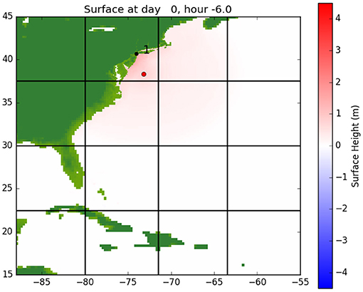
Figure 3. A plot at 6 h before landfall of a GEOCLAW simulation of Hurricane Sandy. The red dot indicates the eye of the storm and the black dot (1) indicates Battery Park in Lower Manhattan.

Each GEOCLAW storm-surge calculation is significantly more computationally expensive than the GISSR model. As a result, the entire space of protective strategies with GEOCLAW simulations is not searched. It is used to test the robustness of a small subset of GISSR suggested optimal solutions over different storms.

2.3. Damage Assessment

Using appropriate fragility functions (e.g., Hazus developed by Department of Homeland Security, Federal Emergency Management, 2018), the damage loss and economic loss for every component of the infrastructure can be quantified (including structural damage, damage to contents, and loss of use). The loss is computed for a given storm with known water height at any location within the geographical area considered (using the GISSR model or the GEOCLAW model). The losses are then added for all infrastructure components inside the geographical area considered to establish the overall loss from this specific event, and then for all of the events over the prescribed time frame.

2.3.1. Physical Damage and Economic Damage

For this study, the damage fragility curves provided by Hazus that was developed by the Department of Homeland Security, Federal Emergency Management (2018) are adopted with a slight modification for tall buildings that are prevalent in Lower Manhattan (Miura et al., 2021c). Damage functions are available for a variety of different classes of buildings, including various residential building types, commercial building types, utilities, factories, theaters, hospitals, nursing homes, churches, etc. The total damage/loss C_dmg to the built infrastructure in a target area related to physical loss is computed from the expression:

$\begin{array}{ll}{C}_{\text{dmg}}={\displaystyle \sum _i^{N_{\text{b}}}}{a}_i{D}_i(h_i)& (1)\end{array}$

where N_b is the total number of buildings/infrastructure components in the area, a_i is the total value/asset of building/infrastructure component i, and D_i is the percentage of the total replacement cost associated with flood height h_i observed at the location of building i. The flood height at each location h_i is computed by subtracting the critical elevation of each building from the total flood height computed in section 2.2.

Hazus has also developed functions to compute the economic losses due to suspended business operations during the restoration period. The losses taken into consideration in this article include income losses and inventory losses. If a building has commercial areas and did not collapse (buildings with over 50% damage are considered as collapsed), the damage functions for the total economic losses for each type can be computed as shown in Equations (2) and (3). The total economic losses are the total losses from all the buildings with commercial areas in the area under consideration.

Income loss:

$\begin{array}{ll}{C}_{\text{inc}}={\displaystyle \sum _i^{N_{\text{com}}}}(1-f_i)A_i(h_i)I_i{d}_i(h_i).& (2)\end{array}$

Inventory loss:

$\begin{array}{ll}{C}_{\text{inv}}={\displaystyle \sum _i^{N_{\text{inv}}}}{D}_i(h_i)A_i(h_i)G_i{B}_i.& (3)\end{array}$

where N_com is the total number of buildings with commercial areas, f_i is the income recapture factor for occupancy i, I_i is the income per day for occupancy i, and d_i is the loss of function time for the business in days. N_inv is the total number of commercial/industrial buildings dealing with inventories, A_i is the floor area at and below the flood height h_i, G_i denotes the annual gross sales for occupancy i, and B_i is the business inventory which is a percentage of gross annual sales. This applies to retail trade, wholesale trade, and industrial facilities. It should be noted that when a storm destroys more than 50% of a building, the building is considered as collapsed and will be demolished (not repaired) for any types of building/occupancy. It should be pointed out that no building collapsed in Lower Manhattan during Hurricane Sandy. Figure 4 shows the estimated damage percentage of each building in Lower Manhattan for the Hurricane Sandy scenario, and all the rates are lower than 50%. This result matches what happened in the city during this hurricane event (Miura et al., 2021c).

FIGURE 4

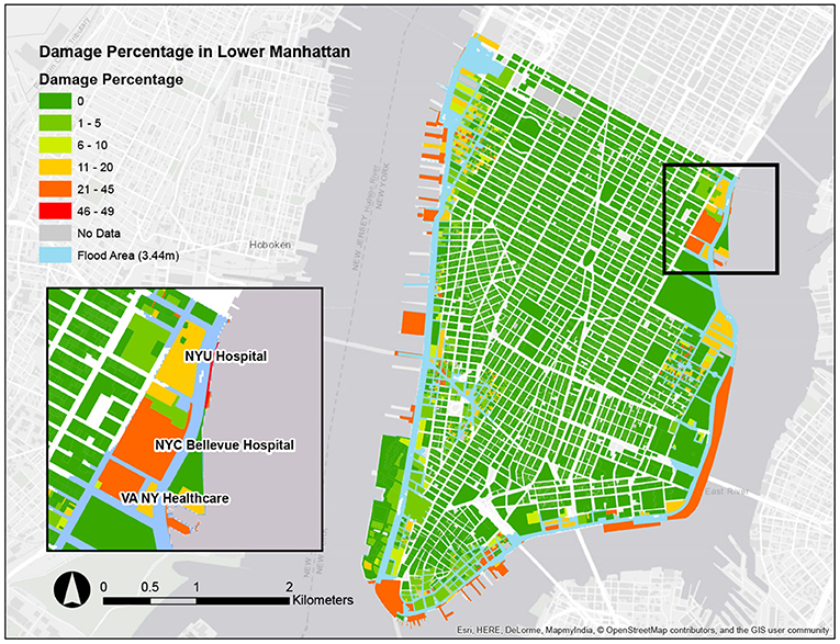
Figure 4. An example of damage percentage calculation for every building/infrastructure component during Hurricane Sandy in Lower Manhattan (Miura et al., 2021c).

The total direct damage cost is the summation of the total damage/loss C_dmg and the total economic losses (C_inc and C_inv). For the optimization iterations, the total direct damage cost is computed for all the randomly generated storm events during the prescribed time frame of interest with different batches of storms as inputs for each simulation. Figure 5 shows an example involving 1,000 simulations of cumulative damage assessment analysis over the next 80 years (2020–2100) in Lower Manhattan in NYC (without the presence of any protective measures). The storms in any year are separated into two seasons: warm season and cold season. The warm season is from June to November, and the cold season is from December to May. The storm characteristics in each season are physically different. For example, Hurricane Sandy is a warm-season storm, while a Nor'easter is a cold-season storm. The total accumulated damage costs in the year 2100 vary from $2 billion to $4 billion for cold season simulations, and from $1.5 to $9 billion for warm-season simulations, as every batch of storm surge events over the next 80 years is quite different because of the different randomly generated storm events. It should be noted that the storms in the warm season (depicted in red) are relatively less frequent but of larger magnitude. The storms in the cold season (depicted in blue) are vice versa. The different underlying physical mechanisms causing warm-season vs. cold-season storm events cause a larger scatter for warm-season cumulative damages compared to the corresponding cold-season cumulative damages, as can be seen in Figure 5. It is observed in Figure 5 that the damage costs of all the simulations start increasing nonlinearly from around the year 2070 because of the SLR effect.

FIGURE 5

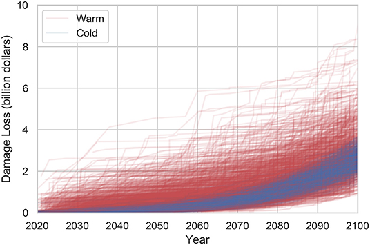
Figure 5. An example of the cumulative direct damage (i.e., the summation of physical damage loss, income loss, inventory loss, and loss from interdependencies) from storm-induced flooding over the next 80 years (2020–2100) resulting from 1,000 different simulations in Lower Manhattan in NYC (without any protective measures present). The total cumulative damage cost/loss over the years varies for each simulation because of the different randomly generated storm events in each one of the 1,000 simulations. Blue lines indicate damage losses from cold-season storms. Red lines indicate damage losses from warm-season storms.

2.3.2. Economic Damage due to Inoperability and Interconnectivity

When an infrastructure component is inoperable due to flooding, the interdependency (interconnectivity) of infrastructure components (infrastructures) may trigger additional financial impacts on other sectors of the infrastructure. This extra economic impact should be accounted for in the damage assessment. During Hurricane Sandy in 2012, there was a major power outage in Lower Manhattan due to an explosion at a flooded utility facility on the Lower East Side. This accident caused not only millions of people to be without electricity, but other infrastructure sectors such as hospitals, fuel distributors, businesses, and many more, to be partially or fully non-functional. Using the Inoperability Input-Output Model (IIM) (Haimes and Jiang, 2001) based on the I-O model introduced originally by Leontief (1986) and the damage cost computed using the modified Hazus model as described in section 2.3.1, economic loss due to interdependencies of the infrastructures can be calculated using the inoperability ratio. This inoperability ratio is highly dependent on the region of interest as it indicates how much each sector depends on each other financially. For example, a highly urbanized area such as NYC may have higher impacts on industries such as business and commerce.

For NYC, Cimellaro et al. (2019) evaluated Hurricane Sandy induced damages and established the inoperability ratios for the metropolitan area based on IIM. Using the inoperability ratio matrix, this study quantified the losses due to the inoperability of utilities and transportation infrastructures.

2.4. Stakeholders' Feedback Input

A set of interviews with city and state stakeholders who have first-hand knowledge of the NYC area's infrastructures have been planned to check the suitability/acceptability of the optimization model (including flood estimate models, damage assessment models, and information on interdependencies of the infrastructures in the city) and of its results concerning the optimal protective strategy. The first interviews were conducted in the early stages of the project. The stakeholders provided feedback on the models and provided information on the interdependencies of the infrastructures in the target area. The second set of interviews was conducted after reflecting on the first set's inputs, in order to further refine the method and its results. Based on the outcomes of these interviews, the optimization model, including flood simulation models and damage assessment models, will be updated so that the model can generate socially acceptable optimal solutions.

2.5. Optimization

The methodology optimizes coastal protective strategies (this can be a combination of multiple protective measures) given a constraint, here the overall budget for building protection and mitigation measures. For a prescribed budget and a prescribed time horizon of N years (N can be 20, 50, 100 years, or any other number), the optimal solution is the one that minimizes the sum of the total storm-induced losses plus the cost of implementing the protective strategy. The budget can be defined arbitrarily by the user, and different budget levels can be considered to explore different corresponding optimal solutions.

The first step is to calculate the overall expected losses over the N years from all randomly generated storms during this period, without any protective strategy implemented. These losses are denoted by L_no (losses are considered in a statistical sense in this section as L_no is a random variable computed/realized M times from M different simulations over the period of N years).

Each selected protective strategy at a given iteration of the optimization process is examined using the same set of M simulations of randomly generated storms over N years that was considered for the base case of “no protective strategy/measures.” For a selected protective strategy, its total cost (total implementation cost L_co of the strategy plus overall losses L_ps from all the storms during the period of N years) is computed, again in a statistical sense. This total cost has to be less than L_no for the protective strategy to be preferable to the base case of “no protective strategy implemented”:

$\begin{array}{ll}{L}_{\text{co}}+L_{\text{ps}}<L_{\text{no}}.& (4)\end{array}$

If Equation (4) is not satisfied for a specific protective strategy, then this strategy is unacceptable (since the case of no protective strategy has a lower overall cost).

The total cost is estimated using the damage assessment models (section 2.3) with the estimated flood heights [the outcome of the GISSR model (section 2.2.1) and the GEOCLAW model (section 2.2.2)]. As described previously, the GISSR model is used to find a rough estimate of the optimal solution, and the GEOCLAW model fine-tunes this rough estimate of the optimal solution. Since the frequency of storms and their magnitude are uncertain over the prescribed period, the methodology uses multiple simulations M over the prescribed N years to find a histogram and a corresponding expected value and standard deviation of the total cost. Each simulation uses a different set of randomly generated storms modeled over the N years.

For a preliminary demonstration of the methodology, this paper uses a brute-force iterative approach for the optimization on a discrete set of protective measures. Each brute-force optimization loop returns a different histogram/probability distribution of the total cost over the N years. If the summation of the implementation cost and overall losses of the protective strategy at iteration (p) is less than that of iteration (p − 1), then the protective strategy at iteration (p) becomes the temporary optimum solution. Otherwise, the protective strategy at iteration (p − 1) remains the temporary optimal solution, and a new protective strategy is tested against it. This procedure is expressed as follows:

If (L_co + L_ps)_(p−1) > (L_co + L_ps)_(p), then (L_co + L_ps)_(p) becomes the new temporary optimal strategy and a new protective strategy is tested against it. (5a)

If (L_co + L_ps)_(p−1) < (L_co + L_ps)_(p), then (L_co + L_ps)_(p−1) remains as the temporary optimal strategy, (L_co + L_ps)_(p) is discarded, and a new protective strategy is tested against (L_co + L_ps)_(p−1). (5b)

The iterations continue until (L_co + L_ps) stabilizes, without any substantial further reduction possible in subsequent iterations. It is reminded that as with L_no, L_ps is considered in a statistical sense.

The optimization variables can change depending on the protective measures considered. For example, in the case of seawalls as protective measures, the variables would be location, height, length, and construction timing.

3. Coastal Protection Optimization in New York City

Lower Manhattan in NYC is selected as a testbed because of the city's complex infrastructure and data availability. As this is the first application of the methodology, the protective measure considered is only a seawall (as there are planned projects called the Big U (Rebuild By Design, 2015) and the East Side Coastal Resiliency Project (City of New York, 2021) involving a seawall in Lower Manhattan).

The optimal solution is narrowed down using the GISSR model (Miura et al., 2021a) and then is validated with the GEOCLAW model (Berger et al., 2011). Although the GEOCLAW model is in general used to fine-tune the optimal solution established by GISSR, here, it is only used to validate it.

3.1. Future Anticipated Storms and Sea Level Rise

Surge data for storms are generated using the methodology introduced by Lopeman et al. (2015) and a modified beta distribution to model the maximum surge height of a storm. This study accounts for SLR at the Battery, NY, as predicted by Horton et al. (2015) and Gornitz et al. (2019). The projected SLR values are shown in Table 1. The projections are estimated with the 2000–2004 period as the reference baseline. For each year examined, the average of the 25th and 75th percentile estimates from Table 1 is used in this study (which is referred to as the middle estimate). Hence, the middle SLR estimates employed for the 2050s, 2080s, and 2100 are 0.406, 0.724, and 0.9145 m, respectively.

TABLE 1

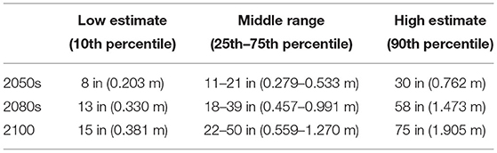
Table 1. New York City sea level rise projections (the 2000–2004 period is considered as the sea level baseline (Horton et al., 2015; Gornitz et al., 2019).

As the number of storms and the corresponding maximum storm surge values are uncertain, M simulations are performed over the N years considered. Each simulation has a different number and magnitude of storms, and these are modeled as random variables. The peak storm surge height is modeled with a modified beta distribution (Miura et al., 2021b). The number of simulations M is set equal to 1,000, and the prescribed number of years N is set equal to 80 (from 2020 to 2100) for this study. Figure 6 depicts the peak water levels (peak storm surge + SLR + tidal height) for storms randomly generated over the 80-year period from 2020 to 2100, accounting for a middle estimate of SLR. Figure 6 displays the randomly generated storms from one simulation among the M = 1, 000 considered. The storms in the warm season (depicted as red dots) are relatively less frequent but larger in magnitude on the average. The storms in the cold season (depicted as blue dots) are the other way around. Figure 7 displays all the storms from all the M = 1, 000 simulations considered. Even moderate storms close to the end of this 80-year period can become severe ones in overall water height because of SLR.

FIGURE 6

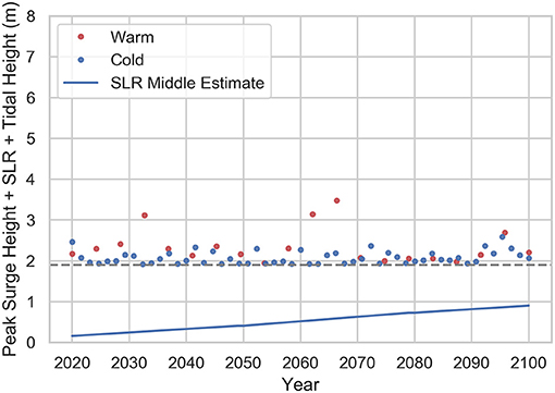
Figure 6. An example of one simulation of randomly generated storms expressed through their corresponding peak water levels (peak storm surge + SLR + tidal height) over the 80-year period considered (2020–2100). The blue dots depict peak storm surges in cold season. The red dots depict peak storm surges in warm season. Middle SLR estimate (Horton et al., 2015; Gornitz et al., 2019) is considered. SLR is denoted by the continuous sloped blue line. The dashed horizontal gray line indicates the 1.9 m threshold, below which there is no flooding observed in Lower Manhattan.

FIGURE 7

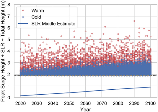
Figure 7. One thousand simulations of randomly generated storms expressed through their corresponding peak water levels (peak storm surge + SLR + tidal height) over the 80-year period considered (2020–2100). The blue dots depict peak storm surges in cold season. The red dots depict peak storm surges in warm season. Middle SLR estimate (Horton et al., 2015; Gornitz et al., 2019) is considered. SLR is denoted by the continuous sloped blue line. The dashed horizontal gray line indicates the 1.9 m threshold, below which there is no flooding observed in Lower Manhattan.

3.2. Potential Protective Measures

Although coastal protective measures can be numerous as mentioned earlier, this article considers only a seawall in Lower Manhattan for demonstration purposes. The seawall configuration is optimized using multiple variables, including its height, length, and specific location as indicated in Figure 8.

FIGURE 8

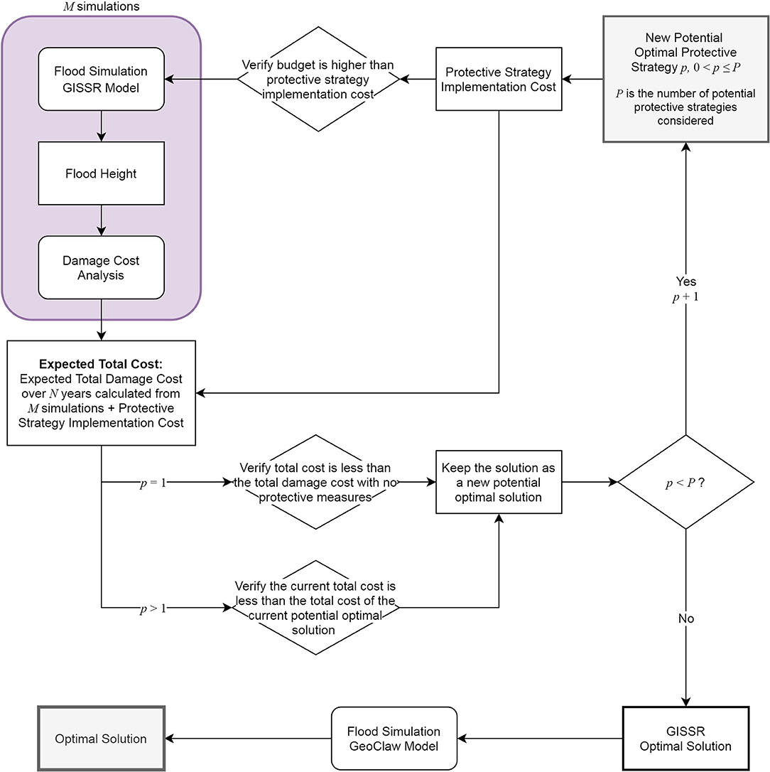
Figure 8. Coastal protection optimization flow chart for the preliminary study considered in this paper. Rectangles indicate inputs and rounded rectangles indicate processes.

Based on studies of cost estimates for flood adaptation/mitigation including seawalls (Aerts et al., 2013; Aerts, 2018) and the NY and NJ harbor and tributaries focus area feasibility study (HATS) (Dols, 2019), the construction cost estimate of a seawall in this study is modeled as shown below:

$\begin{array}{ll}{L}_{{\text{co}}_{\text{wall}}}=\$49,212h_{\text{wall}}{l}_{\text{wall}}& (6)\end{array}$

where, L_cowall is the seawall's construction cost in US dollars, h_wall is the seawall height in meters, and l_wall is the seawall length in meters. In most of its length around Lower Manhattan, the currently considered Big U project is designed as an elevated promenade instead of just a seawall or floodwall. The construction cost of such an elevated promenade is estimated by Dols (2019).

The $49,212 cost value in Equation (6) corresponds to a wall segment having a length equal to one meter and height also equal to one meter.

3.3. Optimal Solution

The optimal solution in this study is the protective seawall/elevated promenade configuration that minimizes the total expected cost given a prescribed budget. The total expected cost includes the total damage cost (Equations 1–3) and the implementation/building cost of the protective seawall given in Equation (6) (in the following, the elevated promenade/seawall is simply going to be referred as seawall). The damage costs are computed using the dataset provided by the New York City Department of City Planning (2018) for each individual building with property assets data.

The minimum expected cost is found by an exhaustive brute-force search using a discretized set of the protective measure variables (h_wall, i_wall0, i_wallf).

3.3.1. Objective Function and Constraints

The objective function of the optimization problem is defined as:

$\begin{array}{ll}{\displaystyle \underset{\text{x}}{min}}\left\{L_{\text{co}}(\text{x})+{𝔼}_S\left[{\displaystyle \sum _{s\in S_j}}f(\text{x};s)\right]\right\}& (7)\end{array}$

where f(x; s) is the total damage cost (physical damage and economic loss) from each storm event s, S_j is one set of randomly generated storms to hit NYC in the period 2020–2100 considered here, 𝔼_S is the expected value over all M = 1, 000 simulations considered, and L_co is the total implementation/building cost of the protective strategy. The decision variable is:

$\begin{array}{ll}\text{x}=(h_{\text{wall}},i_{{\text{wall}}_0},i_{{\text{wall}}_f})& (8)\end{array}$

where, i_wall0 and i_wallf represent the start and end locations of the seawall, respectively. The constraints are:

$\begin{array}{l}0\le h_{\text{wall}}\le 5\text{m}\\ 0\le i_{{\text{wall}}_0}\le i_{{\text{wall}}_f}\le i_{{\text{wall}}_F}\\ L_{\text{co}}\le L_{\text{budget}}& (9)\end{array}$

As described in Equation (4), the total cost (the summation of the implementation cost L_co and overall losses L_ps), must be less than the overall losses without any protective measures L_no. This is ensured by including the no seawall scenario in the search domain. L_budget is the prescribed budget.

In the implementation, an exhaustive search is performed to determine the aforementioned minimum total expected cost over a discretized set of seawalls, specifically h_wall ∈ {0.5, 1.0, 1.5, …, 5.0} measured in meters, and i_wall0, i_wallf ∈ {0, 1, 2, …, 162} corresponding to 163 locations along the coastline of Lower Manhattan, spaced 100 meters apart. Consequently, the seawall length can be computed:

$\begin{array}{ll}{l}_{\text{wall}}=100\text{m}(i_{{\text{wall}}_f}-i_{{\text{wall}}_0})& (10)\end{array}$

1,000 sets of randomly generated storms to hit NYC in the period 2020–2100 are simulated (M = 1, 000 simulations: ${\left\{S_j\right\}}_{j=1}^{1,000}$). Consequently, the objective function in Equation (7) can be rewritten as:

$\begin{array}{ll}{L}_{\text{co}}(\text{x})+\frac{1}{1,000}{\displaystyle \sum _{j=1}^{1,000}}{\displaystyle \sum _{s\in S_j}}f(\text{x};s)& (11)\end{array}$

3.3.2. Optimal Solution Using the GISSR model

The optimal solution minimizing the total expected cost (Equations 7, 11) differs significantly as a function of the level of the prescribed budget. Figure 9 plots the total expected cost of the optimal solution as a function of the prescribed budget (as the total cost is a random variable, its expected value is used here). With zero budget available (no protective measures), the expected value of the total damage cost is around $5 billion. As the level of the prescribed budget increases, the total expected damage cost decreases, as well as the total expected cost. At the $1.7 billion budget level, the total expected cost stabilizes at around $2.4 billion. Further increases of the prescribed budget up to $2.4 billion do not produce any significant variation in the $2.4 billion value of the total expected cost. When the budget becomes larger than $2.4 billion, the total expected cost starts increasing again as seen in Figure 9. It should be noted that it is possible to reduce the expected damage cost to zero, but the necessary budget is relatively high (a budget of around $4 billion is necessary to achieve the zero expected damage cost).

FIGURE 9

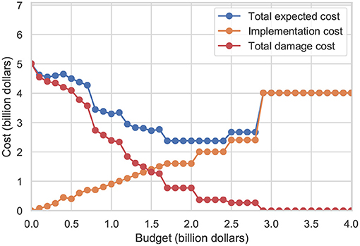
Figure 9. The total expected cost of an optimal solution as a function of the prescribed budget for the Lower Manhattan area. Orange dots represent the implementation cost of the optimal protective strategy, red dots represent the corresponding total damage cost, and blue dots represent the sum of the orange and red dots (total expected cost). The total expected cost of the optimal solution (blue dots) varies significantly as a function of the prescribed budget.

Figure 10 displays the actual optimal protective seawall measures for four different levels of the prescribed budget. It is clear that different budget levels lead to different optimal seawall solutions. The $0.5, $1.0, and $1.5 billion budgets produce optimal solutions with seawalls over only a part of the entire coastline. The $2.1 billion budget yields an optimal solution with a 2.5 m high seawall over the entire length of the coastline of Lower Manhattan.

FIGURE 10

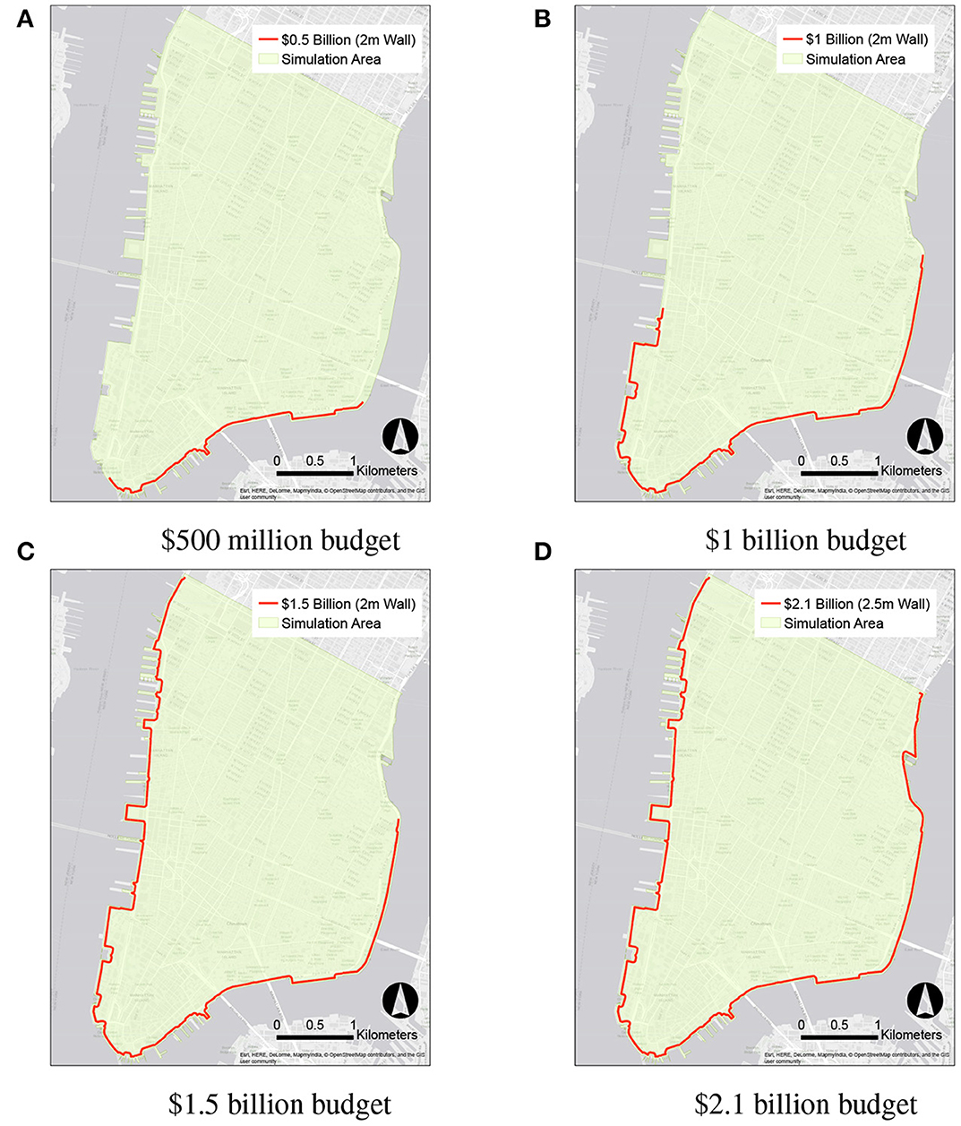
Figure 10. Optimal protective seawall measures corresponding to four different prescribed budget levels. (A) $500 million budget, (B) $1 billion budget, (C) $1.5 billion budget, (D) $2.1 billion budget.

3.3.3. Flood Simulations Using the GeoClaw Model

In order to validate and verify the robustness of the optimal solutions found using GISSR, tests are performed against a number of storms modeled in GEOCLAW. A representative point at (−74.013, 40.705) is selected in Lower Manhattan, and the peak flood height at this point is calculated using GEOCLAW with different storms and different protective seawalls in front of it.

Figure 11 shows results of Hurricane Sandy simulations with different seawalls and no SLR. The images show the flood height and sea surface height at the time of peak flood height. The $1 billion seawall is in front of our point of interest, but because of the high storm surge, water can get over the seawall and around the sides of the wall (see Figures 10B, 11C). As a result, much of Lower Manhattan is inundated, even areas directly behind the wall. The $2.1 billion wall shows some inundation, though much less (see Figures 10D, 11D).

FIGURE 11

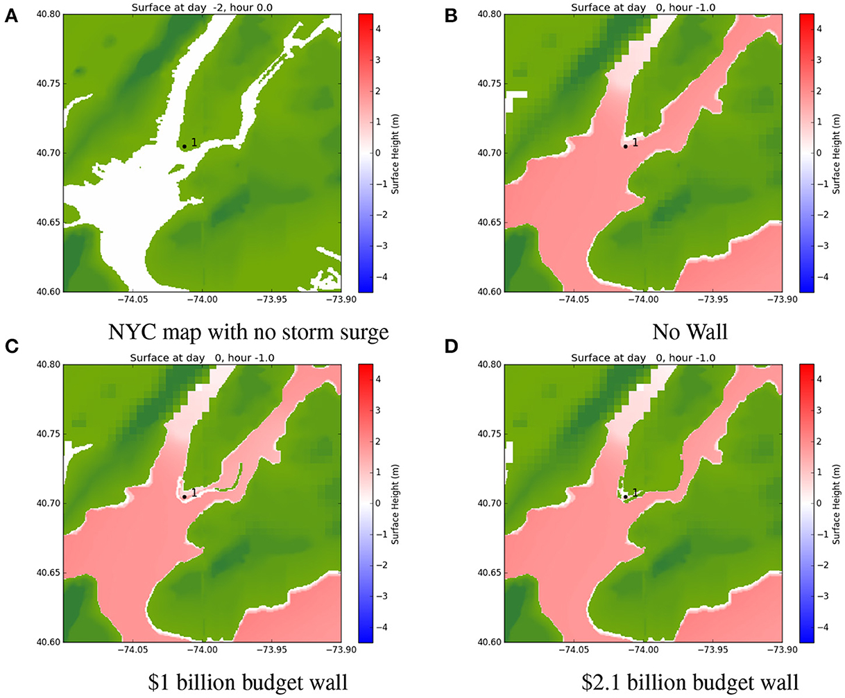
Figure 11. Selected point in Lower Manhattan (denoted by 1) where peak flood heights are calculated for Hurricane Sandy and various different seawalls, using GEOCLAW. (A) NYC map with no storm surge, (B) no wall, (C) $1 billion budget wall, (D) $2.1 billion budget wall.

GEOCLAW runs of Hurricane Sandy were also performed with SLR corresponding to the middle estimate for the 2020–2100 period. Figure 12 shows the corresponding peak flood heights at the selected point of interest. Figure 12 indicates that for Sandy without SLR, the flood protection offered by the 1 billion wall is little to nothing at the selected point of interest, whereas the $2.1 billion wall provides greater protection. With SLR, especially from the year 2080 and onwards, both walls begin to become obsolete, showing only minimal levels of protection.

FIGURE 12

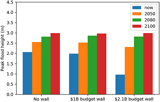
Figure 12. A comparison of peak flood heights at the selected point in Lower Manhattan (identified by 1 in Figure 11) for different optimal protective measures and different levels of SLR.

GEOCLAW simulations were also run using an ensemble of 26 TCs that reach land near the NYC area selected from the synthetically generated storms in the Atlantic Ocean in a model of the current climate with no SLR. The mean peak flood heights of the ensemble of 26 storms at the same point of interest depicted in Figure 11 are plotted in Figure 13. The results show that the $1 billion wall provides some protection in comparison to the no wall situation. This difference happens because the storm ensemble contains a number of storms with different induced storm surges, including smaller ones that do not overtop the wall. The $2.1 billion wall provides only a marginal further reduction in the mean peak flood height.

FIGURE 13

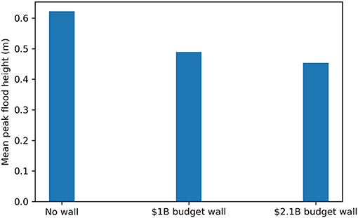
Figure 13. Mean peak flood heights at the point depicted in Figure 11 resulting from the selected ensemble of 26 TCs.

3.3.4. Comparison of the GISSR Model and the GeoClaw Model

The GEOCLAW model is used in section 3.3.3 to validate the protective capability of GISSR-established optimal solutions against Hurricane Sandy and other possible TCs over the 2020–2100 period. As Figure 12 shows, both walls examined show little protection past 2050, and the $1 billion wall shows little protection even at present against Hurricane Sandy. Against the ensemble of TCs, both walls show some protective capability compared to no wall. This is because the ensemble of storms had on average lower intensity than Hurricane Sandy. The storm inputs to the GEOCLAW simulations in this study are all TCs categorized as warm-season storms and are therefore relatively more intense than cold-season storms. For the most intense storms, the walls lose their protectiveness altogether as the flooding completely overtops them and inundates the area behind them. On the other hand, the GISSR model accounts for both cold and warm season storms. This explains why in the GISSR model, the $2.1 billion wall provides significantly more protection than the $1 billion wall, which in turn provides significantly more protection than no wall at all, even into the year 2100. Together these models show that a large advantage of the walls is their protective capability against frequent smaller storms. When faced with multiple superstorms such as Sandy and SLR, the two different examined seawalls start to diminish in their effectiveness.

4. Conclusion and Discussion

This study provides preliminary results for the optimal protective measures for Lower Manhattan in NYC, given a prescribed budget. The optimal solution is determined to minimize the expected total cost from all the potential storms over the 80-year period from 2020 to 2100, given a prescribed budget. The methodology combines hydrology and physics components, socio-economic factors, and stakeholder feedback to properly model the complex interdependency of the infrastructures. A discrete and exhaustive set of seawalls with different heights, lengths, and locations is examined in this study, and the corresponding expected total costs (i.e., damage cost and implementation/building cost) are computed. The optimal solution varies widely depending on the budget, which can be defined arbitrarily by users. A seawall with a height of 2.5 m along the entire coastline of Lower Manhattan with a budget of $2.1 billion appears to prevent major flooding sufficiently well, as the expected damage cost is decreased significantly. An optimal solution does not necessarily reduce the damage cost to zero since making the damage cost zero would significantly increase the implementation/building cost. The GEOCLAW model showed that this seawall might become obsolete past 2050 against an ensemble of major TC storms like Hurricane Sandy and SLR. However, this methodology can help decision-makers evaluate future risks and make optimal decisions.

The results and conclusions provided in this work demonstrate the capability of the proposed methodology in optimizing coastal protective measures given a prescribed budget. This study's main contribution is to introduce the methodology and demonstrate the nature of the results/conclusions. If different SLR projections are used instead of the selected ones in this study (i.e., Horton et al., 2015; Gornitz et al., 2019), the corresponding results and conclusions are expected to be different.

Only the height, length, and location of seawalls were taken into account for this study for the sake of simplicity in demonstrating the capabilities of the methodology. In the future, it is suggested to include other variables such as construction timing, other measures (e.g., structural, nature-based, financial, and political), or a combination of thereof to determine a comprehensive optimal strategy for a target region.

A brute-force optimization approach was employed for simplicity in this study. More sophisticated optimization algorithms should eventually be employed to speed up the search for the optimal solution, such as a derivative-free descent algorithm on the protective measure parameters or a stochastic descent approach.

Data Availability Statement

This study uses the dataset and tool as listed: Berger et al. (2011), Mandli et al. (2016), National Hurricane Center (2017), Department of Information Technology & Telecommunications (2018), New York City Department of City Planning (2018), Clawpack Development Team (2020), Miura (2020).

Author Contributions

YM, PD, KM, and GD contributed to conception and design of the study. YM, PD, and KM organized the database. YM and PD performed the analysis. YM wrote the first draft of the manuscript. PD wrote sections of the manuscript. All authors contributed to manuscript revision, read, and approved the submitted version.

Conflict of Interest

The authors declare that the research was conducted in the absence of any commercial or financial relationships that could be construed as a potential conflict of interest.

Publisher's Note

All claims expressed in this article are solely those of the authors and do not necessarily represent those of their affiliated organizations, or those of the publisher, the editors and the reviewers. Any product that may be evaluated in this article, or claim that may be made by its manufacturer, is not guaranteed or endorsed by the publisher.

Acknowledgments

The authors gratefully acknowledge support by the National Science Foundation under Grants No. DMS-1720288 and OAC-1735609.

References

Abadie, L. M., Jackson, L. P., de Murieta, E. S., Jevrejeva, S., and Galarraga, I. (2020). Comparing urban coastal flood risk in 136 cities under two alternative sea-level projections: RCP 8.5 and an expert opinion-based high-end scenario. Ocean Coast. Manage. 193:105249. doi: 10.1016/j.ocecoaman.2020.105249

CrossRef Full Text | Google Scholar

Adger, W. N., Arnell, N. W., and Tompkins, E. L. (2005). Successful adaptation to climate change across scales. Global Environ. Change 15, 77–86. doi: 10.1016/j.gloenvcha.2004.12.005

CrossRef Full Text | Google Scholar

Aerts, J. C. (2018). A review of cost estimates for flood adaptation. Water 10:1646. doi: 10.3390/w10111646

CrossRef Full Text

Aerts, J. C., Botzen, W. W., de Moel, H., and Bowman, M. (2013). Cost estimates for flood resilience and protection strategies in New York city. Ann. N. Y. Acad. Sci. 1294, 1–104. doi: 10.1111/nyas.12200

PubMed Abstract | CrossRef Full Text | Google Scholar

Berger, M. J., George, D. L., LeVeque, R. J., and Mandli, K. T. (2011). The GeoClaw software for depth-averaged flows with adaptive refinement. Adv. Water Res. 34, 1195–1206. doi: 10.1016/j.advwatres.2011.02.016

CrossRef Full Text | Google Scholar

Burkett, V. R., Zilkoski, D. B., and Hart, D. A. (2002). “Sea-level rise and subsidence: implications for flooding in New Orleans, Louisiana,” in US Geological Survey Subsidence Interest Group Conference (Galveston, TX: US Geological Survey), 63–71.

Google Scholar

Cimellaro, G. P., Crupi, P., Kim, H. U., and Agrawal, A. (2019). Modeling interdependencies of critical infrastructures after hurricane sandy. Int. J. Disast. Risk Reduct. 38:101191. doi: 10.1016/j.ijdrr.2019.101191

CrossRef Full Text | Google Scholar

City of New York (2021). The East Side Coastal Resiliency Project. City of New York.

Clawpack Development Team (2020). Clawpack Software. Version 5.7.1. Clawpack Development Team.

Department of Homeland Security, Federal Emergency Management Agency (2018). Hazus. Department of Homeland Security, Federal Emergency Management Agency.

Department of Information Technology & Telecommunications (2018). Building Footprints. Department of Information Technology & Telecommunications.

Dols, C. (2019). New York–New Jersey Harbor and Tributaries Coastal Storm Risk Management Feasibility Study Interim Report Cost Appendix. US Army Corps of Engineers.

Dupuits, E., Schweckendiek, T., and Kok, M. (2017). Economic optimization of coastal flood defense systems. Reliabil. Eng. Syst. Saf. 159, 143–152. doi: 10.1016/j.ress.2016.10.027

CrossRef Full Text | Google Scholar

Gornitz, V., Oppenheimer, M., Kopp, R., Horton, R., Orton, P., Rosenzweig, C., et al. (2020). Enhancing New York city's resilience to sea level rise and increased coastal flooding. Urban Clim. 33:100654. doi: 10.1016/j.uclim.2020.100654

CrossRef Full Text | Google Scholar

Gornitz, V., Oppenheimer, M., Kopp, R., Orton, P., Buchanan, M., Lin, N., et al. (2019). New York city panel on climate change 2019 report chapter 3: Sea level rise. Ann. N. Y. Acad. Sci. 1439, 71–94. doi: 10.1111/nyas.14006

PubMed Abstract | CrossRef Full Text | Google Scholar

Haimes, Y. Y., and Jiang, P. (2001). Leontief-based model of risk in complex interconnected infrastructures. J. Infrastruct. Syst. 7, 1–12. doi: 10.1061/(ASCE)1076-0342(2001)7:1(1)

CrossRef Full Text | Google Scholar

Hirabayashi, Y., Mahendran, R., Koirala, S., Konoshima, L., Yamazaki, D., Watanabe, S., et al. (2013). Global flood risk under climate change. Nat. Clim. Change 3, 816–821. doi: 10.1038/nclimate1911

PubMed Abstract | CrossRef Full Text | Google Scholar

Holland, G. J. (1980). An analytic model of the wind and pressure profiles in hurricanes. Month. Weath. Rev. 108, 1212–1218. doi: 10.1175/1520-0493(1980)108<1212:AAMOTW>2.0.CO;2

CrossRef Full Text | Google Scholar

Horton, R., Little, C., Gornitz, V., Bader, D., and Oppenheimer, M. (2015). New York city panel on climate change 2015 report chapter 2: Sea level rise and coastal storms. Ann. N. Y. Acad. Sci. 1336, 36–44. doi: 10.1111/nyas.12593

PubMed Abstract | CrossRef Full Text | Google Scholar

Jonkman, S., Brinkhuis-Jak, M., and Kok, M. (2004). Cost benefit analysis and flood damage mitigation in the Netherlands. Heron 49, 95–111. http://heronjournal.nl/49-1/5.pdf

Google Scholar

Lee, C.-Y., Tippett, M. K., Sobel, A. H., and Camargo, S. J. (2018). An environmentally forced tropical cyclone hazard model. J. Adv. Model. Earth Syst. 10, 223–241. doi: 10.1002/2017MS001186

CrossRef Full Text | Google Scholar

Leontief, W. (1986). Input-Output Economics. Oxford: Oxford University Press. doi: 10.1057/978-1-349-95121-5_1072-1

CrossRef Full Text | Google Scholar

Lin, N., Emanuel, K., Oppenheimer, M., and Vanmarcke, E. (2012). Physically based assessment of hurricane surge threat under climate change. Nat. Clim. Change 2, 462–467. doi: 10.1038/nclimate1389

CrossRef Full Text | Google Scholar

Longenecker, H. E., Graeden, E., Kluskiewicz, D., Zuzak, C., Rozelle, J., and Aziz, A. L. (2020). A rapid flood risk assessment method for response operations and nonsubject-matter-expert community planning. J. Flood Risk Manage. 13:e12579. doi: 10.1111/jfr3.12579

CrossRef Full Text | Google Scholar

Lopeman, M., Deodatis, G., and Franco, G. (2015). Extreme storm surge hazard estimation in lower manhattan. Nat. Hazards 78, 355–391. doi: 10.1007/s11069-015-1718-6

CrossRef Full Text | Google Scholar

Mandli, K. T., Ahmadia, A. J., Berger, M., Calhoun, D., George, D. L., Hadjimichael, Y., et al. (2016). Clawpack: building an open source ecosystem for solving hyperbolic PDES. PeerJ Comput. Sci. 2:e68. doi: 10.7717/peerj-cs.68

CrossRef Full Text | Google Scholar

Marcos, M., Calafat, F. M., Berihuete, Á., and Dangendorf, S. (2015). Long-term variations in global sea level extremes. J. Geophys. Res. 120, 8115–8134. doi: 10.1002/2015JC011173

CrossRef Full Text | Google Scholar

Marcos, M., and Woodworth, P. L. (2017). Spatiotemporal changes in extreme sea levels along the coasts of the North Atlantic and the Gulf of Mexico. J. Geophys. Res. 122, 7031–7048. doi: 10.1002/2017JC013065

CrossRef Full Text | Google Scholar

Marsooli, R., Lin, N., Emanuel, K., and Feng, K. (2019). Climate change exacerbates hurricane flood hazards along us Atlantic and gulf coasts in spatially varying patterns. Nat. Commun. 10, 1–9. doi: 10.1038/s41467-019-11755-z

PubMed Abstract | CrossRef Full Text | Google Scholar

Miura, Y. (2020). High-Speed Gis Flood Simulation. Available online at: https://github.com/ym2540/GIS_FloodSimulation

Miura, Y., Mandli, K. T., and Deodatis, G. (2021a). High-speed gis-based simulation of storm surge-induced flooding accounting for sea level rise. Nat. Hazards Rev. 22:04021018. doi: 10.1061/(ASCE)NH.1527-6996.0000465

CrossRef Full Text | Google Scholar

Miura, Y., Mandli, K. T., and Deodatis, G. (2021b). Storm surge modeling with modified beta distributions. In Preparation.

Google Scholar

Miura, Y., Qureshi, H., Ryoo, C., Dinenis, P. C., Li, J., Mandli, K. T., et al. (2021c). A methodological framework for determining an optimal coastal protection strategy against storm surges and sea level rise. Nat. Hazards 107, 1821–1843. doi: 10.1007/s11069-021-04661-5

CrossRef Full Text | Google Scholar

National Hurricane Center (2017). Automated Tropical Cyclone Forecast (ATCF) Data Files/Text Files. National Hurricane Center. Available online at: https://ftp.nhc.noaa.gov/atcf

New York City Department of City Planning (2018). Mappluto. New York City, NY: Department of City Planning (accessed August 15, 2020).

Parris, A. S., Bromirski, P., Burkett, V., Cayan, D. R., Culver, M. E., Hall, J., et al. (2012). Global Sea Level Rise Scenarios for the United States National Climate Assessment. NOAA technical report, OAR CPO.

Rebuild By Design (2015). The Big U. Online, New York. (accessed August 15, 2020).

Reguero, B. G., Beck, M. W., Bresch, D. N., Calil, J., and Meliane, I. (2018). Comparing the cost effectiveness of nature-based and coastal adaptation: a case study from the gulf coast of the United States. PLoS ONE 13:e0192132. doi: 10.1371/journal.pone.0192132

PubMed Abstract | CrossRef Full Text | Google Scholar

Stocker, T. F., Qin, D., Plattner, G.-K., Tignor, M., Allen, S. K., Boschung, J., et al. (2013). Climate Change 2013: The Physical Science Basis. Contribution of working group I to the fifth assessment report of the intergovernmental panel on climate change, New York: Cambridge University Press, 1535.

Google Scholar

Sweet, W. V. (2014). Sea Level Rise and Nuisance Flood Frequency Changes Around the United States. US Department of Commerce, National Oceanic and Atmospheric Administration.

Google Scholar

Taherkhani, M., Vitousek, S., Barnard, P. L., Frazer, N., Anderson, T. R., and Fletcher, C. H. (2020). Sea-level rise exponentially increases coastal flood frequency. Sci. Rep. 10, 1–17. doi: 10.1038/s41598-020-62188-4

PubMed Abstract | CrossRef Full Text | Google Scholar

Ward, P. J., Jongman, B., Aerts, J. C., Bates, P. D., Botzen, W. J., Loaiza, A. D., et al. (2017). A global framework for future costs and benefits of river-flood protection in urban areas. Nat. Clim. Change 7, 642–646. doi: 10.1038/nclimate3350

CrossRef Full Text | Google Scholar

Ward, P. J., Jongman, B., Salamon, P., Simpson, A., Bates, P., De Groeve, T., et al. (2015). Usefulness and limitations of global flood risk models. Nat. Clim. Change 5, 712–715. doi: 10.1038/nclimate2742

CrossRef Full Text | Google Scholar

Winsemius, H., Van Beek, L., Jongman, B., Ward, P., and Bouwman, A. (2013). A framework for global river flood risk assessments. Hydrol. Earth Syst. Sci. 17, 1871–1892. doi: 10.5194/hess-17-1871-2013

CrossRef Full Text | Google Scholar

Zwaneveld, P. J., and Verweij, G. (2014). Safe Dike Heights at Minimal Costs. The Hague.

Google Scholar