Hurricane Scenario Generation for Uncertainty Modeling of Coastal and Inland Flooding

Hurricanes often induce catastrophic flooding due to both storm surge near the coast, and pluvial and fluvial flooding further inland. In an effort to contribute to uncertainty quantification of impending flood events, we propose a probabilistic scenario generation scheme for hurricane flooding using state-of-art hydrological models to forecast both inland and coastal flooding. The hurricane scenario generation scheme incorporates locational uncertainty in hurricane landfall locations. For an impending hurricane, we develop a method to generate multiple scenarios by the predicated landfall location and adjusting corresponding meteorological characteristics such as precipitation. By combining inland and coastal flooding models, we seek to provide a comprehensive understanding of potential flood scenarios for an impending hurricane. To demonstrate the modeling approach, we use real-world data from the Southeast Texas region in our case study.

1. Introduction

Since 1980, the U.S. has sustained 263 weather and climate disasters where the overall damage costs reached or exceeded $1 billion, and the total cost of these 263 events exceeds $1,774 billion. Among the 263 billion-dollar disasters in the last 40 years, the years of 2017, 2018, and 2019 have produced 44 events with a total cost of $460 billion (NOAA National Centers for Environmental Information, 2020). Hurricane Harvey in 2017, which was the most significant tropical cyclone rainfall event in U.S. history, caused catastrophic flooding in Harris and Galveston counties in Texas (Blake and Zelinsky, 2018), and was one major motivation for developing the methodology in this paper.

In preparing for future hurricanes and other disasters, federal, state, and local agencies engage in joint efforts. Especially for decisions like mobilizing resources and prepositioning supplies for rescue missions, which take place before an imminent but forecasted disaster such as a hurricane, the agencies have utilized flood prediction tools that were developed in support of decision making. A review of the relevant literature indicates that these models do not function as an event- and location-specific tool for impending emergencies but rather as a general guideline for preparing for potential floods. Moreover, in predicting floods due to hurricanes, to the best of our knowledge, inland and coastal floods are modeled separately. For agencies that must allocate evacuation resources, coordinate patient evacuation from multiple affected hospitals and nursing homes to multiple receiving facilities, comprehensive flood mapping of both inland and coastal area are important.

In this paper, we propose a rigorous modeling and methodological effort that integrates statistical implementation of models in predicting inland and coastal flooding. The main goal is to help decision makers immediately before a hurricane or potential flood event, for decisions that are made 48–72 h before landfall. The remainder of the paper is organized as follows. In section 2, we review flood forecasting tools that are used in government agencies. We further investigate different approaches in coastal flood forecasting. In section 3, we introduce a framework for hurricane scenario generation by combining outputs of inland and coastal models. A modified stratified sampling technique is used to simulate hurricane landfall locations. For each simulated landfall location, two models predict inundation in the southeast Texas region, generating a potential flood map, and the predicted inundation is validated in section 4. In section 5, we demonstrate our scenario generation method on the hospital and nursing home evacuation problem for Hurricane Harvey. In section 6, we outline future research directions: alternative ways of perturbing hurricane scenarios to generate flood scenarios and methods for improving the model accuracy.

2. Literature Review

About half of the deaths due to flooding caused by tropical cyclones happened inland (National Oceanic and Atmospheric Administration, 2018). However, it has been challenging to model event-specific and real-time inland flood inundation. The Federal Emergency Management Agency (FEMA) provides a 100-year floodplain publicly, which is used as a standard for flood insurance. However, 100-year flood maps are not informative in preparing for a specific incoming hurricane, since they reflect estimates that are aggregated over many flood events. Furthermore, such flood maps provide no information about the spatial correlation in flooding for specific events. In contrast, the methodology in this paper is tailored to enhance decision making for a specific hurricane. It also specifically incorporates the spatial correlation of flooding induced by an event.

The primary source of coastal flooding is the storm surge, an abnormal rise of water generated by a storm. The studies in coastal flooding begin with modeling the atmospheric part of the storm. As presented by Contento et al. (2018), many researchers have explored ways to evaluate storm surge with storm characteristics such as wind velocity and intensity. Two well-known storm surge models, the Advanced Circulation Model (ADCIRC) (Westerink et al., 1994) and Sea, Lake, and Overland Surges from Hurricanes (SLOSH) (Jelesnianski, 1992), couple storm characteristics with hydraulic characteristics of impact regions to predict storm surges. While the advantage of ADCIRC is in its use of an unstructured grid for capturing the complex spatial variability of the surge phenomenon (Dietrich et al., 2011), it requires high-performance computing resources in order to compute ensemble forecasts without degradation of its resolution benefits (Mandli and Dawson, 2014). Originally developed for real-time forecasting of storm surges, SLOSH is an efficient model that can generate multiple ensemble of forecasts for forthcoming hurricanes. However, its accuracy when compared to high water marks (HWMs) and tide gauges measured after storms is within 20% (National Hurricane Center, n.d.b). For Hurricane Katrina, this accuracy reduces to 5% when the surge forecast is compared to HWMs marked as “excellent” quality (National Hurricane Center, n.d.b). Mandli and Dawson introduce an alternative computationally efficient model, GeoClaw, using an adaptive mesh refinement (AMR) algorithm bridging the gap between the current state-of-art storm surge models (Mandli and Dawson, 2014). The AMR-based model significantly reduces the computational cost of simulation. When compared to Hurricane Ike gauge data, the GeoClaw simulation compares favorably with the ADCIRC simulation.

To build probabilistic storm surge scenarios for an impending hurricane, instead of using a computationally burdensome model like ADCIRC, researchers have developed metamodels. Such models estimate storm surge heights as functions of storm characteristics and are calibrated with ADCIRC simulations. To draw relationships between surge height and storm characteristics, researchers apply different techniques such as kriging metamodel (Jia and Taflanidis, 2013) and artificial neural networks (Kim et al., 2015). However, the metamodels cannot include historical records in the calibration data and do not extrapolate to regions different from those for which they have been calibrated (Contento et al., 2018).

To the best of our knowledge, no studies have considered providing both comprehensive inland and coastal flood maps for an impending hurricane. We further distinguish our work by utilizing weather forecasts in generating hurricane scenarios to provide a more pragmatic solution to the problem. Next, we discuss in more detail how we integrate the inland and coastal models to forecast potential flooding events for impending hurricanes.

3. Methodology

In this section, we explain our method for generating flood scenarios. During hurricanes, coastal regions suffer from flooding primarily due to storm surge, while inland locations are subjected to flooding from water overflowing from streams. As described in the sequel, we combine models for inland and coastal regions to predict the overall impact of flooding via scenario generation. The overall process of generating flood scenarios is summarized in Figure 1. While the methodology is general, we use Hurricane Harvey as a descriptive example, as it is also used in our case study.

FIGURE 1

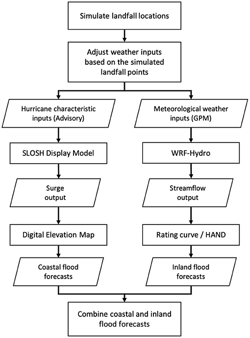
Figure 1. The flow diagram summarizes the overall flood scenario generation methodology which combines both inland and coastal flooding.

3.1. Data Input to Forecasting Models

Inland flood forecasting is driven by the weather forecast, which are output variables from numerical weather models. The meteorological inputs used in this study include precipitation, wind speed, temperature, humidity, and radiation (see Supplementary Table 1) which are the outputs from the Global Forecast System (GFS). The original 13 km output data from GFS was processed to 1 km data by statistical interpolation for the 1-km Weather Research and Forecasting model-Hydrological modeling system (WRF-Hydro) simulation. This regridding was done by NOAA, and we downloaded the 1 km data directly from them. These inputs are then used in the inland flood forecasting model, WRF-Hydro (Gochis et al., 2015, 2018, 2020), which we ran on a local supercomputer. The dynamic input data (atmospheric forcing) were downloaded from the NOAA archive at Renaissance Computing Institute (Alcantara et al., 2017). It should be noted that WRF-Hydro incorporates weather forecasts that are not limited to the characteristics of tropical cyclones.

A center of Tropical Cyclone (TC) is usually defined by the location of the minimum wind field or pressure. We use one of the GFS forecasts which are produced four times per day to define the TC track. We estimate the hourly TC center based on the location of minimum surface wind field. In order to choose one from the multiple GFS forecasts, we need to take the decision-making period (T) into consideration. To provide potential flooding scenarios for impending hurricanes to the decision makers, we utilize the most up-to-date hurricane information by choosing a reference GFS forecast issued T hours before landfall.

When the potential TC might be hazardous, the National Hurricane Center (NHC) issues TC advisories which contain storm information such as position of storm, maximum sustained winds, and potential track. Usually, the advisories are issued in every 6 h. Among the advisories, we choose one advisory as our reference and use the storm information in the advisory as inputs to the storm surge forecasting model, SLOSH Display Program (SDP). We explain the method of choosing a reference advisory in section 3.2. After selecting the reference advisory, among the information contained in the advisory, we collect Saffir-Simpson hurricane intensity and hurricane forward speed as our inputs to the storm surge forecasting model. Two other inputs, the hurricane direction and tide level, are necessary to run SDP. The method for obtaining the inputs from the reference advisory is discussed in section 3.3.

3.2. Scenario Generation Method

We propose a method for scenario generation that considers track error. The tropical cyclone track dominates the distribution of rainfall (Elsberry, 2002; Marchok et al., 2007), which leads to flooding. To create scenarios, we assume that the hurricane landfall location is modeled by a normal random variable, distributed along the Texas coastline, with the mean located at the crossing point between the forecasted hurricane track and the coastline.

In this study, we approximate the Texas coastline with a piecewise linear function with two segments (Figure 2). The first segment is defined by connecting two cities, Port Arthur and Corpus Christi, Texas with a line. The second segment is defined by connecting Corpus Christi and Brownsville, Texas. The GPS coordinates of the three cities are listed in Supplementary Table 3. Note that the distribution is not bounded by the two cities, Brownsville and Port Arthur. The piecewise linear model of the Texas coast described above can be succinctly expressed as follows:

$\begin{array}{ll}f(x)=\{\begin{array}{ll}-17.273x+1709.991\hfill & x\ge {97.39}^{°}W\hfill \\ -0.603x+86.516\hfill & x<{97.39}^{°}W,\hfill \end{array}& (1)\end{array}$

where x is the longitude and f(x) is the corresponding latitude. The longitude of Corpus Christi, which is 97.39° W, is used as the center-point dividing the domain into two intervals. Then, we define the intersection of the hurricane track drawn from the reference GFS forecast and the Texas coastline as the “mean” landfall location.

FIGURE 2

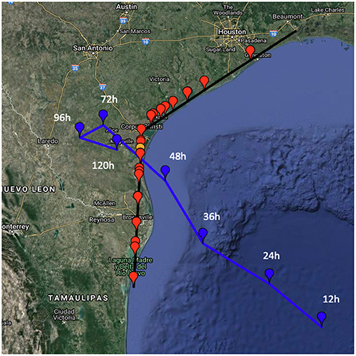
Figure 2. Twenty-five simulated landfall locations for Hurricane Harvey.

The mean landfall location is the reference point for generating inputs for multiple scenarios. Our assumption is that potential landfall locations are normally distributed along the piecewise linear model, with the mean as just described. The standard deviation of the normal distribution can be inferred from the cone of uncertainty. The cone corresponds to the probable track of the TC center. The sizes of cones represent the forecast position errors over the previous 5-year period. The radii of the cone circles in 2017 for the Atlantic basin that are used for the Harvey case study later are given in Supplementary Table 2 (National Hurricane Center, n.d.a).

Since the estimated landfall hour does not perfectly match with one of the forecast periods in Supplementary Table 2, we perform a simple linear interpolation. By calculating the ratio, we compute the corresponding radius of two-thirds cone of uncertainty circle, r = 89 nautical miles. Using the standard normal distribution, we find the standard deviation, σ, of the landfall distribution by using

$\begin{array}{ll}\sigma =\frac{r}{z_{5/6}}& (2)\end{array}$

where z_5/6 is the critical point from a standard normal. Let L be a random variable representing distance from a landfall location to the mean landfall point. Clearly, L = 0 at the mean, and L < 0 for the landfall locations on the left (west) side of the mean location.

Having created a distribution of potential landfall locations, we now describe the stratified sampling method. First, we divide the coastal model into m equiprobable segments. Within each segment, we sample N landfall locations according to the conditional normal distribution on that segment. As mentioned above, once sampled, the resulting mN locations are viewed as being equally likely in later calculations, each occurring with probability of 1/(mN).

For m = 5 and N = 5, the segment boundaries are defined by four quantiles (m₁ to m₄) along the coastline. For example, P(L ≤ m₁) = 1/5. Then, for the first segment we sample five quantiles (p₁ to p₅) from a Uniform (0, 1/5). For the remaining four segments, we also sample quantiles for each segment from a Uniform ((k − 1)/5, k/5), for k = 2,…,5. Overall, we have 25 quantiles which are next translated to landfall locations.

In order to find the physical location of the landfall points, we find z-scores of the sampled quantiles using the standard normal distribution. From the standard normal table, we calculate z_pn, where n = 1,…, mN, and use

$\begin{array}{ll}{l}_n=\sigma z_{p_n}& (3)\end{array}$

to calculate the distance l_n from the mean crossing point in the coastline model, for the corresponding quantile. Finally, the GPS coordinates corresponding to l_n are found by solving for x_n and y_n in the following system:

$\begin{array}{ll}cos(\theta )=\frac{|x_R-x_n|}{l_n}& (4)\end{array}$

$\begin{array}{ll}sin(\theta )=\frac{|y_R-y_n|}{l_n}& (5)\end{array}$

$\begin{array}{ll}\theta =arctan(a_c)& (6)\end{array}$

where a_c is the slope of the coastline that contains the mean location. Here, x_R and y_R are the longitude and latitude of the mean landfall location.

The orange dot in Figure 2 is the mean predicted landfall location for Harvey. Red dots show 25 simulated landfall locations and blue dots indicate the TC center at 12, 24, 36, 48, 72, 96, and 120 h obtained from the reference GFS forecast. Once we have the potential landfall locations, we then run WRF-Hydro to obtain streamflow simulations.

The meteorological conditions at a given time step (hourly here) are used to force the WRF-Hydro model. The atmospheric inputs provided at a 1 × 1 km resolution from the weather models are obtained from the NOAA archive (see Supplementary Figure 1). For each sampled landfall location, we compute the spatial shift, a vector, by using the landfall reference point (the orange point in Figure 2) and the sampled location. Then, for each scenario we shift the atmospheric inputs according to the corresponding vector. To generate comprehensive flood scenarios from hurricanes, we need to combine the inland flooding computations with a coastal flooding model. In our model, we directly combine each inland flooding scenario with a coastal flooding scenario by matching the direction of a hurricane. The detailed steps of aligning the two models are discussed in section 3.3.

3.3. Flood Prediction Methods

3.3.1. Inland Flood Model

We first review our inland flood prediction method. As mentioned at the beginning of section 3.1, we downloaded WRF-Hydro and the corresponding input data from NOAA. Secondly, for scenario generation, we processed the input data to generate 25 sets of input data (as described in section 3.2). Thirdly, the streamflow ouputs from WRF-Hydro were used with HAND datasets to generate inland flood mapping. The details of this third step are described in this section.

WRF-Hydro is an integrated hydrological framework connecting several modules, including the Noah-Multiparameterization Land Surface Model (Noah-MP), a terrain routing module, and a river routing module. The framework enables different models to work with different spatial coordinates. WRF-Hydro simulates typical hydrological processes. The one-dimensional and coarse-resolution land surface model (Noah-MP) is coupled with a two-dimensional and finer resolution terrain routing module, which simulates the hillslope feature for the gravitational redistribution of water. Finally, the river routing module simulates the water flows from upstream to downstream.

The spatial resolution is 1 km for the land surface model and 250 m for the terrain routing module. The river routing module uses a vector-based channel network from the National Hydrography Dataset Plus (NHDPlus) version 2. To estimate the flood level, we apply the Height Above Nearest Drainage (HAND) flood mapping methodology (Liu et al., 2018, 2020; Zheng et al., 2018b). The HAND methodology is a computationally efficient and terrain-based inundation mapping. The HAND is defined as the height of a given location with respect to the nearest stream it drains to. The HAND value of a location is the difference between its elevation and the minimum channel elevation. The resolution of the HAND product is 10 m based on the USGS Digital Elevation Model (DEM) data.

Real-time, street-level inundation mapping is time-consuming. Instead, we process the studied locations in the GIS tool to obtain the corresponding catchment ID and HAND values. This is a one-time approach. Once the WRF-Hydro forecast is produced, we are able to use the pre-processed catchment ID and HAND values to calculate the flood levels.

First, we convert the streamflow to a stage height using a rating curve. The rating curve is a flow-depth relationship that depends on the hydraulic characteristics of the stream channel. Here we use the rating curves included in the HAND product¹. The product provides a table look-up rating curve with a series of 1-foot incremental water levels. We apply linear interpolation to convert streamflow to stage height.

Second, the water level at any given location is calculated from the stage height minus the HAND value if the result is greater than zero. Otherwise, the water level is set to zero if the stage height is smaller than the HAND value. We repeat these steps for each scenario and each location to obtain maximum water levels in 10-day forecast period (from August 24 to September 2, 2017, for Harvey).

3.3.2. Coastal Flood Prediction

We turn our attention to the hydrological model used to predict flooding in the coastal region. When a hurricane makes landfall, the storm brings seawater to the shore, and this phenomenon is called storm surge. To predict the flooding due to the storm surge, we need to know the elevation of the addresses and the storm surge height due to the hurricane. For a particular location, we find the relative surge level above ground by subtracting the elevation from the surge height.

One of the USGS National Geospatial Program products is the 3D Elevation Program (3DEP)². Standard DEMs represent the topographic surface of the earth and contain flattened water surfaces. Each DEM data set is identified by its horizontal resolution and is produced to a consistent set of specifications (United States Geospatial Services, n.d.). We use the standard DEM with the resolution of 1/3 arc-second which is approximately 10 m, and the elevation is referenced to the North American Vertical Datum of 1988 (NAVD88).

There are several storm surge simulation models available to the public. One of the tools that NHC uses to predict storm surges is the SLOSH model. The SLOSH model is a computerized numerical model developed by the NWS to estimate storm surge heights resulting from historical, hypothetical, or predicted hurricanes by taking into account the atmospheric pressure, size, forward speed, and track data (Jelesnianski, 1992). Prior to hurricane landfalls, SLOSH is widely used as a support tool for decision makers in emergency management agencies. To enhance decision making, multiple surge-related products provided by NHC are available.

Using SLOSH, the NHC developed the SDP that supports emergency managers in visualizing storm surge vulnerabilities. The SDP outputs the predicted storm surge levels for fan-shaped basins covering the coastal regions by taking four attributes of a hurricane as input: Saffir-Simpson storm category, storm direction, forward speed, and tide level. A basin is divided into smaller grids and the SDP model predicts the surge height above the sea level for each grid. The model outputs storm surge heights for a particular area in feet above the reference sea level NAVD88. To interpret the surge level, users need to subtract the elevation from the surge heights as discussed earlier.

For our surge forecasting tool, we use the SDP. For a particular region, a user can input the four attributes of the hurricane to obtain the Maximum Envelope of Water (MEOW)³ which provides a worst-case basin snapshot of surge levels for a particular storm category, forward speed, hurricane direction, and tide level. Since the MEOW highlights the worst case of an expected hurricane, it is a time-independent concept, unlike the WRF-Hydro stage height output. The downside of using the time-independent measure is that the duration of high waters is ignored. The SDP output does not indicate how long the storm surge covers the impacted areas. Nonetheless, the MEOW is “robust” from the view point of optimization because it based on the worst-case outcome for a particular storm, instead of, for example, the average outcome or a probability distribution over multiple outcomes.

Before generating storm surge scenarios, we need to study the input parameters of the SDP in more detail. As mentioned earlier, there are four input parameters for the MEOW product: storm direction, intensity, tide level, and forward speed. The available surge outputs in SDP depend on each basin. For the Galveston basin, which we use for our case study, there are nine cardinal trajectory directions available from west-southwest to east-northeast (WSW, W, WNW, NW, NNW, N, NNE, NE, and ENE). We assume that a storm may come in one of nine directions with a fixed storm intensity, tide level, and forward speed. To determine the incoming storm's characteristics other than direction, we study the reference hurricane advisory provided by the NHC. The forecast advisory issued by the NHC provides present movement speed, direction, hurricane track, and maximum wind speed in time series.

To choose the storm intensity represented by the Saffir-Simpson hurricane wind scale, we look at the expected maximum wind speed within the 5-day hurricane forecast by the NHC. According to the 5-day Forecast Track and Watch/Warning Graphic of the reference advisory, Advisory 14 (see Supplementary Figure 1), the maximum sustained wind speed is listed as 74–110 mph, which can be easily converted to Category 2 of Saffir-Simpson category scale. In the SDP, there are two tide levels available: mean and high tide. Since the tide hours vary by location and SDP does not generate the time-specific output, we assume that the storm makes landfall at the high-tide level. There are three forward speed categories: 5, 10, 15 mph. The forward speed from the advisory is 2 mph. We choose the closest forward speed category, 5 mph, among the three options.

Figure 3 shows a SDP output generated from a Category 2 storm traveling in north direction with forward speed of 5 mph at high tide. Within the study region colored in gray, the hospital and nursing home locations are indicated by red dots and blue triangles, respectively. The elliptical shaped mesh grids are used to output surge levels, and the resolution of each cell ranges from tens to hundreds of meters to a kilometer or more. A darker color indicates a higher surge level.

FIGURE 3

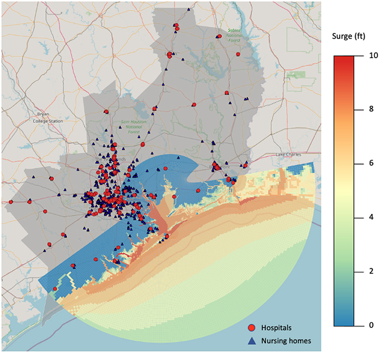
Figure 3. Storm surge output from SDP generated with a Category 2 storm traveling in north direction with forward speed of 5 mph at high tide shows impact on the hospitals (red dots) and nursing homes (blue triangles) in our region of interest.

To cover the hospital locations in our interest region, we collect one-degree blocks of DEM spanning from 29 to 32° N and 94 to 97° W. We use a GIS software, QGIS 3.8, to extract the elevation of hospital locations.

3.3.3. Combined Flood Prediction

Now, we are able to combine each inland flooding scenario with a coastal flooding scenario by matching the direction of a hurricane. For each hurricane scenario, we are able to define the hurricane direction by connecting the sampled landfall location and a reference hurricane center point which is defined as the current hurricane location (note that this is different from the earlier reference point, the mean predicted landfall location). To find the current hurricane location we use the GFS forecast generated at 00:00 UTC on August 24th. Once we have the hurricane direction for an inland flooding hurricane scenario, we determine the closest storm direction in the coastal flooding model. This allows us to produce a set of inundated locations due to storm surge. To produce the set of all flooded locations for a particular scenario we then take the union of the set of locations flooded according to the inland model and the set of locations flooded according to the coastal (storm surge) models. Note that our methodology does not take into account combined inland and coastal flooding effects. This is an important direction for future research.

For example, in Figure 2, the southern-most landfall location in the simulated inland flooding model is at (24.50° N, 97.58° W). The closest storm direction in SDP to the direction generated by connecting the reference hurricane center point at 12 h and the southern-most landfall location is the west direction. The 25 landfall locations and their matching directions are shown in Table 1.

TABLE 1

Table 1. Landfall locations and matching storm surge directions.

4. Validation

Our model validation is performed using the High Water Marks (HWMs) collected by the USGS after Hurricane Harvey⁴. We remove HWM locations outside the region of interest or in catchments of lakes and reservoirs, in which the current WRF-Hydro-HAND methodology cannot provide flooding information. The measurements we used were the maximum HWM reading at each site having an excellent, good, or fair reading. Figure 4 displays 750 unique HWM sites within our study region. We observe that many HWM sites are concentrated near the center of the figure, close to central Houston.

FIGURE 4

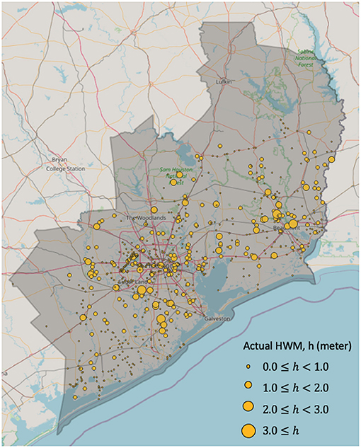
Figure 4. The circles represent the actual HWMs of the 750 sites within the CMOC region.

We evaluate the accuracy of our methodology in flood prediction in capturing using the following rates:

$\begin{array}{ll}\text{Hit Rate (HR)}=P(M_1|H_1)=\frac{P(M_1\cap H_1)}{P(H_1)}& (7)\end{array}$

$\begin{array}{ll}\text{False Positive Rate (FPR)}=P(M_1|H_0)=\frac{P(M_1\cap H_0)}{P(H_0)}.& (8)\end{array}$

From a statistical viewpoint, we interpret M₀ as the event that the model predicted a site to be dry (0) and M₁ as the event that the model predicted a site to be wet (1) (i.e., flooded). Similarly, H₀ and H₁ indicate events that the site is actually dry (0) and wet (1) by the HWM. Thus, P(H₁) is the number of flooded sites with HWM value greater than threshold level divided by the total number of sites. The threshold is set as 0 m. Unlike the false alarm ratio used in Wing et al. (2017), we use the false positive rate which directly represents the probability of Type 1 error. If the flood predictions are used in evacuation decisions, then it is likely that the false negative rate is more critical than the false positive rate since the consequences of not evacuating a location that floods are usually worse than unnecessarily evacuating. The false negative rate can be easily obtained by subtracting the hit rate from one.

Column (a) in Table 2 shows the hit rates and false positive rates by computing over all 750 HWM sites. The hit rate and false negative rate improve in the middle scenarios (around L11–L16, around L13) and tend to decrease for landfall locations farther from the mean path (farthest ones are L1 and L25). The false positive rates are higher in the middle scenarios, suggesting that the model tends to overestimate flooding in scenarios where the landfall location is close to the mean path. Note that both rainfall and storm surge are expected to be most severe in the region of interest, in the middle scenarios. In turn, this induces an increase in both the hit rate and an overestimation of flooding in more HWM sites.

TABLE 2

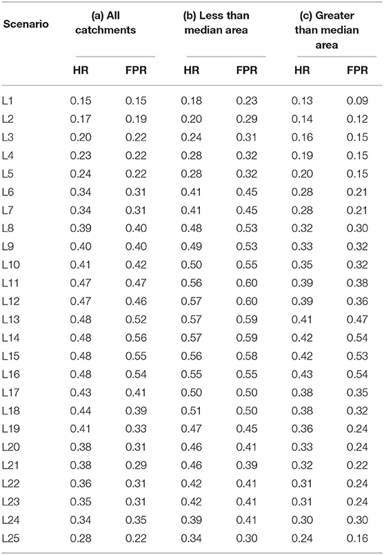
Table 2. The comparison of hit rates (HR) and false positive rates (FPR) for 25 hurricane scenarios.

In order to assess the effect of catchment size on accuracy, we divide the HWM sites by the area of encompassing catchments. We find the median catchment area and evaluate the model under both metrics for sites within catchments smaller than the median. We perform the same calculation for the remaining sites within larger catchments. Among the 750 sites, there are 318 sites within a catchment area smaller than the median area of 9.26 km². The remaining 432 sites are within the larger catchments. In Columns (b) and (c) of Table 2, we compare the two metrics obtained from the two types of sites. A similar trend in hit rates and false positive rates is observed. In both cases, the hit rates improve in the middle scenario whereas the false positive rates are worse. Comparing the overall metrics of (a), (b), and (c), the hit rate is the best in the sites in smaller catchments whereas the false positive rate is worse. This suggests that the sensitivity of the flood prediction model is greater for smaller catchments.

In order to provide some graphical intuition for the results of the HWM evaluation, we compare our WRF-Hydro-HAND model results with USGS-FEMA flood-inundation maps (Watson et al., 2018), which are created using HWMs and Lidar elevation data. The modeled results are created with the maximum streamflow in the predicted period. Figure 5 shows an underestimated case at Reach 1520007 on the East Fork San Jacinto River and its corresponding NHDPlus catchment in the black boundary. The inundation extent in L13 and L25 are similar but smaller than the inundation as estimated from USGS-FEMA. Furthermore, the results from L13 and L25 are very similar to one generated with the National Water Model reanalysis product, which is driven by observed precipitation (results not shown). In contrast, the inundation extent in L1 is small because the precipitation in this scenario is the smallest in our studied region due to the simulated landfall location.

FIGURE 5

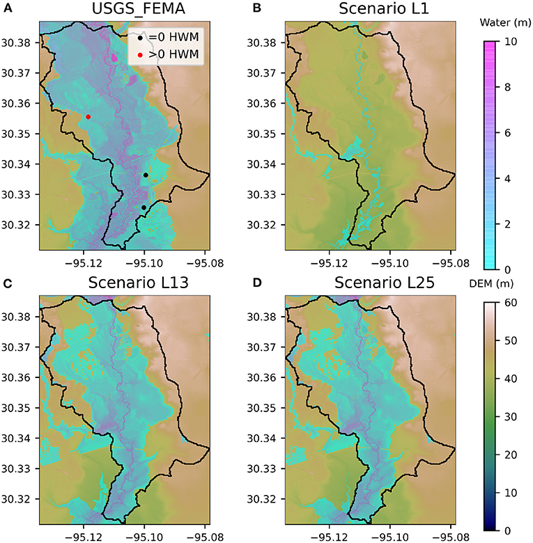
Figure 5. Comparison of inundation maps: (A) observed—based on USGS-FEMA, (B–D) predicted maximum inundation from scenarios.

5. Case Study

5.1. Study Region and Locations

In our case study, we focus on hospitals and nursing homes in the southeast Texas region. SETRAC, the Southeast Texas Regional Advisory Council, is responsible for coordinating patient evacuation in 25-county service region in and around Houston. For example, during Hurricane Harvey in 2017, SETRAC coordinated 773 patient movement missions that evacuated 1,544 patients from 24 hospitals. As such, SETRAC provided important guidance in formulating the case study described here. To choose hospitals and nursing homes from the greater Houston region, we utilize the datasets from the Homeland Infrastructure Foundation-Level Data (HIFLD)⁵. We choose the facilities by filtering the datasets for Texas and the 25 counties, and by selecting locations with status “open.” After filtering the datasets, we find 176 hospitals and 716 nursing homes in our region of interest. Among the 176 hospitals, we remove six hospitals and 14 nursing homes that are not in the catchments of rivers (Liu et al., 2018; Zheng et al., 2018a). The remaining 170 hospitals and 702 nursing homes locations are marked in red dots and blue triangles respectively in Figure 3.

To provide potential flood scenarios so that SETRAC can plan patient evacuation missions before the hurricane landfall, the 48 h window before landfall is important. When a hurricane is too close to the coast, the road network is expected to be congested because of the evacuating general population. The mobility of emergency medical service vehicles is also restricted by the wind speed. The 48 h window provides assurance that their evacuation operations is minimally affected by the approaching hurricane while providing the most up-to-date information for generating potential flood maps.

5.2. Inland Flooding Analysis

Our modeling domain of WRF-Hydro is the Texas-Gulf region with the watershed boundary of the USGS 2-digit Hydrologic Unit Code (HUC-2 region 12) with approximately 471,000 km². The domain consists of 67,294 NHDPlus river reaches and catchments (Figure 6). The hospitals and nursing homes in this study are scattered in the area, which is mainly at the lower part of the Colorado River, Brazos River, Trinity River, Neches River, and Sabines River watersheds. Sixty five percent of the studied locations are in the San Jacinto River watershed.

FIGURE 6

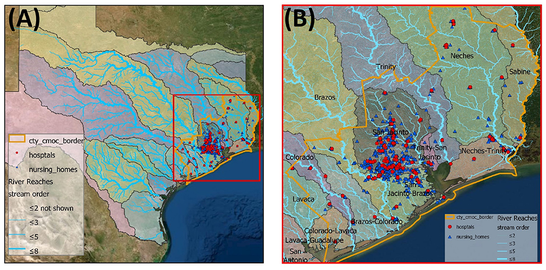
Figure 6. The WRF-Hydro modeling domain within the Texas-Gulf Region. (A) Entire modeling domain that consists NHDPlus reaches, (B) the region of the hospitals and nursing homes (CMOC).

The performance of hydrological simulation is sensitive to the precipitation amount and pattern. Figure 7 shows the 10-day (from August 24 to September 2, 2017) accumulated precipitation with our studied region highlighted. Here we use the precipitation products from the NASA Global Precipitation Measurement (GPM) (Huffman et al., 2015) as “true” precipitation. Generally, the satellite-based observation shows that most of the precipitation is concentrated in the Houston area. The precipitation forecasts, which are the inputs for WRF-Hydro simulation, are generated on August 24. Compared with GPM, the precipitation forecast predicts that the hurricane would drop heavier rainfall as it makes its first landfall, and the rainfall happens along with the track. It is not surprising that the forecast produced on August 24 is not able to capture the slow movement of the hurricane over eastern Texas. However, among the simulated 25 scenarios, in eleven scenarios, total precipitations in the CMOC region are higher than the precipitation of the mean path scenario (L13). The highest 10-day accumulated precipitation in the CMOC region among all scenarios is 457.26 mm which is experienced in Scenario L21. Total estimated precipitations in all scenarios are lower than the observed precipitation of 549.72 mm.

FIGURE 7

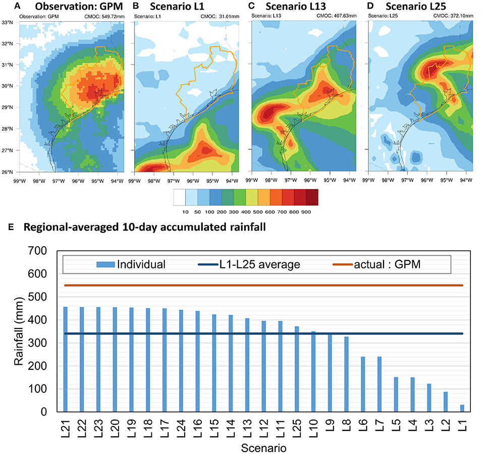
Figure 7. Comparison of 10-day accumulated rainfall in the CMOC region between 25 scenarios (model) and GPM (observation). (A) Spatial pattern of GPM, (B) results from scenario L1, (C) results from L13, (D) results from L25, (E) CMOC regional-averaged rainfall from scenarios using weather predictions and from satellite-based observations from GPM from August 24 to September 2, 2017.

As part of the Gulf Coastal Plains, the terrain of the majority of the study region is flat, especially for the area close to the coastline (see Supplementary Figure 3). The city of Houston is mostly urbanized and flat. Twenty-two hospitals and ten nursing homes are located in one catchment, Brays Bayou (Reach ID 1440385). The HAND values of the address points for hospitals and nursing homes range from 9.45 to 14.40 m, which means that all studied locations are predicted to be flooded when the water level in the channel of Brays Bayou is larger than 14.40 m. Our results suggest that 17 studied locations (13 hospitals and 4 nursing homes in the catchment of Brays Bayou) are estimated to be flooded in a worst-case scenario. These 17 locations have HAND values lower than 11.87 m, which is the maximum predicted stage height.

5.3. Coastal Flooding Analysis

For the 25 flood scenarios, four SDP outputs contribute to the flood mapping. Table 1 shows that the SDP output generated with the west direction occurs in just one scenario while the west-northwest, northwest and north-northwest directions appear 7, 13, and 4 scenarios, respectively. In the Galveston basin, the maximum surge above the sea level (3.47 m) occurs in the storm surge forecast generated with the northwest direction.

There are nine locations that have mean inundation level greater than the threshold level of 0 m. Among the nine, there are two hospitals (h144, h146) and seven nursing homes (n597, n608, n610, n612, n615, n640, n662). Two nursing homes (n640, n662) are located near Port Arthur, TX, while the rest of the locations are in the Galveston area. Supplementary Table 4 summarizes storm surge statistics, elevation above sea level (NAV88) and the inundation level of the nine hospitals. There are seven locations (h33, n298, n574, n603, n607, n622, n623) in which the elevation is greater than forecasted surge levels in every scenario resulting the mean inundation level as 0.

5.4. Combined Flooding Analysis

Recall that there are 25 flood sets that are formed by taking the union of the inland and coastal flooding sets. With a threshold level of 0 m, the minimum number of flooded locations (21 locations) is realized in Scenario L1. The number of flooded location is maximum (153 locations) in Scenario L15. The mean number of flooded locations from the 25 scenarios is approximately 92. When the landfall location is expected to be at the southern-most location, the number of flooded hospitals is minimal. When the hurricane landfall location is toward the center of the distribution, the model generates the maximum number of flooded hospitals.

In total, there are 215 locations that experience flooding in at least one of the 25 scenarios. Figure 8A shows the mean flood levels (measured above ground level) of the 215 flooded facilities. The darker color indicates a higher mean flood level. Examining the locations of the flooded facilities in the figure, we are able to see that majority of the flooded locations are located in inland. Figure 8B shows the locations and their probability of flooding (indicating a positive flood level). Darker colors indicate higher probability of flood level being >0. Comparing the two figures, we highlight that locations with higher flood level are likely to have higher probability of flooding.

FIGURE 8

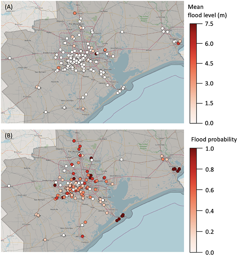
Figure 8. (A) Mean flood levels (calculated from 25 scenarios)—darker colors indicate higher mean flood levels. (B) Flood probabilities—darker colors indicate higher probabilities of flooding (i.e., flood level being positive).

There are two locations (n640, n662) that are both impacted by streamflow and storm surge. In our analysis, we assume no interaction between streamflow and storm surge, and define their flood level with higher flood level obtained from either streamflow or storm surge. In both locations, flooding due to streamflow generates higher water level above ground. The mean flood levels of the two locations (n640, n662) from storm surge are (0.555, 0.623 m) while the flood levels from streamflow are (2.923, 2.947 m), respectively.

Table 3 shows how the number of flooded locations changes with increasing the flood threshold level. The mean number of flooded locations due to coastal flooding approaches 0 when the threshold is increased from 0 to 1 m. The maximum number of flooded locations for threshold levels 0.0 and 1.0 m occurs in Scenario L15. When the threshold level is 0.5 m, the number of flooded locations is maximum in Scenario L14. For all threshold levels, the number of flooded locations is minimized in Scenario L1.

TABLE 3

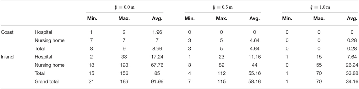
Table 3. Number of flooded locations in different threshold levels (ξ).

Now, instead of looking both hospital and nursing home locations, we only look at a subset, the hospitals in the region, to provide more detailed results a decision maker can use with an access to our probabilistic scenario-based analysis. For example, decision makers who plan for mitigation actions for hospital flooding should consider not only the flood probability but also the various statistics of flood levels because the capability of each hospital to withstand flooding is different. As a sampling of such analysis, Table 4 shows 45 hospital locations subjected to flooding in the 25 scenarios. It shows flooding probabilities of hospital locations and their minimum, maximum, and average flood height. According to the analysis, Hospitals h72 and h151 are expected to suffer from the most severe flooding. Three hospitals (h144, h150, h151) are expected to be flooded in every scenario. The flood probability of Hospital h150 is 1, but the average and maximum flood levels are 0.28 and 0.84 m. Contrast that to Hospital h35, with the average and maximum flood levels at 2.21 and 5.90 m, respectively, and with 0.72 probability of flooding. Although Hospital h150 is expected to be flooded in every scenario, the degree of flooding in this location may not be severe enough to plan for an evacuation. In comparison, due to the magnitude of the expected flood level, it might be a good idea to prepare for flooding (say evacuate) for Hospital h35.

TABLE 4

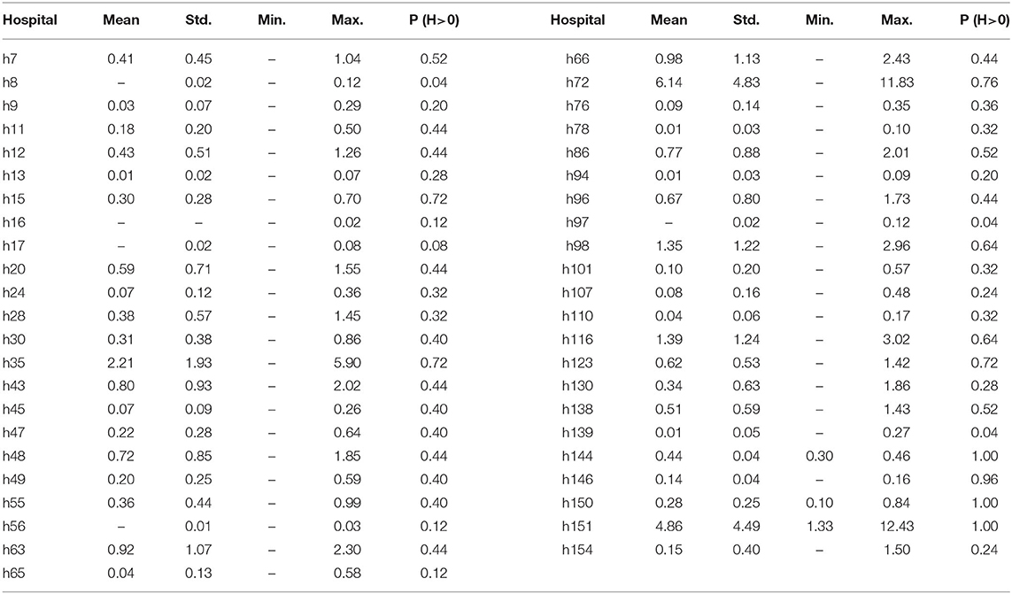
Table 4. Flood statistics (in meters) and probability of flood level (H) greater than zero for hospitals in the region of interest.

In flood level forecasting, it is useful for evacuation decision makers to ask how often the flood level is above a particular level. Table 5 shows the complementary cumulative distributions, P_s(H > h), of flood level random variable, H, of 45 flooded hospitals (s). In the table, the flood level values (h), from 0 to 4 m with an increment of 0.5, are chosen to describe the distributions. The probability of Hospital h45 to have flood level >0 is 0.40, and it does not expect a flood level above 0.5 m. This indicates, in any scenario, the maximum flood level at h45 does not exceed 0.5 m. On the other hand, the probabilities that Hospital h72 to have flood level >2 and 4 m are 0.68 and 0.60, respectively. From the table, we can also make inferences on the forecasted flood level distribution. For Hospitals h48 and h96, we see that the forecasted flood levels lie in the intervals (0, 0.5m] and (1.5, 2m]. When dealing with a bimodal flood level distribution, such analyses are more useful than looking at the mean and standard deviation of flood levels, as in Table 4.

TABLE 5

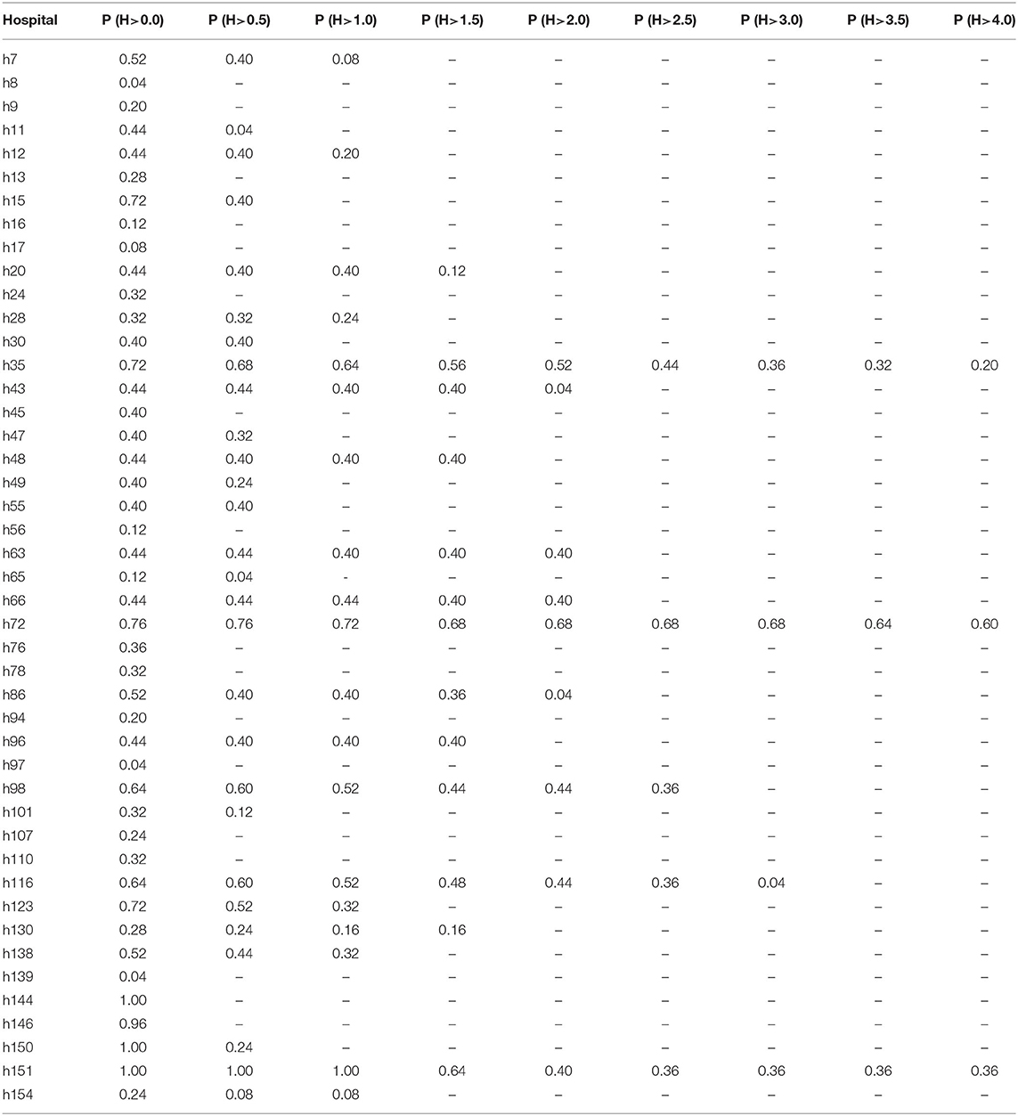
Table 5. Complementary cumulative distribution functions of flood level (m) at hospitals.

Depending on the flood prevention structures in each hospital, one may be comfortable with certain levels of flood level during flooding events. Another factor in an evacuation decision is the risk preference of the decision maker. The hospital evacuation decision is a unique decision making process because the decision maker is expected to make balanced decisions between financial and medical losses caused by evacuating and unfortunate consequences from not evacuating.

The number of flooded hospitals induced by the mean path scenario (L13) is 39 while the mean number of flooded hospital over all scenarios is 19.2. We generate flood level distribution of each hospital from 25 scenarios. Supplementary Figure 3 Shows the positions of flood level from mean path (marked as “x”) at each hospital's flood level distribution. There are nine hospitals at which the flood level from mean path is at or below the median. Similarly, when the flood levels from mean path are compared to the average of each hospital's flood level (in dots), there are nine hospitals whose average flood levels from the scenarios are greater than the mean path flood levels. There are 39 hospitals whose average flood levels from the scenarios are greater than the median flood levels suggesting distributions to be right-skewed.

6. Future Work

In preparing for future hurricanes, government agencies continue to rely on flood models that are not designed for specific forthcoming hurricanes, and the comprehensive flood mapping for both inland and coastal area is still in need. In this paper, we have developed a probabilistic scenario generation scheme for hurricane flooding. By sampling landfall locations of an impending hurricane, we simulate inland flooding scenarios and align each of them with a coastal flooding scenario based on the hurricane directions. Considering Hurricane Harvey as our instance, by using the data obtained two days before the hurricane, the uncertainty in hurricane-induced flooding is quantified. We have shown how the probabilistic flood scenarios can support disaster response decisions such as hospital evacuation planning. For this study, we have attempted to replicate flooding scenarios for Hurricane Harvey. We plan to apply our flood scenario generation to multiple hurricane events and compare our predictions with the high-water marks and perform calibration. In the model validation steps, it is suggested that the hit rate of flooding improves when the model is applied to smaller catchments. Incorporating the higher resolution water routing model and enhancing the land surface model in runoff routing due to precipitation will improve the accuracy of the overall methodology.

We plan to reinforce technical aspects of scenario generation. The current method involves locational shifting of meteorological inputs such as precipitation based on the possible hurricane landfall location. We believe that our methodology can take advantage of the improvements in ensemble meteorological forecasting and high performance computing, to achieve an ensemble-based flood forecasting taking advantage of potential cross-disciplinary approaches. We also intend to improve the current technique of data assimilation by calibrating hydrological model outputs with high water mark observations. Moreover, to improve the storm surge-side of the forecasting in flood prediction, we plan to enhance the methods for accounting for more sources of uncertainty. Finally, the scenario generation approach can be integrated more directly with the decision making and resource allocation models, giving the involved decision makers better tools to quantify uncertainty and to make more informed mitigation and preparedness decisions.

Data Availability Statement

The raw data supporting the conclusions of this article will be made available by the authors, without undue reservation.

Author Contributions

All authors listed have made a substantial, direct and intellectual contribution to the work, and approved it for publication.

Funding

NSF grant: CoPe EAGER: Addressing Human-Centric Decision-Making Challenges from Coastal Hazards via Integrated Geosciences Modeling and Stochastic Optimization supported the publication fee along with the support for all the authors. This research was also funded by a grant from the Planet Texas 2050 program at the University of Texas at Austin.

Conflict of Interest

The authors declare that the research was conducted in the absence of any commercial or financial relationships that could be construed as a potential conflict of interest.

Supplementary Material

The Supplementary Material for this article can be found online at: https://www.frontiersin.org/articles/10.3389/fclim.2021.610680/full#supplementary-material

Footnotes

1. ^https://cfim.ornl.gov/data/

2. ^https://viewer.nationalmap.gov/basic/

3. ^https://www.nhc.noaa.gov/surge/meowOverview.php

4. ^https://stn.wim.usgs.gov/FEV/

5. ^https://hifld-geoplatform.opendata.arcgis.com/datasets/hospitals

References

Alcantara, M. A. S., Crawley, S., Stealey, M. J., Nelson, E. J., Ames, D. P., and Jones, N. L. (2017). Open water data solutions for accessing the National Water Model. Open Water J. 4:3.

Google Scholar

Blake, E. S., and Zelinsky, D. A. (2018). National Hurricane Center Tropical Cyclone Report: Hurricane Harvey. Technical report, National Hurricane Center.

Google Scholar

Contento, A., Xu, H., and Gardoni, P. (2018). “A physics-based transportable probabilistic model for climate change dependent storm surge,” in Routledge Handbook of Sustainable and Resilient Infrastructure. 1st Edn, ed P. Gardoni (New York, NY: Routledge), 662–682. doi: 10.4324/9781315142074-34

CrossRef Full Text | Google Scholar

Dietrich, J., Zijlema, M., Westerink, J., Holthuijsen, L., Dawson, C., Luettich, R. Jr, et al. (2011). Modeling hurricane waves and storm surge using integrally-coupled, scalable computations. Coast. Eng. 58, 45–65. doi: 10.1016/j.coastaleng.2010.08.001

CrossRef Full Text | Google Scholar

Elsberry, R. L. (2002). Predicting hurricane landfall precipitation: optimistic and pessimistic views from the symposium on precipitation extremes. Bull. Am. Meteorol. Soc. 83, 1333–1339. doi: 10.1175/1520-0477(2002)083<1333:PHLPOA>2.3.CO;2

CrossRef Full Text | Google Scholar

Gochis, D., Barlage, M., Cabell, R., Casali, M., Dugger, A., FitzGerald, K., et al. (2020). The WRF-Hydro®Modeling System Technical Description (Version 5.1.1). doi: 10.5281/zenodo.3625238

CrossRef Full Text | Google Scholar

Gochis, D., Barlage, M., Dugger, A., FitzGerald, K., Karsten, L., McAllister, M., et al. (2018). The WRF-Hydro Modeling System Technical Description (Version 5.0). doi: 10.5065/D6J38RBJ

CrossRef Full Text | Google Scholar

Gochis, D., Yu, W., and Yates, D. (2015). The WRF-Hydro Model Technical Description and User's Guide, Version 3.0. doi: 10.5065/D6DN43TQ

CrossRef Full Text | Google Scholar

Huffman, G., Stocker, E., Bolvin, D., Nelkin, E., and Tan, J. (2015). GPM IMERG Final Precipitation L3 1 Day 0.1 Degree x 0.1 Degree V06. Greenbelt, MD.

Jelesnianski, C. P. (1992). SLOSH: Sea, Lake, and Overland Surges from Hurricanes, Vol. 48. U.S. Department of Commerce, National Oceanic and Atmospheric Administration, National Weather Service.

PubMed Abstract | Google Scholar

Jia, G., and Taflanidis, A. A. (2013). Kriging metamodeling for approximation of high-dimensional wave and surge responses in real-time storm/hurricane risk assessment. Comput. Methods Appl. Mech. Eng. 261, 24–38. doi: 10.1016/j.cma.2013.03.012

CrossRef Full Text | Google Scholar

Kim, S., Melby, J. A., Nadal-Caraballo, N. C., and Ratcliff, J. (2015). A time-dependent surrogate model for storm surge prediction based on an artificial neural network using high-fidelity synthetic hurricane modeling. Nat. Hazards 76, 565–585. doi: 10.1007/s11069-014-1508-6

CrossRef Full Text | Google Scholar

Liu, Y. Y., Maidment, D. R., Tarboton, D. G., Zheng, X., and Wang, S. (2018). A CyberGIS integration and computation framework for high-resolution continental-scale flood inundation mapping. JAWRA J. Am. Water Resour. Assoc. 54, 770–784. doi: 10.1111/1752-1688.12660

CrossRef Full Text | Google Scholar

Liu, Y. Y., Tarboton, D. G., and Maidment, D. R. (2020). Height Above Nearest Drainage (HAND) and Hydraulic Property Table for CONUS - Version 0.2.1. (20200601). Oak Ridge Leadership Computing Facility.

Google Scholar

Mandli, K. T., and Dawson, C. N. (2014). Adaptive mesh refinement for storm surge. Ocean Model. 75, 36–50. doi: 10.1016/j.ocemod.2014.01.002

CrossRef Full Text | Google Scholar

Marchok, T., Rogers, R., and Tuleya, R. (2007). Validation schemes for tropical cyclone quantitative precipitation forecasts: evaluation of operational models for U.S. landfalling cases. Weath. Forecast. 22, 726–746. doi: 10.1175/WAF1024.1

CrossRef Full Text | Google Scholar

National Hurricane Center (n.d.a). NHC GIS Archive - Tropical Cyclone Advisory Forecast. Available online at: https://www.nhc.noaa.gov/gis/archive_forecast_results.php?id=al09&year=2017&name=Hurricane%20HARVEY

National Hurricane Center (n.d.b). Sea Lake Overland Surge from Hurricanes (SLOSH). Available online at: https://slosh.nws.noaa.gov/slosh/index.php?L=7#intro

National Oceanic Atmospheric Administration (2018). Inland Flooding: A Hidden Danger of Tropical Cyclone. Available online at: https://www.noaa.gov/stories/inland-flooding-hidden-danger-of-tropical-cyclones

NOAA National Centers for Environmental Information (NCEI) (2020). U.S. Billion-Dollar Weather and Climate Disasters. Available online at: https://www.ncdc.noaa.gov/billions/

United States Geospatial Services (n.d.). About 3DEP Products & Services. Available online at: https://www.usgs.gov/core-science-systems/ngp/3dep/about-3dep-products-services

Watson, K., Welborn, T., Stengel, V., Wallace, D., and McDowell, J. (2018). Data Used to Characterize Peak Streamflows and Flood Inundation Resulting From Hurricane Harvey of Selected Areas in Southeastern Texas and Southwestern Louisiana, August-September 2017: U.S. Geological Survey Data Release. doi: 10.3133/sir20185070

CrossRef Full Text

Westerink, J. J., Luettich, R. Jr, Blain, C., and Scheffner, N. W. (1994). ADCIRC: An Advanced Three-Dimensional Circulation Model for Shelves, Coasts, and Estuaries. Report 2. User's Manual for ADCIRC-2DDI. Technical report, ARMY Engineer Waterways Experiment Station, Vicksburg, MS.

Google Scholar

Wing, O. E., Bates, P. D., Sampson, C. C., Smith, A. M., Johnson, K. A., and Erickson, T. A. (2017). Validation of a 30 m resolution flood hazard model of the conterminous United States. Water Resour. Res. 53, 7968–7986. doi: 10.1002/2017WR020917

CrossRef Full Text | Google Scholar

Zheng, X., Maidment, D. R., Tarboton, D. G., Liu, Y. Y., and Passalacqua, P. (2018a). GeoFlood: Large-scale flood inundation mapping based on high-resolution terrain analysis. Water Resour. Res. 54, 10–13. doi: 10.1029/2018WR023457

CrossRef Full Text | Google Scholar

Zheng, X., Tarboton, D. G., Maidment, D. R., Liu, Y. Y., and Passalacqua, P. (2018b). River channel geometry and rating curve estimation using height above the nearest drainage. JAWRA J. Am. Water Resour. Assoc. 54, 785–806. doi: 10.1111/1752-1688.12661

CrossRef Full Text | Google Scholar