 Peter Köhler
- Alfred-Wegener-Institut Helmholtz-Zentrum für Polar-und Meeresforschung (AWI), Bremerhaven, Germany
The CO2 removal model inter-comparison (CDRMIP) has been established to approximate the usefulness of climate mitigation by some well-defined negative emission technologies. I here analyze ocean alkalinization in a high CO2 world (emission scenario SSP5-85-EXT++ and CDR-ocean-alk within CDRMIP) for the next millennia using a revised version of the carbon cycle model BICYCLE, whose long-term feedbacks are calculated for the next 1 million years. The applied model version not only captures atmosphere, ocean, and a constant marine and terrestrial biosphere, but also represents solid Earth processes, such as deep ocean CaCO3 accumulation and dissolution, volcanic CO2 outgassing, and continental weathering. In the applied negative emission experiment, 0.14 Pmol/yr of alkalinity—comparable to the dissolution of 5 Pg of olivine per year—is entering the surface ocean starting in year 2020 for either 50 or 5000 years. I find that the cumulative emissions of 6,740 PgC emitted until year 2350 lead to a peak atmospheric CO2 concentration of nearly 2,400 ppm in year 2326, which is reduced by only 200 ppm by the alkalinization experiment. Atmospheric CO2 is brought down to 400 or 300 ppm after 2730 or 3480 years of alkalinization, respectively. Such low CO2 concentrations are reached without ocean alkalinization only after several hundreds of thousands of years, when the feedbacks from weathering and sediments bring the part of the anthropogenic emissions that stays in the atmosphere (the so-called airborne fraction) below 4%. The efficiency of carbon sequestration by this alkalinization approach peaks at 9.7 PgC per Pmol of alkalinity added during times of maximum anthropogenic CO2 emissions and slowly declines to half this value 2000 years later due to the non-linear marine chemistry response and ocean-sediment processes. In other words, ocean alkalinization sequesters carbon only as long as the added alkalinity stays in the ocean. To understand the basic model behavior, I analytically explain why in the simulation results a linear relationship in the transient climate response (TCR) to cumulative emissions is found for low emissions (similarly as for more complex climate models), which evolves for high emissions to a non-linear relation.
1. Introduction
Most approaches for negative CO2 emissions, especially when based on oceanic processes, are still future technologies. This implies, that we do not know in detail how efficient different approaches might work in reality. Furthermore, unknown are also difficulties we need to overcome during potential implementations, and how we minimize in detail unwanted side effects (e.g., Keller et al., 2014; Committee on Geoengineering Climate, 2015; The Royal Society, 2018). For an approximation of the intended climate mitigation, however, some simulation protocols have been established within the carbon dioxide removal model intercomparison project (CDRMIP), part of CMIP6 (Keller et al., 2018), to allow intermodel comparisons. Within the suite of proposed CDR experiments exists the “ocean alkalinization in a high CO2 world” scenario (CDR-ocean-alk). While most recent studies on negative emission technologies—and most contributions to CDRMIP—focus on centennial time scales (e.g., Keller et al., 2014; González and Ilyina, 2016; Lenton et al., 2018; Beerling et al., 2020), I here concentrate on long-term effects (thousands to millions of years) by analyzing simulations of CDR-ocean-alk performed with only one simple model, the carbon cycle box model BICYCLE.
The long-term fate of fossil fuel emissions have been investigated in details with models of different complexities. Models differ in detail how the different feedbacks amplify or dampen the anthropogenic emissions (e.g., Archer et al., 2009). However, the common understanding can be summarized as follows:
• An anthropogenic-induced CO2 anomaly in the atmosphere is in pulse experiments after a century (a millennium) reduced to <50% (to ~20%) (Joos et al., 2013) due to the CO2 uptake by the ocean and the vegetation, the later mainly due to the CO2 fertilization (e.g., Haverd et al., 2020).
• The positive temperature feedback (the fossil fuel-induced global warming) leads to a warming of the surface ocean and via a then lower solubility of CO2 in water (Henry's law) to a rise in atmospheric CO2 (Weiss, 1974).
• The carbonate compensation (e.g., Archer et al., 1997) working on multi-millennial time scales is a negative feedback, also called sediment feedback. It implies that the anthropogenic CO2 entering the ocean reduces the deep ocean carbonate ion concentration, consequently dissolving CaCO3 due to calcite and aragonite undersaturation, leading to a rise in marine alkalinity and dissolved inorganic carbon (DIC) in the ocean. These changes in the carbonate chemistry allow an enhanced oceanic uptake of CO2 from the atmosphere, roughly reducing the airborne fraction of anthropogenic CO2 by a factor two down to ~10%.
• On even longer time scales, high atmospheric CO2 concentration leads via the negative weathering feedback to a further lowering of the CO2 anomaly (e.g., Colbourn et al., 2015).
These airborne fractions given above are only rough estimates, since results are highly model dependent and also to some extend a function of the amount of emitted fossil fuels (Archer et al., 2009; Joos et al., 2013). They are typically calculated from pulse-response experiments, in which a well-defined amount of carbon (e.g., 100, 1,000, or 5,000 PgC) is injected in the atmosphere in 1 year or so, while already simulations considering the temporal evolution of the historic anthropogenic CO2 emissions lead to a slightly different response of the carbon cycle (Jones et al., 2013). A nice overview of the time scales of the different processes reducing anthropogenic-induced CO2 in the atmosphere is given in Lord et al. (2016).
The results presented here make use of the achieved understanding of these processes and feedbacks and focus on how long-term alkalinization might mitigate the impact of high CO2 emissions. To set this into context to results obtained with more complex models, a good understanding of control simulations without alkalinization is necessary. I will therefore also analyze the implemented temperature, weathering, and sediment feedbacks embedded in the BICYCLE model, and derive an analytical understanding of the TCR to cumulative emissions within the applied model.
2. Materials and Methods
Following the protocol described in Keller et al. (2018), I simulated the CDRMIP scenarios using the carbon cycle model BICYCLE. In the following, the chosen model is first briefly described before the experimental setup is explained in detail.
2.1. The Carbon Cycle Box Model BICYCLE
The BICYCLE carbon cycle box model (Köhler et al., 2005) is used here (Figure 1). The model consists of a globally average atmosphere (A), a ten boxes ocean (O) with five surface boxes distinguishing non-polar areas from polar areas in an Atlantic and Indo-Pacific basin. The other five boxes contain the intermediate and the deep ocean. A terrestrial biosphere (B) is able to mimic the growth of either C3 or C4 grasses, woody, and non-woody parts of trees and litter/soil with different turn-over times. In BICYCLE, the concentration of carbon (as DIC in the ocean, as CO2 in the atmosphere, as organic carbon in the biosphere) are traced. Furthermore, in the ocean alkalinity, as macro-nutrient and O2 are represented. From the two variables DIC and alkalinity, which fully define the marine carbonate system, other variables (CO2, , , and pH) are calculated (Zeebe and Wolf-Gladrow, 2001) with updates of the dissociation constants pK1 and pK2 (Prieto and Millero, 2002). The ocean–atmosphere gas exchange is a function of temperature via the solubility of CO2 and piston velocity (2.5 and 7.5 × 10⁵ m s−1 for low and high latitudes, respectively). The net gas exchange, which in this anthropogenic setting is similar to the oceanic carbon uptake, is the difference between an atmosphere–ocean and an ocean–atmosphere CO2 flux, each depending on the partial pressure of CO2 in either one of the five surface ocean boxes or the atmosphere. The average gas exchange coefficient (0.051 mol m−2 yr−1 μatm−1) is of the same order as in carbon isotope studies (Heimann and Maier-Reimer, 1996) and leads to pre-industrial (PI) gross fluxes of CO2 between ocean surface and atmosphere and vice versa of about 60 PgC yr−1. PI marine export production of organic carbon at 100 m water depth is prescribed and kept fixed at 10 PgC/year with a rain ratio of organic C/CaCO3 of 10:1. This keeps the marine biosphere as fixed at PI conditions as the terrestrial biosphere. Export production depends via the applied elemental (redfield) ratios of C:N:P:O2 = 123:17:1:–165 (Körtzinger et al., 2001) on available macro-nutrients (here ) and is realized first in the equatorial regions, and filled up to the prescribed numbers in polar regions thereafter. These numbers have been taken from full general circulation models (GCMs) that have been validated with field data (e.g., Schlitzer, 2000; Sarmiento et al., 2002). Other physical boundary conditions have been taken from the literature: for example, ocean circulation is prescribed from WOCE (Ganachaud and Wunsch, 2000), the distribution of temperature, salinity (both necessary for the calculation of the marine carbonate system), and the various tracers have been initialized from the World Ocean Atlas. The model performance has also been validated by the simulated distribution of the carbon isotopes 13C and 14C. Until recently, the carbonate compensation [sediment (S) feedback] is approximated in the model with a response function that brings anomalies in the deep ocean carbonate ion concentration time-delayed back to initial values. This approach has been shown to reasonably well operate on glacial/interglacial time scales (Köhler and Fischer, 2006).
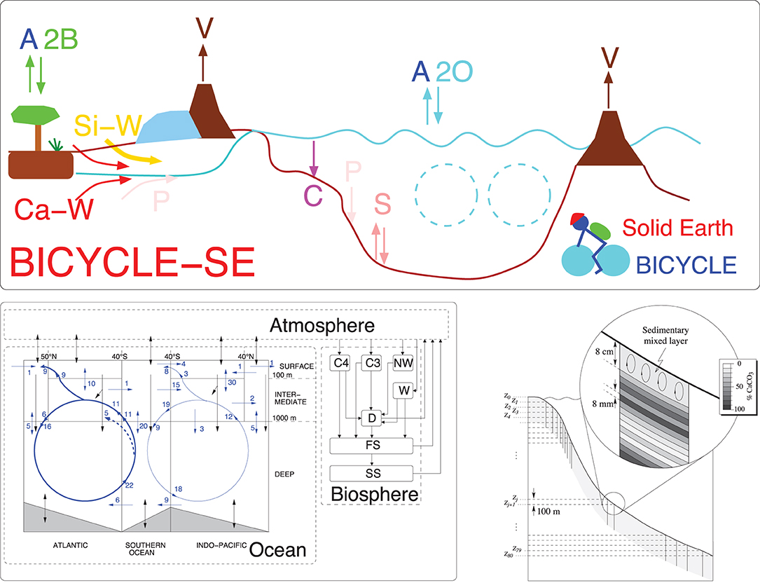
Figure 1. Sketch of the BICYCLE model. Top: Model version including solid Earth fluxes (BICYCLE-SE) explained in detail in Köhler and Munhoven (2020). V: Outgassing of CO2 from volcanoes on land potentially and temporally overlain by land ice and from hot spot island volcanoes (and mid ocean ridges, not shown) on paleo-time scales influenced by a changing sea level, but kept constant for the future scenarios investigated here; C: shallow water carbonate deposition due to coral reef growth; Si-W: silicate weathering; and Ca-W: carbonate weathering with different sources of C, but both delivering -ions into the ocean; P: riverine input and sedimentary burial; S: CaCO3 sedimentation and dissolution. A2B: atmosphere-biosphere exchange of CO2; A2O: atmosphere-ocean exchange of CO2. The cyan-colored broken circles mimic the two overturning cell in the Atlantic and Indo-Pacific Ocean. The model versions without solid Earth processes have been restricted to the fluxes A2O, A2B, and some simplified representation of carbonate compensation between ocean and sediment. Bottom left: Details of subsystem AOB (adopted from Köhler et al., 2010a) with the fixed prescribed pre-industrial water fluxes in the ocean (blue, numbers given in Sv). Black arrows denote carbon fluxes. Boxes in the land biosphere: C4, C4 ground vegetation; C3, C3 ground vegetation; NW, non-woody parts of trees; W, woody parts of trees; D, detritus; FS, fast decomposing soil; SS, slow decomposing soil. Bottom right: A conceptual sketch of the sediment module, the figure is taken from Munhoven (1997).
The model has now been extended to cover solid Earth (SE) processes Köhler and Munhoven (2020), in detail volcanic CO2 outgassing, the riverine input of from silicate and carbonate weathering, the CaCO3 sink of coral reef growth, and deep ocean CaCO3 accumulation and dissolution. Briefly, a newly implemented process-based sediment model captures early diagenesis in an 8 cm sedimentary mixed layer, under which numerous historical layers are implemented, from which CaCO3 might dissolve once the sedimentary mixed layer is thinned out. In each of the three ocean basins (Atlantic, Southern Ocean, and Indo-Pacific), the pressure-dependent carbonate system is calculated for every 100 m water depth and depending on the over- or undersaturation of the -ion, CaCO3 is either accumulated or dissolved. Implementation and realization of the sedimentary processes directly follows Munhoven and François (1996) and Munhoven (1997). Results with the simplified sedimentary response function and with the new full process-based sediment are in reasonable agreement [see Köhler and Munhoven (2020)], but for such massive perturbations as the proposed anthropogenic emissions both differ in detail, as will be discussed here. Volcanic CO2 outgassing for PI conditions and the future is kept constant at 9 · 1012 mol C/yr. Hard shells in coral reefs grow as function of sea level and Ω, the saturation state of CaCO3 (Munhoven and François, 1996) leading to a sink of carbonate of ~ 4 · 1012 mol/yr in PI times. Riverine input of silicate and carbonate weathering, partly consuming atmospheric CO2, are first kept constant at 12 · 1012 mol/yr each. However, CO2-dependent weathering (W) fluxes WX are alternatively implemented as described in Zeebe (2012), with , nSi = 0.2, and nCa = 0.4, W0 the CO2 independent weathering fluxes mentioned above, and CO2,0 the PI CO2 concentration. This approach leads to a rise in silicate (carbonate) weathering by 50% (130%) for CO2 being 8 × CO2,0 (= 2,224 ppm) reached here. These model setups are labeled AOSEW and AOSE for the new model including process-based sediments with and without CO2-dependent weathering, respectively.
In the following, results with four main setups will be discussed: the setup AOSEW and AOSE, which have been explained in the previous paragraph, in which the atmosphere–ocean is coupled to SE processes. Furthermore, I also use, for an understanding of the role of the sediments, the previous setups consisting of atmosphere–ocean with simplified (label AOS) and without (label AO) sediment feedback. The latter two setups correspond to model version 2.2 as applied in Köhler et al. (2010a) on the late Pleistocene and to some different CDR experiments with focus on C isotopes (Köhler, 2016). None of the labels include “B” (biosphere), since previous experiments (Köhler et al., 2015) have shown that the terrestrial biosphere is too simplistic to simulate meaningful results for a high CO2 world. BICYCLE's results largely differ from more complex vegetation models, probably due to an unrealistically high CO2 fertilization effect. I therefore apply the model here with a terrestrial biosphere that stays constant at PI level.
The model calculates only changes in the carbon cycle as response to changing climatic boundary conditions; it thus does not contain the physical part of the climate system. For the future emission scenarios considered here, only changes in temperature as consequence of changing atmospheric CO2 are implemented, all other environmental conditions stay constant at their pre-industrial values.
The radiative forcing of changes in CO2 on temperature is calculated as follows: The global temperature change ΔT (relevant for the atmosphere–ocean gas exchange) connected with a change in atmospheric CO2 is calculated using the transient climate sensitivity (TCS) for CO2 doubling, which has been obtained from more sophisticated climate models, and which has been recalculated to TCS = 2 K by a data-based approach (Storelvmo et al., 2016). In detail, I calculate
with
(Myhre et al., 1998). Changes in sea surface temperature (SST) are assumed to instantaneously follow ΔT, and changing SST then influences the CO2 solubility in the ocean via Henry's law.
Heat penetration into the deep ocean is not simulated, but implicitly considered by calculating surface temperature changes out of a relatively small TCS, and not out of the larger equilibrium climate sensitivity (ECS). Thus, deep ocean temperature stays constant. However, tests have shown that deep ocean temperature is not important for the simulated atmospheric CO2 concentration. Furthermore, this approach implicates that TCS, TCR (ΔT at time of 2 × CO2 in a +1%/yr CO2 rise scenario), and ECS (long-term ΔT due to 2 × CO2) are identical. This implies that CO2 and temperature change simultaneously, and the effect of a delayed warming for earlier emissions, as typically seen in GCMs, is not shown. For example, in the GISS-GCM only 60% of a CO2-induced warming is realized in the first century, and about 90% after one millennia (Hansen et al., 2011). I acknowledge that this is a bold simplification, but I will discuss how the TCR to cumulative emissions (TCRE) is compared with output from CMIP5 model for the twenty-first century. The simulated temperature change is thus comparable with GCMs on a century-time scale but underestimates warming by up to a factor of two on longer time scales.
2.2. Simulation Scenarios: High CO2 Emissions and Ocean Alkalinization
The model is spun up for 5000 years. Since PI in Keller et al. (2018) is defined as 1850 CE (100 BP), this implies that the spin ups start at 3150 BCE (5100 BP). Plotted results include only the last 100 years of the spinup, so starting at 1750 CE.
Simulations within the proposed CDR-ocean-alk experiment (including the spin up) are performed in emission driven mode, thus not prescribed CO2, but model-internal calculated atmospheric CO2 will be given in the following, circumventing slight disagreements between CO2 at PI in different sources [CDRMIP protocol (284.7 ppm in Keller et al., 2018), the CMIP6 suggested value (284.3 ppm in Meinshausen et al., 2017), and the spline through the CO2 data (286.1 ppm in Köhler et al., 2017)].
The applied fossil fuel emissions follow an extension of the Shared Socioeconomic Pathway (SSP) SSP5-85-EXT++ (Riahi et al., 2017). Since long-term emissions have not been available in 2018, when simulations have been performed, they have been compiled as follows. CO2 emissions for SSP5-85-EXT should agree with Figure 5 in O'Neill et al. (2016). My CO2 historical emissions (fossil fuel (+ industry) and land use change) until 2005 CE are as compiled for RCP8.5 in Meinshausen et al. (2011). For 2006–2100 CE fossil fuel (+ industry), CO2 emissions are taken from https://esgf-node.llnl.gov/projects/input4mips/ as prescribed for CMIP6 (Hoesly et al., 2018), but CO2 emissions from land use change (2006–2015 CE) is used as published in Houghton and Nassikas (2017), one of two bookkeeping models in Le Quéré et al. (2018). The extension of the emissions for years 2100–2300 CE is built from scratch following the description in O'Neill et al. (2016). Note that 2250–2300 CE should have emissions “of just below 10 PgC/yr.” Here, I take 9.5 PgC/yr. Following a discussion with the coordinator of CDRMIP (Keller, personal communication), emissions are extended from 2300 CE with a linear reduction reaching zero emissions in year 2350 CE and stay zero thereafter. The simulations are extended by at least 5000 years (and up to ~1 million years) in the future. The annual emissions peak in year 2090 CE at 35.6 PgC/yr and the total cumulative CO2 emissions of this scenario add up to 6740 PgC (Figure 2A). This emission scenario SSP5-85-EXT++ without alkalinization is my control run (CTRL).
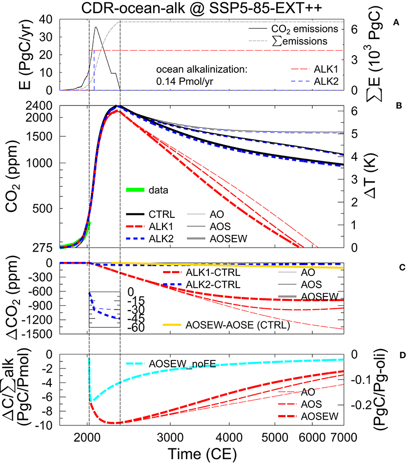
Figure 2. (A) CO2 emissions of the control run SSP5-85-EXT++ (annual and cumulative emissions E and left and right y-axis, respectively). Timing of ocean alkalinization of 0.14 Pmol/yr in scenarios ALK1 and ALK2 sketched in red and blues lines, respectively (no y-axis). (B) Resulting atmospheric CO2 (left y-axis on log scale) and global temperature change ΔT with respect to pre-industrial (right y-axis) including a spline through compiled CO2 data (Köhler et al., 2017), extending years 2016–2019 CE with online available data from NOAA. (C) Anomaly in atmospheric CO2 with respect to a CTRL with alkalinization in scenarios ALK1 and ALK2. Zoom-in shows otherwise hardly detectable changes in atmospheric CO2 due to ALK2 (results for AO and AOS are not distinguishable). Additionally the contribution of the CO2-dependent weathering in the CTRL runs is shown. (D) Efficiency of ocean alkalinization (ratio of C extracted from the atmosphere over accumulated alkalinization) in ALK1. On the right y-axis, the efficiency is transferred in PgC/Pg of olivine assuming a molar mass of 140 g/mol corresponding to the iron-free version of olivine called forsterite (Mg2SiO4). Additionally, efficiency is shown for a scenario without future emissions (AOSEW_noFE). In (B,C,D), results from three different setups are plotted: atmosphere-ocean only (AO), atmosphere-ocean including a sedimentary response function (AOS), or atmosphere-ocean in a solid Earth setup including CO2-dependent weathering (AOSEW), having the terrestrial biosphere always fixed at pre-industrial levels. Vertical lines are at 2020 CE (onset of alkalinization) and 2350 CE (emissions back to 0). Note, that the x-axes are on log scale.
In addition to the CTRL, two different ocean alkalinization scenarios are applied. In ALK1 0.14 Pmol/yr, alkalinity is put into the surface ocean from year 2020 CE onward until the end of the simulation in year 7020 CE. From this alkalinization, 50% is put in each of the two 100 m deep equatorial surface ocean boxes ranging from 40°S to 50°N in the Atlantic and to 40°N in the Pacific. This approach follows the CDRMIP protocol putting the alkalinization in surface waters free of sea ice. Furthermore, it has been shown that a large amount of material, which needs to dissolve for such an alkalinity input, might due to the temperature-dependent kinetics sink undissolved into the abyss, when applied in polar waters (Köhler et al., 2013). In ALK2, this alkalinity input stops after 50 years in 2070 CE. Adding 0.14 Pmol/yr alkalinity is equivalent to adding 5.19 Pg/yr of an alkalizing agent like Ca(OH)2 or 4.92 Pg/yr of forsterite (Mg2SiO4), a form of olivine. When assuming a theoretically possible net instant dissolution reaction, every mole of the added Ca(OH)2 or Mg2SiO4 would sequester 2 or 4 mol of CO2, respectively (Ilyina et al., 2013; Köhler et al., 2013). However, this back-of-the-envelope approximation ignores changes in sequestration efficiency due to the non-linear marine carbonate chemistry response as will be discussed in detail in the Results section.
These three scenarios (CTRL, ALK1, ALK2) are simulated in the different model setups described in section 2.1. An overview of all scenarios and setups used here is compiled in Table 1.
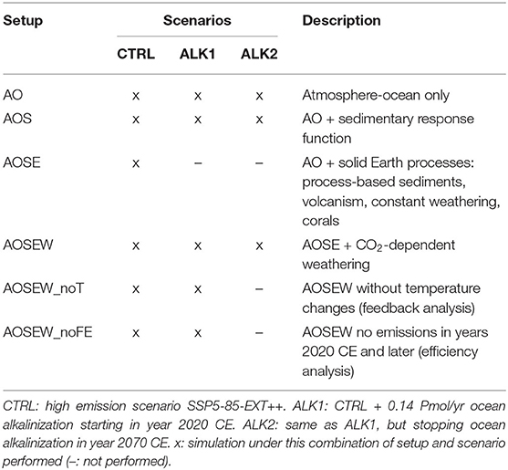
Table 1. Compilation of simulated scenarios and setups.
3. Results
Simulated CO2 depends on the specific setup and varies between 261 and 276 ppm in year 1750 CE, rising to 437–456 ppm in year 2019 CE, thus faster than the historical reconstructed rise from 277 to 410 ppm in the same time window (Figure 2B). This difference in the historical CO2 evolution can be understood by the missing terrestrial carbon sink, which nowadays sequestrates about one-fourth to one-third of the anthropogenic emissions (Friedlingstein et al., 2019).
In all investigated scenarios, the anthropogenic CO2 emissions in the twenty-first century largely dominate the global carbon cycle. Initial differences of the carbon cycle in the different model versions after spin-up are quickly dwarfed by the proposed emissions in the SSP5-85-EXT++ scenario, which is more than triple from the present-day (2020) fluxes of ~10 PgC/yr within the next 70 years. Atmospheric CO2 concentration peaks nearly independently of model version with 2,400 ppm in years 2326, only 24 years before the final fade out of any fossil fuel emissions. If alkalinization is applied (ALK1), the CO2 peak is smaller by 200 ppm than without those sequestration efforts (Figure 2B).
While the long-term evolution of CO2 in the CTRL runs largely depend on the sediment and weathering feedbacks, having values in year 7000 between 965 and 1,600 ppm, the resulting atmospheric CO2 during sustained alkalinization (ALK1) obtained with different model versions is more in agreement. Here, atmospheric CO2 falls below its pre-industrial value—implying the complete neutralization of all anthropogenic emissions—between the years 5500 and 6100.
The long-term atmospheric CO2 in the control simulations depends on the setup (Figure 2B), since in AO only the oceanic carbon uptake is reducing CO2, while in AOS the carbonate compensation mimicking the dissolution of CaCO3 allows a further CO2 reduction. Furthermore, in AOSEW a different CaCO3 dissolution scheme together with a small contribution of <110 ppm from CO2-dependent enhanced weathering fluxes (Figure 2C) reduces CO2 to even lower levels. Simulated atmospheric CO2 in the alkalinization experiment ALK1 is more setup independent than for the CTRL runs (Figure 2B). This implies that the details of CO2 sequestration largely differ in the different setup (Figure 2C), for example, varying from sequestrated 800 ppm in AOSEW to 1,400 ppm in AO. It also shows that the CO2 sequestration potential for high emission scenarios obtained with carbon cycle models without sediment modules is overestimated after roughly a millennium. However, already on multi-centennial time scales the simulated marine carbonate chemistry (e.g., pH, ocean alkalinity, Figure 3) is influenced by the dissolution of sediments, a process which is missing in setups without sediment/ocean interaction.

Figure 3. (A) Volume-weighted mean pH of all surface ocean boxes. (B) C content of atmosphere (A) and ocean (O), marking the additional C released from the dissolution of CaCO3 in the sediments due to the carbonate compensation feedback. Legend in (A) is also used in (B). (C) Total alkalinity for different CTRL runs. (D) Changes in total alkalinity for ALK1 in different setups. Vertical lines are at 2020 CE (onset of alkalinization) and 2350 CE (emissions back to 0). Note log x-axis. Units of Eg or Emol correspond to 1018 g or mol.
Coral reef growth (included in AOSEW) is a sink for alkalinity and a source of CO2. However, the impact of its variability on the carbon cycle is negligible. In both CTRL and ALK1, the reef growth declines by three orders of magnitude in the first half of the future simulation. During ocean alkalinization, Ω and a potential coral reef growth would rise again, the latter to 10 · 1012 mol/yr after 3000 years. Thus, in comparison to pre-industrial conditions, an initial CO2 gain caused by reduced coral reef growth of <20 ppm is compensated by a similarly large CO2 loss later on. However, this ignores the potential that corals get extinct due to a prolonged fall of Ω below critical values. If so their contribution as CaCO3 sink might not reach initial values again even if chemical conditions no longer dissolve their CaCO3-based skeletons.
In all setups, the efficiency of the ocean alkalinization has its maximum with 9.7 PgC oceanic carbon uptake per Pmol alkalinity input after 200 years during times of maximum anthropogenic emission, after which the efficiency slowly decreases to 2–4 PgC/Pmol (Figure 2D). These values correspond to 0.27 and 0.05–0.1 PgC per Pg of olivine, respectively, if alkalinization is realized by the dissolution of forsterite. A reduction in efficiency of 20% when increasing the amount CO2 sequestered by olivine dissolution from 1 to 20 PgC has been proposed based on calculations of the marine carbonate system, but ignoring ocean-sediment interaction and the importance of changes in the anthropogenic CO2 emissions (Köhler et al., 2010b). I therefore test the influence of the prescribed rise in anthropogenic emissions on the calculated efficiency by an additional ocean alkalinization experiment without future CO2 emissions (AOSEW_noFE). I indeed find after a 2–3 decades for equilibration (and increasing efficiency) a decrease in efficiency from its peak value of 6.5 PgC/Pmol alkalinity input, clearly different from the evolution of the sequestration efficiency that includes the proposed rise in CO2 emissions (Figure 2D). I find a larger reduction in CO2 sequestration efficiency in setups with sediments compared to AO-only setups, which is caused by a decline of the artificially added alkalinity (or its residence time) in the ocean (Figure 3D). In detail, on the long run the additional alkalinity leads to a deepening of the calcite saturation horizons (CSHs) and the lysocline transition zones (Figure 4), and finally to a rise of CaCO3 accumulation in the sediments, which extracts alkalinity from the ocean and thus reduces the carbon sequestration efficiency.
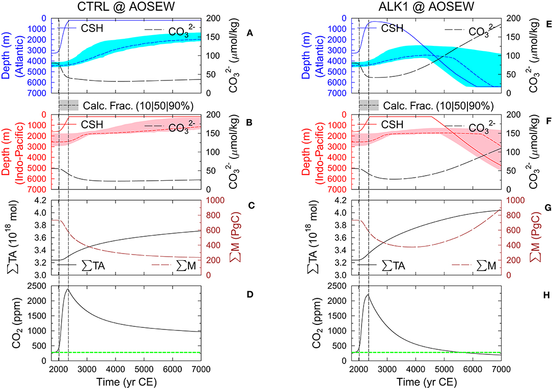
Figure 4. Details for CTRL (left) and ALK1 (right) in AOSEW setup. Calcite saturation depth (CSH), carbonate fraction (shaded area covers depths from 10% (lower bound) to 90% (upper bound) with 50% as short broken line in-between) in sedimentary mixed layers, and -ion concentration in the equatorial ocean of the (A,E) Atlantic or (B,F) Indo-Pacific. (C,G) Sum of total alkalinity in the ocean (∑TA) and global amount of CaCO3 integrated over all sedimentary mixed layer (∑M). (D,H) Atmospheric CO2, and green horizontal line marks the pre-industrial concentration of 278 ppm. Vertical lines are at 2020 CE (onset of alkalinization) and 2350 CE (emissions back to 0).
In the scenario ALK2 containing 50 years of alkalinization, only a very small amount of carbon is sequestered (Figures 2A–C). Following back-of-the-envelope calculations for olivine (Köhler et al., 2010b), in this scenario about 250 Pg of olivine should lead to a reduction in CO2 of ~30 ppm, a difference that is indeed realized around the CO2 peak in the 2320s years, but then contributes only to a relative reduction in CO2 of 1–2%. However, after several thousand years the long-term sequestration in ALK2 is reduced to 10–20 ppm in setups with sediment feedback. This long-term change in CO2 sequestration shows that ocean alkalinization is not a permanent artificial CO2 sink, but depends in detail on how alkalinity is preserved in the ocean.
Surface ocean pH is back to its pre-industrial values of 8.1–8.2 between years 5000 and 6000 in ALK1 and results agree between different model setups similarly as when all anthropogenic emissions have been neutralized (Figure 3A). The pH minima of ~7.3–7.4 mirror the peaks in atmospheric CO2. pH in CTRL and ALK2 are similarly setup dependent as atmospheric CO2.
The effect of the sediment feedback is easily illustrated, when plotting the sum of carbon contained in both the atmosphere and the ocean (Figure 3B). While in setups without sediments this number can only increase due to anthropogenic emissions, it might additionally be modified by the dissolution or accumulation of CaCO3 in the sediments. In the SE setup (AOSEW), some small contributions from volcanic CO2 outgassing, CO2-dependent weathering, and shallow water deposition of CaCO3 in corals might also play a role, but these fluxes are on the order of <30 Tmol/yr each, and over the simulated 5000 years about two orders of magnitude smaller than the cumulative CO2 emission, and therefore negligible. However, what mainly happens in setups with interactive sediments is CaCO3 dissolution (colored areas in Figure 3B), which is reduced when ocean alkalinization is applied. The artificial input of alkalinity does not prevent the CaCO3 dissolution in sediments. In my modeling approach, about 2.3 EgC are dissolved from the sediments in CTRL, and nearly half of it during the first 1000 years after the end of the anthropogenic emissions. This dissolution during the first millennium hardly changes during ocean alkalinization. However, later on CaCO3 accumulation in the sediment is again possible, having in year 7000 CE again a nearly similar amount of carbon in the combined ocean–atmosphere system as at the end of the emissions. The amount of dissolvable CaCO3 depends on the initial sedimentary inventory, which has been generated after 800 kyr of simulations. The 8 cm thick sedimentary mixed layer contains globally integrated ~ 700 PgC, but there are up to 500 historical sediment layers of 8 mm each underneath, which might also dissolved, once the sedimentary mixed layer is sufficiently thinned out. Similar as other parts of the model, the process-based sediment module is simpler than in full GCMs leading to larger dissolvable CaCO3 than in other studies. For example, Archer et al. (1998) suggest that only 1.6 EgC of sedimentary CaCO3 can be dissolved. This implies that the neutralization of anthropogenic emissions by sediment dissolution—the sediment feedback—might be slightly overestimated in this study.
A closer look on the sediment–ocean interaction gives the following details: In the water column, the rise in the CSH close to the ocean surface accompanied by a drop in -ion concentration is clearly seen in the Atlantic and the Indo-Pacific for both CTRL and ALK1 (Figures 4A–F). Note that for technical reasons related to the implementation of sea level change in BICYCLE, the CSH cannot rise above 200 m water depth. The sedimentary response to this vertical rise in the CSH is by several thousands of years delayed and follows as an upward shift of the lysocline transient zone of partially dissolved sediments (Figures 4A,B), implying especially a dissolution of CaCO3 from the sediments in water depths in which this transition zone has moved to a shallower depth. The amount of CaCO3 in the sedimentary mixed layer gradually declines in CTRL from 700 to slightly more than 200 PgC (Figure 4C). The fact that this number has not been reduced to zero indicates that after 5000 simulated years historical layers are still included into the sedimentary mixed layer and then also potentially dissolved. This process slows down over time due to the increasing fraction of non-CaCO3 material (clay), which is on the long run included in the sedimentary mixed layer, effectively limiting the amount of dissolved CaCO3 (e.g., see also Archer et al., 1998). Ocean alkalinization is able to reverse these trends bringing CSH and -ion concentration back to initial values and even beyond if alkalinity input is sustained until the end of the simulation time (Figures 4E,F). The water depth in which the lysocline transition zone is found deepens and widens having in the end a several kilometer deep band in which the fraction of CaCO3 in the sedimentary mixed layer decreases from 90% (upper bound) to 10% (lower bound). Especially the lower bound is found in deeper waters than before, indicating that ocean alkalinization would allow CaCO3 accumulation in the sediments at water depths at which in pre-industrial times a complete dissolution of CaCO3 would have occurred (Figures 4E,F). In ALK1, the total amount of CaCO3 in the sedimentary mixed layer increases again after passing its minimum of 400 PgC around year 4000 CE (Figure 4G).
The total alkalinity in the ocean is, similarly as the total amount of carbon in the AO subsystem, depending on the consideration of the sediment feedback (Figure 3C), since, as already explained, the anthropogenic carbon penetrating the deep ocean partly dissolves the sediment. Therefore, the alkalinization experiments change alkalinity differently (Figure 3D): in setups with interactive sediments, further alkalinity input changes the deep ocean–sediment exchange fluxes due to vertical shifts in the CSH toward deeper water, allowing later in the simulation an increase in sedimentary CaCO3 accumulation. The loss of CaCO3 from the ocean to the sediment is a sink for oceanic alkalinity, therefore reducing total alkalinity in comparison to setups without sedimentary responses (AO).
The strength of the temperature, sediment, and weathering feedbacks can be approximated by plotting differences obtained with setups with the relevant processes being switched on or off (Figure 5). I obtained the strength of the feedbacks by calculating differences from the same standard runs obtained with the setup AOSEW. In detail, the temperature feedback is based on ΔT = AOSEW – AOSEW_noT, in which the latter is a special case in which temperature is kept constant; the weathering feedback is derived from ΔW = AOSEW – AOSE; the sediment feedback from ΔS = AOSEW – AO – ΔW. I find that the positive temperature feedback adds about 150 ppm of CO2 to the atmosphere, which also persists for several millennia. In other words, carbon cycles with and without temperature feedback do not instantaneously agree with each other once the anthropogenic emissions drop back to zero, since the changes in CO2 solubility introduced by temperature have in the mean time penetrated into the deep ocean. The negative feedbacks reduce CO2 by 520 (sediment) and 110 (weathering) ppm over the next 5000 years in the CTRL run. In ALK1, all feedbacks are back to zero after 5000 years, since all anthropogenic emissions have been sequestrated after 3500–4100 years, and existing carbon cycle realizations were slowly merging toward each other, thus marginalizing any differences. Assuming a higher climate sensitivity, for example, more in agreement with its values for equilibrium conditions of 2.6–3.9 K (the 66% probability range in the most recent review of Sherwood et al., 2020) would lead to higher CO2 concentrations of 30–100 ppm and therefore to a higher temperature feedback. Such higher numbers are probably expectable in the long run (millennium scale), but should be an overestimation for the next centuries, since the full climate response to CO2 takes 1–2 kyrs (Hansen et al., 2011).
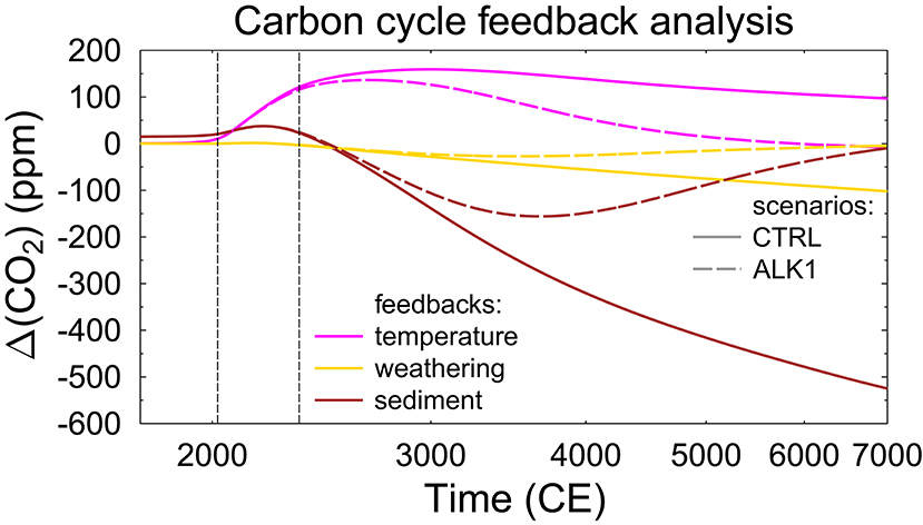
Figure 5. Feedback analysis of the contribution of the positive temperature feedback, and the negative weathering and sediment feedback on the CTRL run and alkalinization scenario ALK1. Vertical lines are at 2020 CE (onset of alkalinization) and 2350 CE (emissions back to 0). Note log x-axis.
The strength of the feedbacks in the CTRL simulations without alkalinization is comparable to feedbacks in other models. For example, CO2 anomalies after 10 kyr in a 5000 PgC carbon pulse experiment have been +50 to +400 ppm (climate), −70 to −220 ppm (weathering), and −200 to −550 ppm (sediment) in the in the Long-Term MIP with 5–7 more complex climate models (Archer et al., 2009). The vegetation feedback neglected here is usually a negative feedback reducing CO2 even further. However, the strength of this feedback is typically reduced over time, potentially also switching to a positive feedback. Paleo studies (Retallack and Conde, 2020) indicate that atmospheric CO2 concentrations above 1,500 ppm might be toxic to the biosphere, making the vegetation response in a high CO2 world a rather unknown variable. Furthermore, in Long-Term MIP a climate feedback, not a temperature feedback, is calculated, since in applied models any change in the radiative forcing does not only change temperature as in my box model here, but also other climatic processes. Most importantly for the carbon cycle—and missing here—is a potential reduction or even shutdown of the Atlantic meridional ocean circulation (e.g., Liu et al., 2017), since this would alter the transport of tracers between the surface and the deep ocean, and thus alter the marine carbon pumps. Additionally, permafrost thaw in a high emission world will most likely lead to additional CO2 (and CH4) fluxes to the atmosphere not accounted for here and in most other models (e.g., Burke et al., 2018).
The temporal response of the carbon cycle to the anthropogenic emissions is often analyzed as the “airborne fraction” f = ΔCA/∑E, which describes the ratio of the difference in atmospheric carbon content ΔCA over cumulative emissions ∑E (Figure 6). Once f is brought back to zero, all anthropogenic emissions have been extracted from the atmosphere and CO2 has reached pre-industrial concentration again. This fraction reaches 0.7 during peak emission times and is gradually reduced depending on implemented processes. Without interactive sediments it stays above 0.4. The sediment feedback reduces f to 0.1 after 20–40 kyr. Interestingly, both setup with simplified sedimentary response function and process-based sediment reach nearly identical end points, but differ only on their ways toward them. Here, the effect of the response function (AOS) is slower than the process-based sediment (AOSE) until year 9000, while the response function reduces atmospheric CO2 faster thereafter. This implies that at first sediment dissolution might occur faster than approximated with the response function, while later on this process is slowed down, probably due to the limited amount of available CaCO3, which can be dissolved. The weathering feedback reduces CO2 during the whole simulation time, but was especially necessary to gradually bring the airborne fraction from 0.1 down to zero (atmospheric CO2 back to pre-industrial values) on a million years time scale, in agreement with others (e.g., Colbourn et al., 2013). The effect of the alkalinization is an acceleration of the reduction of f toward zero. Airborne fractions f discussed above differ from the numbers given in the introduction due to the difference in the amount and temporal evolution of the anthropogenic emissions.
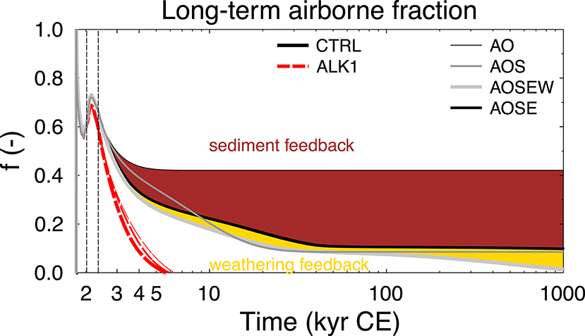
Figure 6. Airborne fraction f of anthropogenic emissions for different model versions for up to 1,000 kyr CE (=1 Myr CE) in the CTRL run and alkalinization scenario ALK1. The color-coded areas show the CO2 sequestration related to weathering and sediment feedback. Vertical lines are at 2020 CE (onset of alkalinization) and 2350 CE (emissions back to 0). Note log x-axis.
4. Discussion
In the following discussion I will first (section 4.1) focus on the general model response including an analytical view on the TCR to cumulative emissions (TCRE) to obtain an in-depth understanding of the underlying emission scenarios. TCREs is not central to the ocean alkalinization experiments but gives an understanding for the consequences of the implemented climate sensitivity in the model and sets the box model results in relation to more complex approaches. In the second part, I will then discuss the alkalinization experiments (section 4.2).
4.1. General Model Response to Anthropogenic Emissions Including TCRE
Although the BICYCLE model is focusing on the carbon cycle and has only a very limited implementation of climate change, it is useful to compare the resulting temperature change with output of more complex models. For this effort, TCRE is plotted together with previous simulations of RCP emission scenarios (Köhler, 2016) and CMIP5 contributions (Figure 7).
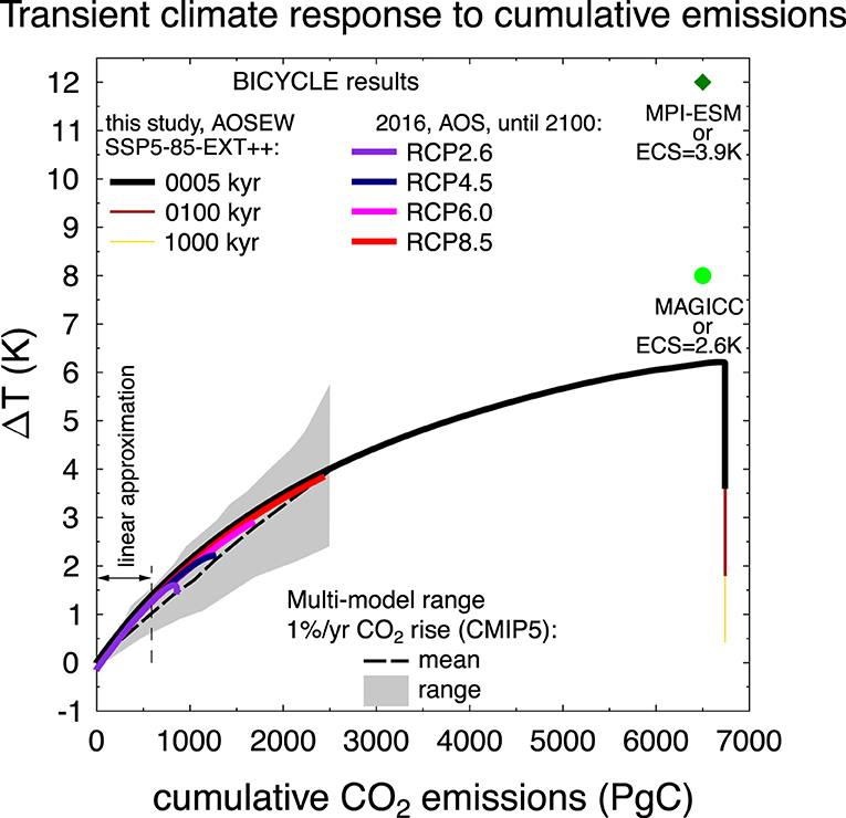
Figure 7. Global mean surface temperature increase as a function of cumulative net global CO2 emissions, known as transient climate response to cumulative emissions (TCRE) for results from BICYCLE and other models. From this study, results for CTRL (emissions following scenario SSP5-85-EXT++) in model version AOSEW for 5, 100, and 1,000 kyr are shown. In addition, four different RCP emission scenarios (BICYCLE, model version AOS) from Köhler (2016) are included. The 2016 results show changes from the beginning of the emissions (year 1765) until year 2100. For the BICYCLE results I directly calculate ΔT from CO2 using a transient climate response of 2 K as given in the methods. For comparison the multi-model mean and range simulated by CMIP5 models, forced by a CO2 increase of 1% per year is given by the broken black line and gray area (after Figure SPM 10 of IPCC, 2013). These simulations exhibit lower warming than those driven by RCPs within CMIP5, which include additional non-CO2 forcing and therefore lead to higher temperature changes. For the CMIP5 results, ΔT until the year 2100 is calculated relative to the 1861–1880, and CO2 emissions relative to 1870. I also included the discussed warmings obtained with an ECS of 2.6 or 3.9 K, identical to the simulations for SSP5-85-EXT CO2 emissions (6500 PgC) obtained with the simple climate model MAGICC (O'Neill et al., 2016) and MPI-ESM (Kleinen, personal communication). The range with cumulative emissions <590 PgC approximated by a linear relationship in the TCRE in the analysis is also marked.
CMIP5 results (IPCC, 2013) are here restricted to idealized scenarios with CO2 emissions only, in detail to those with 1%/yr rise in CO2. This approach neglects global warming connected with anthropogenic emissions of CH4, N2O, or any aerosol effects, which are also ignored in BICYCLE, and thus allowing a meaningful comparison. For cumulative emissions of 2,500 Pg C, the spread in the simulated global warming ΔT in the CMIP5 output ranges from 2.2 to 5.5 K. BICYCLE results are very well in the middle of the uncertainty range spanned by simulation results of the Earth system models (ESM) contributing to CMIP5, but show especially for higher cumulative emissions a clear non-linear relationship between ΔT and ∑E, the so-called TCRE. The drop in ΔT from >6 K to <0.5 K for constant ∑E in our SSP5-85-EXT++ simulation reflects the sequestration of anthropogenic CO2 first by marine uptake, followed by the sediment and the weathering feedbacks.
More complex models find a near linear trend for TCRE (e.g., Allen et al., 2009; Goodwin et al., 2015; Frölicher, 2016; MacDougall, 2016, 2017; Tokarska et al., 2016; Seshadri, 2017; Williams et al., 2017; Katavouta et al., 2018; Rogelj et al., 2019). This relationship compresses the anthropogenic impact on climate into one relationship and one figure, which make the man-made global warming rather easy to grasp and to communicate. Therefore, such a figure has also been included in the last assessment report of the IPCC [Figure 10 in the Summary for Policy Makers (IPCC, 2013)]. Here, I will elaborate why simulation results with a carbon cycle box model also show this behavior by analytically analyzing why and when the ratio of global temperature change over cumulative net CO2 emissions should be constant.
The relation between CO2 and ΔT in BICYCLE has already been described in the methods section with Equations (1) and (2) for ΔT = f(ΔRCO2) and ΔRCO2 = f(CO2), respectively.
The CO2-dependent term in the natural logarithmic function in Equation (2) can be rewritten as
with CA: CO2 content in the atmosphere, : baseline CO2 content in the atmosphere (278 ppm or 589 PgC using the well-known correlation of 1 ppm = 2.12 PgC), ΔCA: the change in atmospheric CO2 from the baseline. Using as approximation the first term of the Taylor series for the natural logarithmic
which converges for x ∈ (−1, +1] (or here for ΔCA ≤ 589 PgC) I find
Neglecting changes in the terrestrial carbon storage (as done in those simulations with BICYCLE), the cumulative net emissions, ∑E, can be expressed as follows:
with ΔCO: the oceanic uptake of anthropogenic CO2 emissions. Using
with f being the airborne fraction. The net emissions can also be expressed as
Following our analysis above (Equations 7 and 12), the relationship between global surface temperature change, ΔT, and the cumulative net emissions, ∑E, can be expressed as
which is for ∑E < 590 PgC to the first order a linear relation (constant slope), since f ~ 0.6 and changes only very little during the first centuries of the anthropogenic emissions.
Thus, TCRE, is a function of the airborne fraction. In our model results, they are roughly pathway independent until the mid-21st century, when they start to diverge (see Köhler, 2016). This implies that TCRE is not completely pathway independent but depends on the airborne fraction, which depends on the anthropogenic emission strength (e.g., Joos et al., 2013; Lord et al., 2016).
The non-linear character of the TCRE relationship in our results, especially for ∑E > 589 PgC, is directly obtained, if the approximation of Equation (7) with the Taylor series is not performed, or if a longer simulation time is analyzed, in which f gradually declines toward lower values. The equations for an explanation of TCRE become more complicated if the oceanic heat uptake is not considered implicitly via TCR, but explicitly (MacDougall, 2017). Models, which have ocean heat uptake implemented, typically also calculate proposed changes in ocean circulation and subsequent oceanic CO2 uptake. They obtain for high cumulative emissions larger temperatures than the box model used here, and are thus more in line with a linear relationship in TCRE generally found for complex climate models. The long-term temperature response can be approximated if I assume an ECS of 2.6–3.9 according to Sherwood et al. (2020) instead of the TCR of 2 K used here. This would lead to a long-term ΔT for the full cumulative emissions of 8–12 K (instead of ~6 K seen in Figure 7), more in agreement with SSP5-85-EXT-based warming of 8 K obtained with the simple climate model MAGICC (O'Neill et al., 2016) or of 12 K simulated with the MPI-ESM (Kleinen, personal communication).
4.2. Alkalinization
The performed alkalinization in CDR-ocean-alk leaves the question open which mineral should be dissolved to reduce CO2. It is therefore also not possible to address if and how marine biology might be largely altered, since it is not clear which nutrients, in addition to alkalinity, might be added to the ocean. In a simulation experiment in which the dissolution of olivine has been implemented (Hauck et al., 2016) large shifts in the phytoplankton community due to silicic acid and iron input accompanying the olivine dissolution have been found. In experiments, in which 1-mol-% of the olivine contains bioavailable iron, the relative contributions to the total CO2 sequestration by olivine dissolution have been 57% via alkalinity input, 37% via iron fertilization, and 6% via silicic acid input. The part of the CDR caused by ocean fertilization (iron, silicic acid) is not permanent, while the CO2 sequestered by alkalinization would be stored in the ocean as long as alkalinity is not removed from the system (Hauck et al., 2016).
The amount of material necessary for a complete sequestration of all anthropogenic emissions is huge. An atmospheric CO2 concentration of 400, 350, 300, or even 280 ppm is reached only after 2730, 3060, 3480, or 3710 years of a constant alkalinization of 0.14 Pmol/yr, respectively. If olivine is used for this effort, 13.4–18.2 Eg of this silicate rock needs to be mined, grinded, and transported to suitable places, preferable to tropical waters that allow fast mineral dissolution (Köhler et al., 2013). For any application of ocean alkalinization, its sequestration efficiency maximum around peak CO2 emissions needs to be considered. The time spans until complete neutralization are difficult to grasp, since they contain more than 100 generations of mankind. It clearly illustrates that, if this process might help for CO2 sequestration, it certainly is not enough to rely on only ocean alkalinization of the suggested magnitude. It needs more efforts to bring atmospheric CO2 down faster. Preferably, the high emission world underlying our simulations here is not the one mankind has to deal with. However future emissions might look like most likely a suite of different approaches is needed to fully counteract the amplitude of the anthropogenic emissions. For example, they might follow a multi-wedge approach, in which various different mechanisms are simultaneously applied for an efficient and manageable neutralization of anthropogenic CO2 emissions in the foreseeable future (Pacala and Socolow, 2004; Davis et al., 2013).
5. Conclusions
I here described long-term effects of ocean alkalinization in a high emission world using a simple carbon cycle box model with fixed marine and terrestrial biology and unchanged ocean circulation. The assumed cumulative CO2 emissions of 6,740 PgC would by oceanic processes and sediment and weathering feedbacks be naturally extracted from the atmosphere on time scales of 105 − 106 years. Ocean alkalinization of the proposed strength—equal to an annually constant dissolution of 5 Pg of olivine—would shorten this neutralization time of anthropogenic emissions to ~3500 years. The carbon sequestration efficiency of ocean alkalinization has its maximum during the anthropogenic CO2 emission peak and shortly thereafter at 9.7 PgC per Pmol of alkalinization (or 0.27 PgC/Pg of olivine) slowly declining to half of this value two millennia later. The alkalinization partly compensates the natural occurring fossil fuel neutralization by CaCO3 dissolution from ocean sediments. The thus altered marine chemistry reverses after 1–2 kyr the trend from sedimentary CaCO3 dissolution to a restrengthened accumulation of CaCO3 in the sediments. Ocean alkalinization extracts anthropogenic CO2 from the atmosphere only as long as the added alkalinity stays in the ocean, which can due to ongoing CaCO3 accumulation in the sediments not be guaranteed for 100% of the artificially added alkalinity.
Data Availability Statement
The datasets generated and analyzed for this study can be found in the PANGAEA data base (https://doi.org/10.1594/PANGAEA.921107).
Author Contributions
PK was the sole developer of the applied model BICYCLE, followed the conceptional design of the CDRMIP scenario CDR-ocean-alk, performed all the simulations, analyzed the results, and wrote the paper.
Funding
PK was institutional funded by AWI via the Helmholtz research program PACES-II.
Conflict of Interest
The author declares that the research was conducted in the absence of any commercial or financial relationships that could be construed as a potential conflict of interest.
Acknowledgments
I thank Guy Munhoven for providing model code, part of Figure 1, and discussions on the sediment model over the years. I thank the coordinators of the CDRMIP for their work in getting this effort going, and Thomas Kleinen for sharing his unpublished results with me.
References
Allen, M. R., Frame, D. J., Huntingford, C., Jones, C. D., Lowe, J. A., Meinshausen, M., et al. (2009). Warming caused by cumulative carbon emissions towards the trillionth tonne. Nature 458, 1163–1166. doi: 10.1038/nature08019
Archer, D., Eby, M., Brovkin, V., Ridgwell, A., Cao, L., Mikolajewicz, U., et al. (2009). Atmospheric lifetime of fossil fuel carbon dioxide. Annu. Rev. Earth Planet. Sci. 37, 117–134. doi: 10.1146/annurev.earth.031208.100206
Archer, D., Kheshgi, H., and Maier-Reimer, E. (1997). Multiple time scales for neutralization of fossil fuel CO2. Geophys. Res. Lett. 24, 405–408. doi: 10.1029/97GL00168
Archer, D., Kheshgi, H., and Maier-Reimer, E. (1998). Dynamics of fossil fuel neutralization by marine CaCO3. Glob. Biogeochem. Cycles 12, 259–276. doi: 10.1029/98GB00744
Beerling, D. J., Kantzas, E. P., Lomas, M. R., Wade, P., Eufrasio, R. M., Renforth, P., et al. (2020). Potential for large-scale CO2 removal via enhanced rock weathering with croplands. Nature 583, 242–248. doi: 10.1038/s41586-020-2448-9
Burke, E. J., Chadburn, S. E., Huntingford, C., and Jones, C. D. (2018). CO2 loss by permafrost thawing implies additional emissions reductions to limit warming to 1.5 or 2°C. Environ. Res. Lett. 13:024024. doi: 10.1088/1748-9326/aaa138
Colbourn, G., Ridgwell, A., and Lenton, T. M. (2013). The Rock geochemical model (RokGeM) v0.9. Geosci. Model Dev. 6, 1543–1573. doi: 10.5194/gmd-6-1543-2013
Colbourn, G., Ridgwell, A., and Lenton, T. M. (2015). The time scale of the silicate weathering negative feedback on atmospheric CO2. Glob. Biogeochem. Cycles 29, 583–596. doi: 10.1002/2014GB005054
Committee on Geoengineering Climate (2015). Climate Intervention: Carbon Dioxide Removal and Reliable Sequestration. Washington, DC: National Academic Press.
Davis, S. J., Cao, L., Caldeira, K., and Hoffert, M. I. (2013). Rethinking wedges. Environ. Res. Lett. 8:011001. doi: 10.1088/1748-9326/8/1/011001
Friedlingstein, P., Jones, M. W., O'Sullivan, M., Andrew, R. M., Hauck, J., Peters, G. P., et al. (2019). Global carbon budget 2019. Earth Syst. Sci. Data 11, 1783–1838. doi: 10.5194/essd-11-1783-2019
Frölicher, T. L. (2016). Climate response: strong warming at high emissions. Nat. Clim. Change 6, 823–824. doi: 10.1038/nclimate3053
Ganachaud, A., and Wunsch, C. (2000). Improved estimates of global ocean circulation, heat transport and mixing from hydrographic data. Nature 408, 453–457. doi: 10.1038/35044048
González, M. F., and Ilyina, T. (2016). Impacts of artificial ocean alkalinization on the carbon cycle and climate in Earth system simulations. Geophys. Res. Lett. 43, 6493–6502. doi: 10.1002/2016GL068576
Goodwin, P., Williams, R. G., and Ridgwell, A. (2015). Sensitivity of climate to cumulative carbon emissions due to compensation of ocean heat and carbon uptake. Nat. Geosci. 8, 29–34. doi: 10.1038/ngeo2304
Hansen, J., Sato, M., Kharecha, P., and von Schuckmann, K. (2011). Earth's energy imbalance and implications. Atmos. Chem. Phys. 11, 13421–13449. doi: 10.5194/acp-11-13421-2011
Hauck, J., Köhler, P., Wolf-Gladrow, D. A., and Völker, C. (2016). Iron fertilisation and century-scale effects of open ocean dissolution of olivine in a simulated CO2 removal experiment. Environ. Res. Lett. 11:024007. doi: 10.1088/1748-9326/11/2/024007
Haverd, V., Smith, B., Canadell, J. G., Cuntz, M., Mikaloff-Fletcher, S., Farquhar, G., et al. (2020). Higher than expected CO2 fertilization inferred from leaf to global observations. Glob. Change Biol. 26, 2390–2402. doi: 10.1111/gcb.14950
Heimann, M., and Maier-Reimer, E. (1996). On the relations between the oceanic uptake of CO2 and its carbon isotopes. Glob. Biogeochem. Cycles 10, 89–110. doi: 10.1029/95GB03191
Hoesly, R. M., Smith, S. J., Feng, L., Klimont, Z., Janssens-Maenhout, G., Pitkanen, T., et al. (2018). Historical (1750–2014) anthropogenic emissions of reactive gases and aerosols from the community emissions data system (CEDS). Geosci. Model Dev. 11, 369–408. doi: 10.5194/gmd-11-369-2018
Houghton, R. A., and Nassikas, A. A. (2017). Global and regional fluxes of carbon from land use and land cover change 1850–2015. Glob. Biogeochem. Cycles 31, 456–472. doi: 10.1002/2016GB005546
Ilyina, T., Wolf-Gladrow, D., Munhoven, G., and Heinze, C. (2013). Assessing the potential of calcium-based artificial ocean alkalinization to mitigate rising atmospheric CO2 and ocean acidification. Geophys. Res. Lett. 40, 5909–5914. doi: 10.1002/2013GL057981
IPCC (2013). “Summary for policymakers,” in Climate Change 2013: The Physical Science Basis. Contribution of Working Group I to the Fifth Assessment Report of the Intergovernmental Panel on Climate Change, eds T. Stocker, D. Qin, G.-K. Plattner, M. Tignor, S. Allen, J. Boschung, et al. (Cambridge; New York, NY: Cambridge University Press), 3–29. doi: 10.1017/CBO9781107415324.004
Jones, C., Robertson, E., Arora, V., Friedlingstein, P., Shevliakova, E., Bopp, L., et al. (2013). Twenty-first-century compatible CO2 emissions and airborne fraction simulated by CMIP5 earth system models under four representative concentration pathways. J. Clim. 26, 4398–4413. doi: 10.1175/JCLI-D-12-00554.1
Joos, F., Roth, R., Fuglestvedt, J. S., Peters, G. P., Enting, I. G., von Bloh, W., et al. (2013). Carbon dioxide and climate impulse response functions for the computation of greenhouse gas metrics: a multi-model analysis. Atmos. Chem. Phys. 13, 2793–2825. doi: 10.5194/acp-13-2793-2013
Katavouta, A., Williams, R. G., Goodwin, P., and Roussenov, V. (2018). Reconciling atmospheric and oceanic views of the transient climate response to emissions. Geophys. Res. Lett. 45, 6205–6214. doi: 10.1029/2018GL077849
Keller, D. P., Feng, E. Y., and Oschlies, A. (2014). Potential climate engineering effectiveness and side effects during a high carbon dioxide-emission scenario. Nat. Commun. 5:3304. doi: 10.1038/ncomms4304
Keller, D. P., Lenton, A., Scott, V., Vaughan, N. E., Bauer, N., Ji, D., et al. (2018). The carbon dioxide removal model intercomparison project (CDRMIP): rationale and experimental protocol for CMIP6. Geosci. Model Dev. 11, 1133–1160. doi: 10.5194/gmd-11-1133-2018
Köhler, P. (2016). Using the Suess effect on the stable carbon isotope to distinguish the future from the past in radiocarbon. Environ. Res. Lett. 11:124016. doi: 10.1088/1748-9326/11/12/124016
Köhler, P., Abrams, J. F., Völker, C., Hauck, J., and Wolf-Gladrow, D. A. (2013). Geoengineering impact of open ocean dissolution of olivine on atmospheric CO2, surface ocean pH and marine biology. Environ. Res. Lett. 8:014009. doi: 10.1088/1748-9326/8/1/014009
Köhler, P., and Fischer, H. (2006). Simulating low frequency changes in atmospheric CO2 during the last 740,000 years. Clim. Past 2, 57–78. doi: 10.5194/cp-2-57-2006
Köhler, P., Fischer, H., Munhoven, G., and Zeebe, R. E. (2005). Quantitative interpretation of atmospheric carbon records over the last glacial termination. Glob. Biogeochem. Cycles 19:GB4020. doi: 10.1029/2004GB002345
Köhler, P., Fischer, H., and Schmitt, J. (2010a). Atmospheric δ13CO2 and its relation to pCO2 and deep ocean δ13C during the late Pleistocene. Paleoceanography 25:PA1213. doi: 10.1029/2008PA001703
Köhler, P., Hartmann, J., and Wolf-Gladrow, D. A. (2010b). Geoengineering potential of artificially enhanced silicate weathering of olivine. Proc. Natl. Acad. Sci. U.S.A. 107, 20228–20233. doi: 10.1073/pnas.1000545107
Köhler, P., Hauck, J., Völker, C., and Wolf-Gladrow, D. (2015). Interactive comment on A simple model of the anthropogenically forced CO2 cycle by W. Weber et al. Earth Syst. Dyn. Discuss. 6:C813. Available online at: http://www.earth-syst-dynam-discuss.net/6/C813/2015/esdd-6-C813-2015.pdf
Köhler, P., and Munhoven, G. (2020). Late Pleistocene carbon cycle revisited by considering solid Earth processes. Paleoceanogr. Paleoclimatol. e2020PA004020. doi: 10.1029/2020PA004020. [Epub ahead of print].
Köhler, P., Nehrbass-Ahles, C., Schmitt, J., Stocker, T. F., and Fischer, H. (2017). A 156 kyr smoothed history of the atmospheric greenhouse gases CO2, CH4, and N2O and their radiative forcing. Earth Syst. Sci. Data 9, 363–387. doi: 10.5194/essd-9-363-2017
Körtzinger, A., Hedges, J. I., and Quay, P. D. (2001). Redfield ratios revisited: removing the biasing effect of anthropogenic CO2. Limnol. Oceanogr. 46, 946–970. doi: 10.4319/lo.2001.46.4.0964
Le Quéré, C., Andrew, R. M., Friedlingstein, P., Sitch, S., Hauck, J., Pongratz, J., et al. (2018). Global carbon budget 2018. Earth Syst. Sci. Data 10, 2141–2194. doi: 10.5194/essd-10-2141-2018
Lenton, A., Matear, R. J., Keller, D. P., Scott, V., and Vaughan, N. E. (2018). Assessing carbon dioxide removal through global and regional ocean alkalinization under high and low emission pathways. Earth Syst. Dyn. 9, 339–357. doi: 10.5194/esd-9-339-2018
Liu, W., Xie, S.-P., Liu, Z., and Zhu, J. (2017). Overlooked possibility of a collapsed Atlantic Meridional Overturning Circulation in warming climate. Sci. Adv. 3:e1601666. doi: 10.1126/sciadv.1601666
Lord, N. S., Ridgwell, A., Thorne, M. C., and Lunt, D. J. (2016). An impulse response function for the long tail of excess atmospheric CO2 in an earth system model. Glob. Biogeochem. Cycles 30, 2–17. doi: 10.1002/2014GB005074
MacDougall, A. H. (2016). The transient response to cumulative CO2 emissions: a review. Curr. Clim. Change Rep. 2, 39–47. doi: 10.1007/s40641-015-0030-6
MacDougall, A. H. (2017). The oceanic origin of path-independent carbon budgets. Sci. Rep. 7:10373. doi: 10.1038/s41598-017-10557-x
Meinshausen, M., Smith, S., Calvin, K., Daniel, J., Kainuma, M., Lamarque, J.-F., et al. (2011). The RCP greenhouse gas concentrations and their extensions from 1765 to 2300. Clim. Change 109, 213–241. doi: 10.1007/s10584-011-0156-z
Meinshausen, M., Vogel, E., Nauels, A., Lorbacher, K., Meinshausen, N., Etheridge, D., et al. (2017). Historical greenhouse gas concentrations for climate modelling (CMIP6). Geosci. Model Dev. 10, 2057–2116. doi: 10.5194/gmd-10-2057-2017
Munhoven, G. (1997). Modelling glacial-interglacial atmospheric CO2 variations: the role of continental weathering (Ph.D. thesis), Université de Liège, Liège, Belgium. Available online at: http://hdl.handle.net/2268/161314
Munhoven, G., and François, L. M. (1996). Glacial-interglacial variability of atmospheric CO2 due to changing continental silicate rock weathering: a model study. J. Geophys. Res. 101, 21423–21437. doi: 10.1029/96JD01842
Myhre, G., Highwood, E. J., Shine, K. P., and Stordal, F. (1998). New estimates of radiative forcing due to well mixed greenhouse gases. Geophys. Res. Lett. 25, 2715–2718. doi: 10.1029/98GL01908
O'Neill, B. C., Tebaldi, C., van Vuuren, D. P., Eyring, V., Friedlingstein, P., Hurtt, G., et al. (2016). The scenario model intercomparison project (ScenarioMIP) for CMIP6. Geosci. Model Dev. 9, 3461–3482. doi: 10.5194/gmd-9-3461-2016
Pacala, S., and Socolow, R. (2004). Stabilization wedges: solving the climate problem for the next 50 years with current technologies. Science 305, 968–972. doi: 10.1126/science.1100103
Prieto, F. J. M., and Millero, F. J. (2002). The values of pK1 + pK2 for the dissolution of carbonic acid in seawater. Geochim. Cosmochim. Acta 66, 2529–2540. doi: 10.1016/S0016-7037(02)00855-4
Retallack, G. J., and Conde, G. D. (2020). Deep time perspective on rising atmospheric CO2. Glob. Planet. Change 189:103177. doi: 10.1016/j.gloplacha.2020.103177
Riahi, K., van Vuuren, D. P., Kriegler, E., Edmonds, J., O'Neill, B. C., Fujimori, S., et al. (2017). The shared socioeconomic pathways and their energy, land use, and greenhouse gas emissions implications: an overview. Glob. Environ. Change 42, 153–168. doi: 10.1016/j.gloenvcha.2016.05.009
Rogelj, J., Forster, P. M., Kriegler, E., Smith, C. J., and Séférian, R. (2019). Estimating and tracking the remaining carbon budget for stringent climate targets. Nature 571, 335–342. doi: 10.1038/s41586-019-1368-z
Sarmiento, J. L., Dunne, J., Gnanadesikan, A., Key, R. M., Matsumoto, K., and Slater, R. (2002). A new estimate of the CaCO3 to organic carbon export ratio. Glob. Biogeochem. Cycles 16:1107. doi: 10.1029/2002GB001919
Schlitzer, R. (2000). “Applying the adjoint method for biogeochemical modelling: export of particulate organic matter in the world ocean,” in Inverse Methods in Global Biogeochemical Cycles, Vol. 114 of Geophysical Monographs, eds P. Kasibhatla, M. Heimann, P. Rayner, N. Mahowald, R. G. Prinn, and D. E. Hartley (Washington, DC: AGU), 107–124. doi: 10.1029/GM114p0107
Seshadri, A. K. (2017). Origin of path independence between cumulative CO2 emissions and global warming. Clim. Dyn. 49, 3383–3401. doi: 10.1007/s00382-016-3519-3
Sherwood, S., Webb, M. J., Annan, J. D., Armour, K. C., Forster, P. M., Hargreaves, J. C., et al. (2020). An assessment of Earth's climate sensitivity using multiple lines of evidence. Rev. Geophys. 58:e2019RG000678. doi: 10.1029/2019RG000678
Storelvmo, T., Leirvik, T., Lohmann, U., Phillips, P. C. B., and Wild, M. (2016). Disentangling greenhouse warming and aerosol cooling to reveal Earth's climate sensitivity. Nat. Geosci. 9, 286–289. doi: 10.1038/ngeo2670
The Royal Society (2018). Greenhouse Gas Removal. London: The Royal Society. Available online at: http://royalsociety.org/greenhouse-gas-removal
Tokarska, K. B., Gillett, N. P., Weaver, A. J., Arora, V. K., and Eby, M. (2016). The climate response to five trillion tonnes of carbon. Nat. Clim. Change 6, 851–855. doi: 10.1038/nclimate3036
Weiss, R. F. (1974). Carbon dioxide in water and seawater: the solubility of a non-ideal gas. Mar. Chem. 2, 203–215. doi: 10.1016/0304-4203(74)90015-2
Williams, R. G., Roussenov, V., Goodwin, P., Resplandy, L., and Bopp, L. (2017). Sensitivity of global warming to carbon emissions: effects of heat and carbon uptake in a suite of earth system models. J. Clim. 30, 9343–9363. doi: 10.1175/JCLI-D-16-0468.1
Zeebe, R. E. (2012). LOSCAR: Long-term Ocean-atmosphere-Sediment CArbon cycle Reservoir Model v2.0.4. Geosci. Model Dev. 5, 149–166. doi: 10.5194/gmd-5-149-2012
Keywords: carbon cycle, CDRMIP, negative emissions, geoengineering, ocean, future, box model, transient climate response to cumulative carbon emissions
Citation: Köhler P (2020) Anthropogenic CO2 of High Emission Scenario Compensated After 3500 Years of Ocean Alkalinization With an Annually Constant Dissolution of 5 Pg of Olivine. Front. Clim. 2:575744. doi: 10.3389/fclim.2020.575744
Received: 24 June 2020; Accepted: 27 August 2020;
Published: 09 December 2020.
Edited by:
David Peter Keller, GEOMAR Helmholtz Center for Ocean Research Kiel, GermanyReviewed by:
Jerry Tjiputra, Norwegian Research Institute (NORCE), NorwayWolfgang Koeve, GEOMAR Helmholtz Center for Ocean Research Kiel, Germany
Copyright © 2020 Köhler. This is an open-access article distributed under the terms of the Creative Commons Attribution License (CC BY). The use, distribution or reproduction in other forums is permitted, provided the original author(s) and the copyright owner(s) are credited and that the original publication in this journal is cited, in accordance with accepted academic practice. No use, distribution or reproduction is permitted which does not comply with these terms.
*Correspondence: Peter Köhler, Peter.Koehler@awi.de