 Carl Blaksley
 Kumiko Udodaira1
94% of researchers rate our articles as excellent or good
Learn more about the work of our research integrity team to safeguard the quality of each article we publish.
Find out more
ORIGINAL RESEARCH article
Front. Chem. , 10 September 2024
Sec. Analytical Chemistry
Volume 12 - 2024 | https://doi.org/10.3389/fchem.2024.1400796
This article is part of the Research Topic Future of Cosmetic Chemistry: Advanced Product Assessment and Chemometrics-assisted Evaluation View all 5 articles
Introduction: The coverage of a makeup foundation is a perceived attribute which is not captured by opacity or any other single optical property. As previous instrumental measurements do not allow us to consistently compare one product to another, we have begun exploring new parameters and analysis methods made available by hyperspectral imaging. Presumably, the coverage of makeup comes from the change in color, homogeneity, and evenness over the face after application, and the ability of the product to hide spots and other blemishes.
Methods: As a starting point to unravelling this complex topic, we define a homogeneity factor
Results: We find that
Discussion: Nevertheless, the homogeneity factor
The coverage of a makeup foundation is a perceived attribute which goes beyond opacity or any other single optical property, and, as with many such attributes in the cosmetics field, the appreciation of a given coverage effect varies with age, culture, and trends. To date, makeup coverage is generally ranked by expert sensory evaluation, which works well when product differences are large and it is sufficient to test only one or two products on a small number of models. The goal in connecting coverage to a set of instrumental measurements is to provide a repeatable and reliable evaluation which we can apply systematically to a number of products throughout large studies. To do this, we must first address the question, “What is coverage?”.
Focusing on the visual aspects only, we expect that the perceived coverage of a product such as makeup foundation relates to the color change caused by the product, the change in color homogeneity and evenness over the face after application, and the ability of the product to hide spots and other blemishes. While it is likely distinct from the overall coverage effect, the color change itself is important with regard to the perception of the product effect being more or less desirable. For example, some trends or consumer segments emphasize a “natural” appearance with little visible skin color change, but at the same time these users might want a good blemish-hiding effect. On the other hand, other trends might emphasize a more “made-up” appearance as being desirable.
Separated from the color change, the color homogeneity is likely to be the most closely linked to a simple notion of coverage. When we speak of homogeneity it is important to keep in mind two distinct properties, the homogeneity of the color space, that is the number of distinct colors in a region, and the evenness of the spatial distribution of colors in the area, that is the texture or color evenness. If we conceive of coverage as an attribute which is about the hiding of blemishes, spots, pores, or wrinkles and the smoothing out of the skin tone, then understanding the product effect on the color and spatial homogeneity are the first entry points to decoding it.
In addition, the degree of perceived coverage effect will likely also depend on the initial skin condition. What we mean by this is that if coverage is an improvement in condition rather than the obtaining of a certain state, the perceived coverage is in a sense the degree of difference between the bare skin and the made-up effect. Naturally then, the perceived coverage effect will depend on how much there is to cover in the first place, and so will depend on the user and the matching of the product to the user, as much as on the product itself.
With all of this in mind, we nonetheless would like to find some instrumental measurement(s) which we can use to decode the coverage ability of makeup products. Fundamentally, this analysis method must correlate with the sensory evaluation results, and also be sensitive enough to distinguish small differences in product action with a reasonable sample size. The previous generation of methods for coverage analysis relied on parameters such as the volume of the
There are other attempts to develop a color-based parameter for coverage evaluation in the literature. For example, in (Batres et al., 2019) they compared the results of an image scoring test for “skin evenness” with two different measures of homogeneity, the Haralick homogeneity (Haralick et al., 1973) based on the distribution of L values and their own parameter, similar to the variance of the
The use of imaging spectrometers, sometimes referred to as hyperspectral imaging, opens up novel possibilities for the evaluation of cosmetic products (see, for example, (Zonios et al., 2001; Nishidate et al., 2004)). First, as a hyperspectral imager measures the reflectance spectrum within each pixel in the field of view, it allows us to analyze optical properties without the loss of information inherent in color imaging, or the bias of working under an arbitrary illumination. At the same time, having the pixel-by-pixel spectra allows us to also use the spatial distribution of the spectra in our analysis, which distinctly separates the analyses possible with a hyperspectral camera from what was capable with non-imaging spectrometers. Perhaps more importantly, the difficulty of working with large volumes of spectral data forces us to create a comprehensive data analysis system. With such a system in place, we have a framework in which to implement analysis methods that are up to the task of decoding complex attributes like coverage.
In this paper, we will discuss a new method for evaluating makeup foundation coverage based on the analysis of the distribution of spectral differences within a region. We will first discuss the basis of this method and demonstrate its use in some example cases. We then test the evaluation power of the developed method on data from a study in which we applied a set of 3 different makeup foundations, with different degrees of coverage, to a panel of 9 models. As each of the products in that test where also evaluated by sensory experts in terms of coverage, we can directly compare the results of our instrumental method to those from sensory evaluation.
Our standard setup for in-vivo skin color measurement is the Chromasphere system (De Rigal et al., 2010; De Rigal et al., 2007; Huixia et al., 2012; Flament et al., 2017). The Chromasphere itself is an
As an update to the capabilities of the Chromasphere system, we have designed and constructed a custom imaging spectrometer suitable for full-face in-vivo photography. This Hyperspectral Imager (HSI) replaces one or more of the 3CCD cameras in the standard Chromasphere setup and is a spectrally scanning instrument based around a Liquid Crystal Tunable Filter (LCTF). Functionally, the HSI combines the spectrum-measurement capabilities of a spectroradiometer with the spatial resolution of the previous 3CCD color camera. It therefore provides a color measurement which is independent of the illumination, while its spatial resolution allows for post hoc selection of ROI as well as for analyses of the spatial variance of the reflectance spectrum. We previously reported the complete design and performance evaluation of this prototype (Blaksley et al., 2021), and here we will give only a brief overview of the instrument.
The tunable filter used in our prototype instrument provides three selectable bandwidth ranges of 32 nm, 18 nm, and 10 nm Full Width at Half Maximum (FWHM) (measured at
We developed a custom data acquisition software in C++ (ISO, 2003) and QT (QT, 2020) to operate this instrument and capture hyperspectral images, or datacubes, which encode the spatial and spectral information from the field of view into 3-dimensional voxels (two spatial and one spectral dimension). In Figure 1, we present a selection of spectra measured with this instrument, taken from the dataset of this study. The HSI exists as part of a complete data ecosystem combining the instrument with a comprehensive data analysis tool chain, and we do all data treatment and analysis using our own hyperspectral image analysis framework written in Python 3 (Python, 2020).
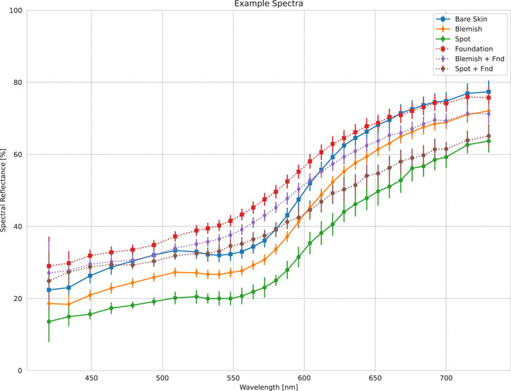
Figure 1. An selection of measured spectra from the data example presented in Figure 3. “Bare Skin” is the average spectrum from an area of clear skin on the model’s left cheek. “Spot” and “Blemish” are the average spectra from the dark spot and melasma on the model’s right cheek. “Foundation” is the “Bare Skin” area after application of makeup foundation
The data which we will use in this study comes from the HSI validation test carried out in March 2019. At that time, we conducted a study consisting of 3 foundation formulas applied to a group of 9 models as an end-to-end test of the HSI system. As products, we selected 3 makeup foundation products each with a different level of coverage as evaluated by expert sensory evaluation, and for the models we selected 9 models with a higher density of spots from our regular panel of models. We did not attempt to select the models based on skin tone.
For each product, we captured a hyperspectral image of each model before

Table 1. Test protocol used in the HSI validation study.
The HSI validation dataset contains a large amount of data in which we applied makeup foundation products with known coverage levels, and so it provides the perfect stage on which to develop new methods for the analysis of makeup coverage. As discussed in the introduction, we propose a new method for evaluating makeup foundation coverage based on the analysis of the distribution of spectral differences within the face before and after the product application. We show real examples of the spectra of various skin features before and after application of a makeup foundation in Figure 1. When we speak of the difference between the spectra of such features, the first parameter which we can look to is the spectral angle,
where
In this respect
Aside from classification, another way in which to use the spectral angle is to analyze the appearance of spots and the homogeneity of the skin over a given area by looking at the distribution of spectral angles within the region. This is not dissimilar from the idea behind using the volume of the
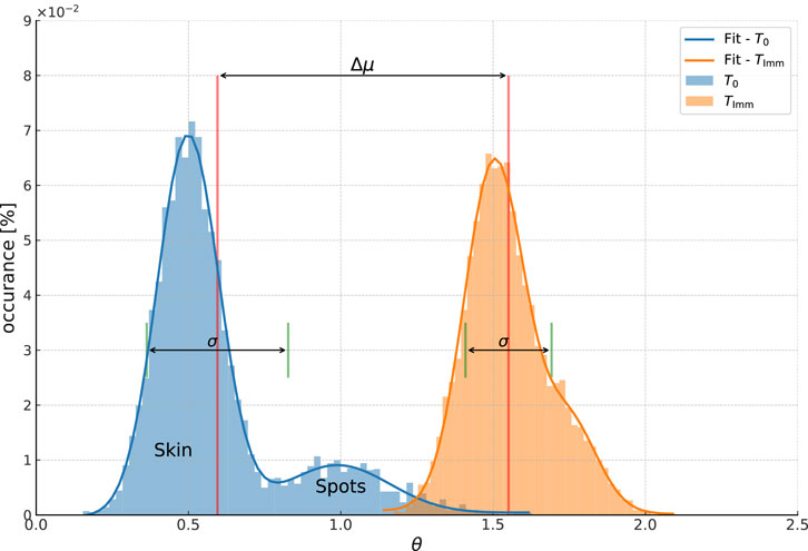
Figure 2. Conceptual example of the spectral angle distribution in a ROI. The blue peak is the distribution of spectral angles
First, there will be a peak near zero containing all the pixels which have a spectrum near the average bare skin, labeled “Skin” in the figure. The peak will not be at zero, because the dot product between two spectra in Equation 1 must be positive valued, meaning that only pixels with a spectrum which is exactly the average will give a spectral angle of zero. The greater the typical difference between each spectrum and the average bare skin spectrum, the higher will be the mean value. At the same time, the wider the range of spectra in the ROI, the greater the width of the distribution. The peak position and the peak width therefore tell us about the homogeneity of the skin in the ROI.
At the same time, the areas which have distinctly different spectra from the average will give a larger spectral angle, creating one or more peaks to the right of the skin peak. We have labeled this peak as spots as it corresponds to the features such as pigmented spots, moles, etc. In principle, there will be one peak for each type of feature in the ROI, but in practice the ability to separate them will depend on their distance from one another and on the width of the feature spectral distribution, that is the variation of spectra within each feature. Importantly, the separation of the skin and spots peaks gives us information about the degree of contrast between the spots and the base skin.
Now let us consider what happens when we apply a makeup foundation. First, the foundation changes the apparent color of the bare skin. At the same time, the hope is that the spots become less visible, that is to say closer in spectrum (color) to the skin. If we again take the spectral angle between each spectra in the ROI and this average spectrum, we will get a distribution of angles like that shown by the orange-yellow curve in Figure 2. As the base skin color changed, this registers as an increase in
In addition, as the spots are now closer to the base skin color, the spots peak begins to merge with the skin peak. If we consider the limit of a perfect spot hiding product, there would be only one peak after product application, as the spots would be indistinguishable from the skin. The most powerful way to analyze this effect is to characterize the entire spectral angle distribution. Doing that, we can estimate parameters such as the area of spots before and after product application, the contrast between the spots and the base skin, the relative change in color of the spots and the skin, etc.
At the same time, this distribution is only for one, arbitrarily selected, region. Looking at a different region will give us a different distribution, say, for example, if the there are more spots in one area than in another. The degree of difference in the spectral angle distribution from one region to the next tells us about the evenness of the skin at the scale of the region size. So, in order to truly characterize the product effect we should in principle also study how the distribution changes over the face. We will come back to this topic later in our discussion.
For a first, simple, evaluation of makeup foundation coverage, on the other hand, we can attempt to use the width of the spectral angle histogram in one ROI. Functionally, we will focus on the number of different spectra over a large ROI and ignore the spatial evenness of the color. The standard deviation of the spectral angle histogram would be the natural choice to do this, but we would then not benefit from the additional knowledge of the shift in the mean of the distribution.
To make use of that information, we can use a different reference spectra to ask a slightly different question. We previously compared the spectra in the ROI at
We therefore have two measurements using two different reference spectra:
In the next sections, we will apply this approach to the analysis of actual data from the HSI validation study. Doing so, we will see that the change in the spectral angle distribution caused by a makeup foundation looks like the theoretical example we considered so far and that we can indeed see a clear difference between the effect of different products.
So far we have discussed a theoretical model for coverage analysis based on the distribution of
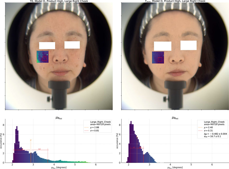
Figure 3. On the left, we show the
We show these spectral angle results overlaid on a reconstructed color image (under CIE D65 illumination (ISO/CIE, 1999)) at the top of the figure. In the overlay, more blue values indicate lower spectral angles, while more yellow values indicate higher spectral angles, i.e., regions which are more different from the reference spectrum. At the bottom of the figure, we show a histogram of the spectral angles in the ROI with the same color map applied. Before application of any product, at
Now, we do the same analysis after application of the High coverage product using the average spectrum at
The natural question which follows is whether we can differentiate the products using this approach, and to answer this question we show the same analysis for the Low and Medium coverage products in Figure 4. At first glance, the product effect on the
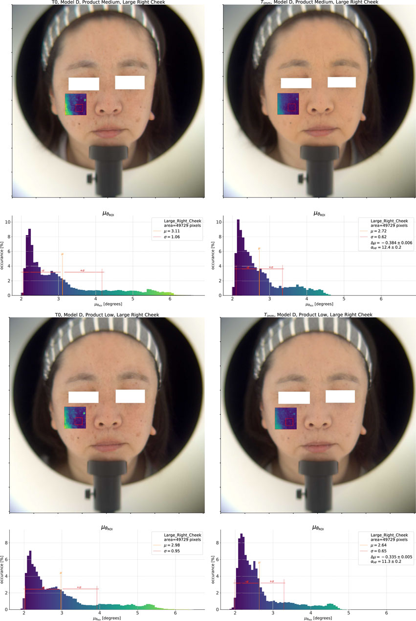
Figure 4. Top pane: Spectral homogeneity effect for the Medium coverage product. Bottom pane: Low coverage product.
Aside from the color homogeneity, we can also look at the color change. In Figure 5, we show a similar analysis of the spectral angle within a given ROI as in the last section. The key difference here is that instead of taking the average spectrum from the “Right Cheek” ROI at each time point as the reference spectrum, we instead use the average spectrum at
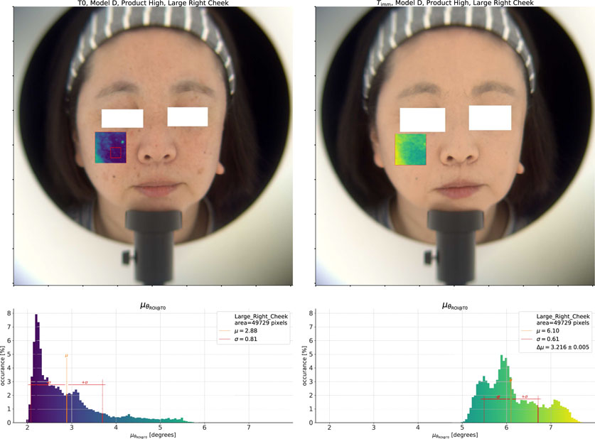
Figure 5. Analysis of the spectral change effect for the High coverage product. On the left, we show the
At the same time, we can also see that the difference in spectral angle between the base skin and the spots has reduced, as evidenced by the decrease in
As before, it is important to compare the effect of different products to sharpen our understanding. We show the same color shift analysis for the Medium and Low coverage products in Figure 6. Focusing on the Medium result, we can immediately see that the total color change effect is lower than that of the High coverage product (

Figure 6. Top pane: Analysis of the spectral change effect for the Medium coverage product. Bottom pane: Low coverage product.
Our goal is to apply this methodology to a large dataset. Ideally, we would conduct a full analysis of the spectral angle distribution for each study sample, but doing so requires us to develop methods for automating the analysis (including the non-trivial handling of edge cases) and agglomerating results over samples. As a short term approach, we propose the creation of simple parameters which we extract from each spectral angle distribution in order to compare one product to another.
In this context, we propose a Homogeneity Factor defined using the spectral angle distributions at
where
We would like to note that, even if the improvement of the homogeneity of the skin over the face due to a product is the main driver of what is typically called coverage, it is certainly not the sole factor influencing this attribute. For one, we expect not only the homogeneity of the color, by which we mean the number of different colors present in the region, to play a leading role, but also the color evenness, or the change of color from area to area, to impact the perception of coverage. Since attributes like homogeneity and evenness are objective measurements, while coverage is a loaded term with significant differences in user preference and perception between groups, it is also therefore best to avoid giving the latter label to an instrumental measurement. We have therefore chosen to call
As a measure of the overall change in spectra within the region after product application, we will likewise define a Spectral Shift Factor, which for now we will simply define as the difference in mean spectral angle referenced to the average spectrum at
Our expectation is that this parameter will follow closely the
In the original validation study analysis, we ranked the products according to the values of
For each model, we define a “Large Right Cheek” ROI of 35 by 35 mm as our working ROI, and a 12 by 12 mm “Right Cheek” ROI as the source of the reference spectrum to compute
After defining the ROI, we calculate the spectral angle for each pixel in the working ROI for each time point. The spectral angle with reference to the average spectrum in the “Right Cheek” at that time point gives us
We show box plots of the
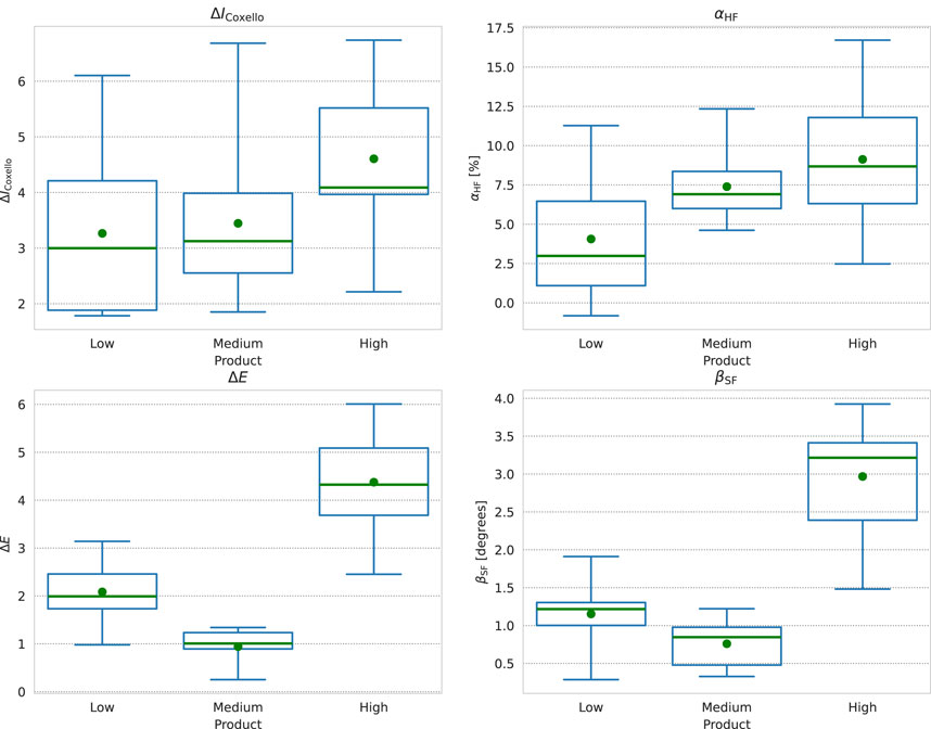
Figure 7. Box plots of (from top-left, clockwise)
As we expect, the overall trend in the two parameters is the same. The width of the distribution of
The
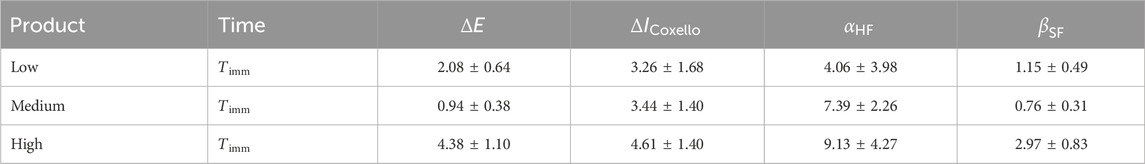
Table 2. Summary of results for the Large-Right-Cheek ROI after product application. We report each value as the mean
The
Next, we evaluated the statistical significance of the difference in measured values between products using the Python Statsmodel (Seabold and Perktold, 2010) library implementation of the Analysis of Variance (ANOVA) algorithm (Fisher, 1921) to determine if we can reject the null hypothesis (that no difference exists), followed by pairwise Multiple Comparison of Means (Tukey HSD) (Tukey, 1949) to group the products into statistically distinct subsets (if warranted). Here we used a test significance of 0.05 for both the ANOVA and the Tukey HSD tests. We give the result of this statistical analysis in Table 3. We find three distinct and consistent statistical groups for
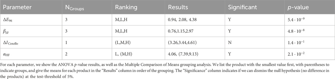
Table 3. Statistical analysis of products grouped by
For
The grouping results depend on the order in which we construct the samples, however, indicating that the model-to-model variability in the homogeneity effect is important. This raises the question of whether the variability between models is a inherent feature of attempting to correlate coverage with spectral homogeneity, or if there are some confounding effects for which we are not accounting. We will discuss this point further in the next section.
We find that, when averaged over all models, the sensory coverage evaluation correlates well with the change in spectral homogeneity after application, parameterized by
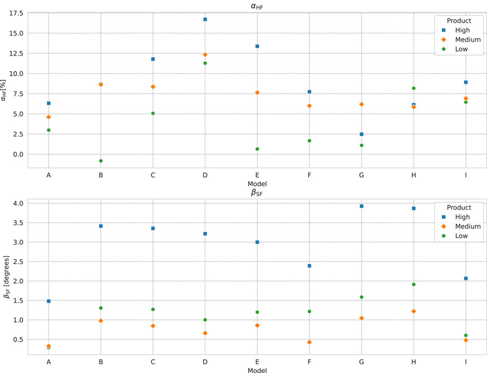
Figure 8. Plot
If it seems difficult to envision that the addition of a color-correcting film on top of the skin can decrease the homogeneity, it is important to keep in mind that the homogeneity we are talking about is the number of spectra in the region and their degree of difference. This determines, but is distinct from, the number of colors in the area and the
To further understand the
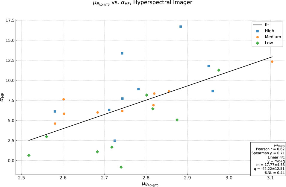
Figure 9. Plot of correlation between
The fact that the ordering (ranking) of the products by
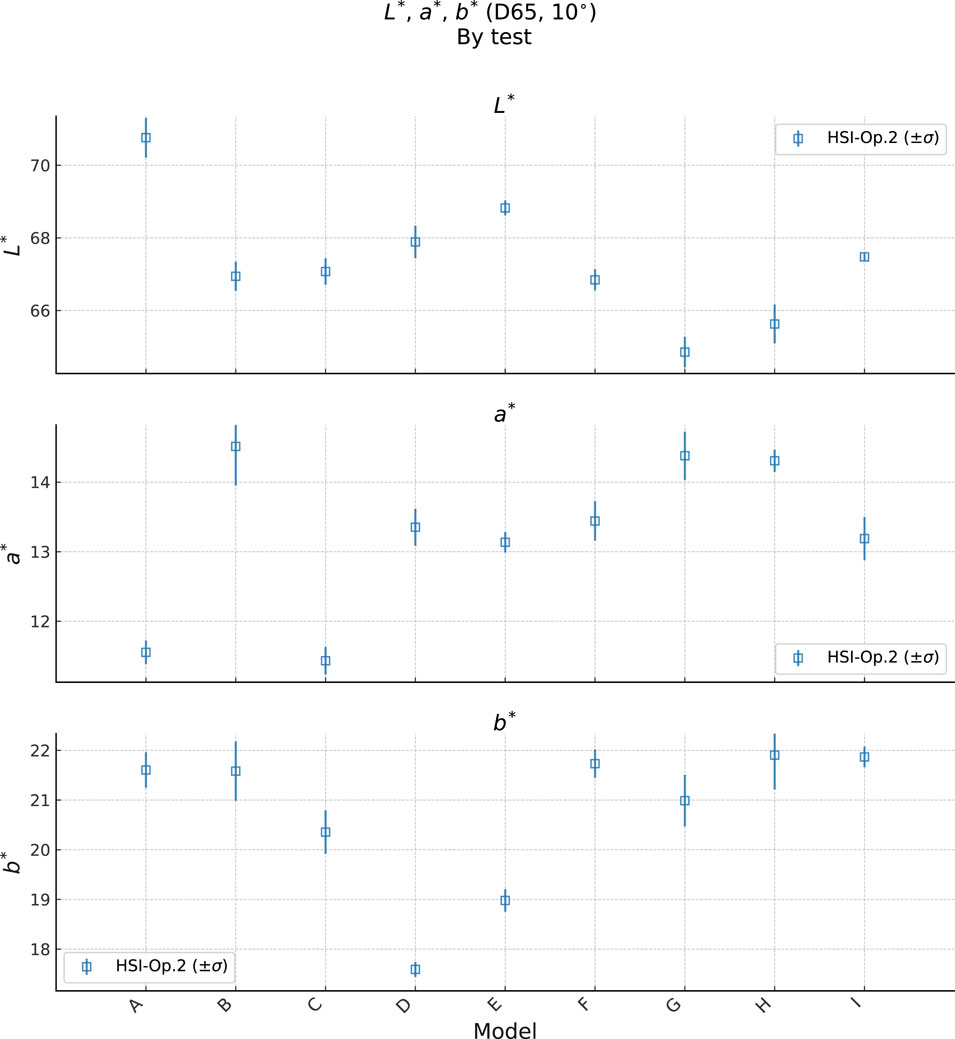
Figure 10. Plot of bare skin
It is important to keep in mind here that the
Looking at the spectral shift,
Considering that, it is interesting to look at the relationship between
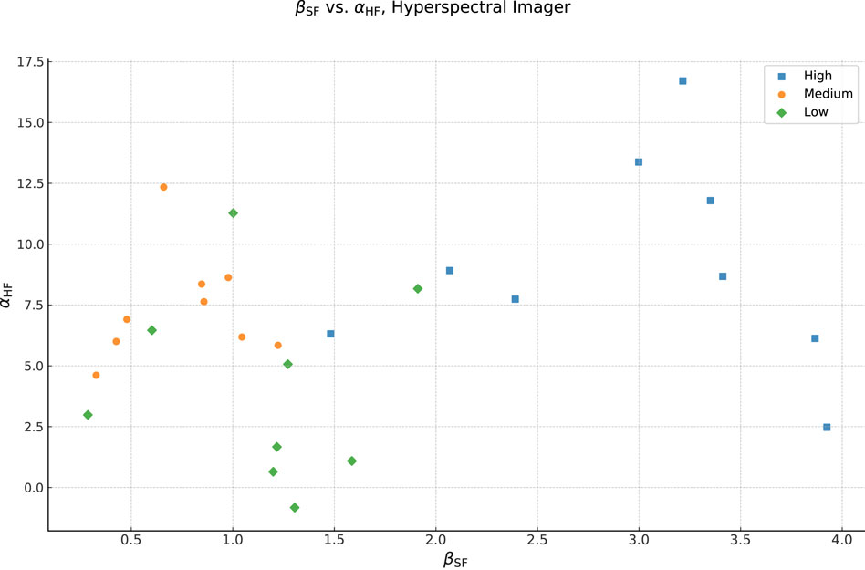
Figure 11. Correlation of the
As we discussed so far, these results are when applied to the average bare-skin
As a concrete example, the current study design applied 3 products to 9 models of various skin tones, giving 9 samples per product with minimal control over shade matching effect. A possible future test design could instead apply 3 products to 3 models of the same skin tone over 3 shade groups to give 9 samples per product, grouped by shade. We could then construct a relative ranking between products and map them for a constant panel of models. As the magnitude of the homogeneity change varies from model to model, however, it is difficult to conclude an absolute coverage value for a product independent of its application to at a specific model (just as an object under a specific light determines color, a product on a given skin determines absolute coverage).
This leads us back to a previous point, that the magnitude of the homogeneity effect depends on where we look, that is the ROI which we use for the measurement. Consider simply that the result from an ROI which includes a strongly pigmented spot and another nearby ROI which does not include the spot will be different. Concretely, if we re-do our analysis over the validation dataset using the smaller “Right Cheek” region as our working ROI, we find that the magnitudes of the
In order to answer the question of which ROI is the correct one in which to evaluate the coverage, we should in principle repeat our analysis for every possible ROI and compare the result from each, that is to say that we should effectively look everywhere on the face and at all scales. Practically, we can do this by drawing a large enough number of ROI of random size at random positions throughout the working region (such as the full cheek). The different sizes of these ROI allows us to check the dependence of the homogeneity change on the size scale, while the randomized location accounts for the variability of features, such as spots, within the face. The variance of results (whether homogeneity, color, etc.) across ROI at a selected size scale tells us about the texture or evenness of the skin at that scale. For example, if we have a model with dense freckles, the variance of color for ROI of the same size as the freckles will be much higher than at a larger size ROI where we would be taking the average over a number of freckles and areas of skin.
As a final note, in this study, we explored only a univariate analysis approach. Given the relationship between the initial skin color and homogeneity and the homogeneity and color effect of the products, this data will benefit from an approach using multivariate analysis. In addition, while for this first attempt we used the mean value of the spectral angle to construct a simple homogeneity parameter, we expect analysis of the complete distribution of spectral angles within each ROI to provide greater discrimination and explanatory power. For this reason, we are currently working on combining analysis of the spectral angle histograms and additional statistics calculated from them with a multi-ROI analysis of the type discussed above.
In this study we have started unravelling the complex topic of makeup coverage. In the fullest sense, coverage is a perceived attribute, but from a purely optical perspective, we expect that the perception of coverage for makeup products comes from the color change caused by the product, the change in color homogeneity and evenness over the face after application, and the ability of the product to hide spots and other blemishes. As the previous instrumental measurements do not consistently correlate with coverage in a way which allows us to compare one product to another, we have begun exploring the new parameters and analysis methods made available by hyperspectral imaging.
As a starting point, we defined a homogeneity factor
To test these new parameters and the overall analysis method, we applied them to an existing dataset, containing data for three makeup foundation products of different coverage levels (based on sensory evaluation) applied to nine models. We found that
This variability in product effect manifests as both a change in the magnitude of effect from model to model with the relative ranking between the products preserved, and as a change in the ranking between products for some models. In the latter, we see hints that this is the influence of the relative color different between the model’s skin tone and the product shade. As a next step in understanding this, we propose to assign each model a skin tone classification according to their average skin color, and look at the homogeneity effect vs. skin tone vs. product shade. If we indeed see a relationship between the model’s skin-tone and the homogeneity effect then this has clear implications for the design of future tests.
Likewise, the change in effect magnitude between models relates to the simple fact that the degree of homogeneity change which can occur depends on the starting inhomogeneity, which also implies that the measured effect depends on the selected ROI. This goes back to the general issue we face of the systematic uncertainty in evaluation results due to ROI selection. In addition, our homogeneity parameter is a function of the number of different spectra (colors) in the region and does not take into account the spatial distribution of the color. Intuitively, the evenness or texture is likely an important part of the perceived coverage effect, and we should therefore include it in our evaluation of makeup coverage. We can tackle both of these points by employing an analysis over the space of all possible ROI at varying size scales, combined with analysis of the full distribution of spectral angles within each ROI.
We also foresee the extension of this coverage analysis to include the lasting of the coverage over time. From preliminary data over multiple time points, we know that we can see the change of the homogeneity and color shift effects over time. There are some issues regarding the design of a such a study which we must address, such as how to accelerate the makeup wear in a way which does not bias the results, but from an analysis perspective, the main work which remains it is to improve our basic analysis of coverage in the directions which we have outlined here.
The raw data supporting the conclusions of this article will be made available by the authors, without undue reservation.
The studies involving humans were approved by L’Oreal Research and Innovation. The studies were conducted in accordance with the local legislation and institutional requirements. The participants provided their written informed consent to participate in this study. Written informed consent was obtained from the individual(s) for the publication of any potentially identifiable images or data included in this article.
CB: Conceptualization, Data curation, Formal Analysis, Methodology, Software, Validation, Visualization, Writing–original draft, Writing–review and editing. KU: Data curation, Resources, Writing–original draft, Writing–review and editing. AN: Conceptualization, Funding acquisition, Project administration, Writing–original draft, Writing–review and editing. MC: Formal Analysis, Methodology, Writing–original draft, Writing–review and editing.
The author(s) declare that financial support was received for the research, authorship, and/or publication of this article. This work was funded by L’Oreal Research and Innovation.
The authors would like to thank Emilie Yokoyama for useful discussions on study conceptualization and assistance in proofreading this manuscript, Mie Yoshida for help in data collection, and Damien Velleman for department-level assistance regarding resource procurement and administration.
Authors CB, KU, and AN were employed by the company L'Oréal Research & Innovation.
The remaining author declares that the research was conducted in the absence of any commercial or financial relationships that could be construed as a potential conflict of interest.
All claims expressed in this article are solely those of the authors and do not necessarily represent those of their affiliated organizations, or those of the publisher, the editors and the reviewers. Any product that may be evaluated in this article, or claim that may be made by its manufacturer, is not guaranteed or endorsed by the publisher.
The Supplementary Material for this article can be found online at: https://www.frontiersin.org/articles/10.3389/fchem.2024.1400796/full#supplementary-material
Batres, C., Porcheron, A., Latreille, J., Roche, M., Morizot, F., and Russell, R. (2019). Cosmetics increase skin evenness: evidence from perceptual and physical measures. Skin Res. Technol. 25, 672–676. doi:10.1111/srt.12700
Blaksley, C., Casolino, M., and Cambié, G. (2021). Design and performance of a hyperspectral camera for full-face in vivo imaging. Rev. Sci. Instrum. 92, 055108. doi:10.1063/5.0047300
Blaksley, C., Udodaira, K., Cambié, G., Yoshida, M., Nicolas, A., Velleman, D., et al. (2022). Repeatability and reproducibility of a hyperspectral imaging system for in vivo color evaluation. Skin. Res. Technol. 28, 544–555. doi:10.1111/srt.13160
De Rigal, J., Abella, M.-L., Giron, F., Caisey, L., and Lefebvre, M. A. (2007). Development and validation of a new skin color Chart®. Skin Res. Technol. 13, 101–109. doi:10.1111/j.1600-0846.2007.00223.x
De Rigal, J., Des Mazis, I., Diridollou, S., Querleux, B., Yang, G., Leroy, F., et al. (2010). The effect of age on skin color and color heterogeneity in four ethnic groups. Skin Res. Technol. 16, 168–178. doi:10.1111/j.1600-0846.2009.00416.x
Fisher, R. A. (1921). On the “probable error” of a coefficient of correlation deduced from a small sample. Metron 1, 3–32.
Flament, F., Gautier, B., Benize, A.-M., Charbonneau, A., and Cassier, M. (2017). Seasonally-induced alterations of some facial signs in caucasian women and their changes induced by a daily application of a photo-protective product. Int. J. Cosmet. Sci. 39, 664–675. doi:10.1111/ics.12427
Haralick, R. M., Shanmugam, K., and Dinstein, I. (1973). Textural features for image classification. IEEE Trans. Syst. Man, Cybern. SMC-3, 610–621. doi:10.1109/TSMC.1973.4309314
Huixia, Q., Xiaohui, L., Chengda, Y., Yanlu, Z., Senee, J., Laurent, A., et al. (2012). Instrumental and clinical studies of the facial skin tone and pigmentation of Shanghaiese women. changes induced by age and a cosmetic whitening product. Int. J. Cosmet. Sci. 34, 49–54. doi:10.1111/j.1468-2494.2011.00680.x
ISO/CIE (1999). CIE standard illuminants for colorimetry. Standard: International Commission on Illumination.
ISO/CIE (2019). Colorimetry — Part 1: CIE standard colorimetric observers. Standard: International Commission on Illumination.
King, D. E. (2009). Dlib-ml: a machine learning toolkit. J. Mach. Learn. Res. 10, 1755–1758. doi:10.5555/1577069.1755843
Kruse, F. A., Boardman, J. W., and Huntington, J. F. (2003). Comparison of airborne hyperspectral data and eo-1 hyperion for mineral mapping. IEEE Trans. Geoscience Remote Sens. 41, 1388–1400. doi:10.1109/tgrs.2003.812908
Nishidate, I., Aizu, Y., and Mishina, H. (2004). Estimation of melanin and hemoglobin in skin tissue using multiple regression analysis aided by Monte Carlo simulation. J. Biomed. Opt. 9, 700–710. doi:10.1117/1.1756918
Python (2020). Python software foundation. Available at: https://www.python.org/(Accessed June, 2020).
QT (2020). The Qt company. Available at: https://www.qt.io/(Accessed June, 2020).
Seabold, S., and Perktold, J. (2010). “statsmodels: econometric and statistical modeling with python,” in 9th Python in Science Conference, Austin, Texas, June 28 - July 3, 2010, 92–96. doi:10.25080/majora-92bf1922-011
Speranskaya, N. (1959). Determination of spectrum color co-ordinates for twenty seven normal observers. Opt. Spectrosc. 7, 424–428.
Stiles, W., and Burch, J. (1959). N.p.l. colour-matching investigation: final report (1958). Opt. Acta Int. J. Opt. 6, 1–26. doi:10.1080/713826267
Tukey, J. W. (1949). Comparing individual means in the analysis of variance. Biometrics 5, 99–114. doi:10.2307/3001913
Vane, G., and Goetz, A. F. (1988). Terrestrial imaging spectroscopy. Remote Sens. Environ. 24, 1–29. Imaging Spectrometry. doi:10.1016/0034-4257(88)90003-X
Keywords: hyperspectral imaging, spectral imaging, spectral analysis, color evaluation, product evaluation
Citation: Blaksley C, Udodaira K, Nicolas A and Casolino M (2024) A new method for the evaluation of makeup coverage using hyperspectral imaging. Front. Chem. 12:1400796. doi: 10.3389/fchem.2024.1400796
Received: 14 March 2024; Accepted: 26 August 2024;
Published: 10 September 2024.
Edited by:
Jeroen Jansen, Radboud University, NetherlandsReviewed by:
Rosalba Calvini, University of Modena and Reggio Emilia, ItalyCopyright © 2024 Blaksley, Udodaira, Nicolas and Casolino. This is an open-access article distributed under the terms of the Creative Commons Attribution License (CC BY). The use, distribution or reproduction in other forums is permitted, provided the original author(s) and the copyright owner(s) are credited and that the original publication in this journal is cited, in accordance with accepted academic practice. No use, distribution or reproduction is permitted which does not comply with these terms.
*Correspondence: Carl Blaksley, Y2FybC5ibGFrc2xleUBsb3JlYWwuY29t
Disclaimer: All claims expressed in this article are solely those of the authors and do not necessarily represent those of their affiliated organizations, or those of the publisher, the editors and the reviewers. Any product that may be evaluated in this article or claim that may be made by its manufacturer is not guaranteed or endorsed by the publisher.
Research integrity at Frontiers
Learn more about the work of our research integrity team to safeguard the quality of each article we publish.