Deep neural network for prediction and control of permeability decline in single pass tangential flow ultrafiltration in continuous processing of monoclonal antibodies

Single-pass tangential flow filtration (SPTFF) is a crucial technology enabling the continuous manufacturing of monoclonal antibodies (mAbs). By significantly increasing the membrane area utilized in the process, SPTFF allows the mAb process stream to be concentrated up to the desired final target in a single pass across the membrane surface without the need for recirculation. However, a key challenge in SPTFF is compensating for flux decline across the membrane due to concentration polarization and surface fouling phenomena. In continuous downstream processing, flux decline immediately impacts the continuous process flowrates. It reduces the concentration factor achievable in a single pass, thereby reducing the final concentration attained at the outlet of the SPTFF module. In this work, we develop a deep neural network model to predict the NWP in real-time without the need to conduct actual NWP measurements. The developed model incorporates process parameters such as pressure and feed concentrations through inline sensors and a spectroscopy-coupled data model (NIR-PLS model). The model determines the optimal timing for membrane cleaning steps when the normalized water permeability (NWP) falls below 60%. Using SCADA and PLC, a distributed control system was developed to integrate the monitoring sensors and control elements, such as the NIRS sensor for concentration monitoring, the DNN model for NWP prediction, weighing balances, pressure sensors, pumps, and valves. The model was tested in real-time, and the NWP was predicted within <5% error in three independent test cases, successfully enabling control of the SPTFF step in line with the Quality by Design paradigm.

1 Introduction

The continuous processing of monoclonal antibodies (mAbs) is an area of rapidly growing interest in the biopharmaceutical industry. Currently, more than one hundred mAbs have been approved by the US FDA, and the annual worldwide market for mAbs is projected to rise to over $180 billion by 2025 (Jabra, Lipinski, and Zydney, 2021). Continuous processing has been shown to offer many advantages over traditional batch-mode manufacturing, including many-fold lower capital costs, higher throughput, and efficient utilization of consumables, water and energy. In order to switch from batch to continuous processing, each of the multiple unit operations involved in the manufacturing process, including cell culture, dead-end filtration, chromatography, viral inactivation, and ultrafiltration, need to be adapted and modified for continuous operation (Krippl et al., 2021). Continuous operation can be achieved in cell culture by using perfusion systems that allow continuous outflow of mAb-containing supernatant from the cell culture bioreactor over weeks of operation. For chromatography, continuity is achieved by increasing the number of columns to two or more operating in parallel. One column is always “loading” while the other cycles through “non-loading” steps. In the case of viral inactivation, continuity can be achieved by having two parallel viral inactivation tanks or switching to continuously flowing reactors for viral inactivation (Kateja et al., 2016). Finally, in the case of ultrafiltration, single-pass tangential flow filtration (SPTFF) has emerged as a critical technology which essentially uses a very long membrane to achieve high concentration factors in a single pass without the need for recirculation of the retentate back into the feed vessel, thus enabling continuous inline concentration.

Ultrafiltration is an essential and core unit operation as it directly influences the quality of the final product. While most ultrafiltration is done in batches, multiple studies have shown that continuous ultrafiltration (inline or single pass) may be successfully integrated into the continuous processing train. These single-pass tangential flow filtration (SPTFF) devices help save space and boost the efficiency of succeeding operations by eliminating the need for several pump runs, which may lead to protein aggregation in batch systems. Several SPTFF modules, created in response to market demand over the previous several years, are now commercially available. Single-use systems like Pall’s Allegro^TM and Millipore Sigma’s Mobius^® FlexReady Solution for tangential flow filtration (TFF), as well as Repligen’s TangenXTM SIUSTM and others, are just a few examples (Thakur et al., 2022). Creating and testing a cleaning and sanitization cycle is unnecessary since these single-use systems are already sterile before usage. However, these disposable systems are primarily intended for batch operations in which the feed solution is cycled through the module several (repeated) times to obtain the desired concentration. Several experimental investigations have been published that demonstrate the efficacy of SPTFF in producing mAbs (Kaiser et al., 2022).

However, several process control and integration issues must be addressed before SPTFF technology can be incorporated into continuous manufacturing units. The SPTFF membrane mass transfer can be affected by concentration polarization and the formation of the gel layer on the membrane surface. This leads to membrane fouling (Figure 1). Membrane fouling seems to be the most significant disadvantage of membranes, which must be prevented or reduced (Jerez et al., 2008). Once it begins to develop, this phenomenon severely compromises the long-term functionality of membranes (Stoller and Serrão Mendes, 2017). The effect is evident concerning the change in normalized water permeability. When the normalized permeability of the membrane drops below 60%, it can only be recovered by cleaning, which directly impacts the integration of SPTFF into the continuous platform.

FIGURE 1

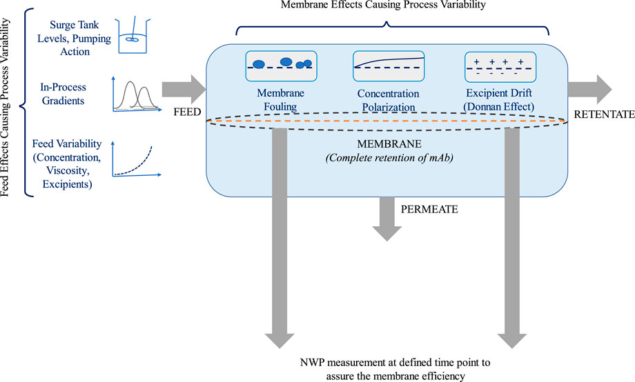
FIGURE 1. Illustration showing the various causes of membrane fouling.

Few mechanistic methods have been published in the papers to anticipate concentration polarization, gel layer formation and fouling parameters (Chew, Aroua, and Hussain, 2017), which can be altered and implemented in the continuous processing train with SPTFF control. More specifically, the reports have also shown the utilization of the theory of boundary flux to control the fouling (Stoller and Serrão Mendes, 2017). However, it takes considerable time and effort to include mechanistic models in the process stream when they are implemented in real-time.

Artificial intelligence (AI) and deep learning (DL) have had a significant impact on a variety of fields over the past several decades, beginning with web search engine optimization, self-driving systems, computer visions, and optical character recognition (Srinidhi, Ciga, and Martel, 2021). Recent years have seen the introduction of deep learning approaches into manufacturing, empowering them with enhanced control architecture and prediction-based process optimization solely based on historians. However, the biopharma industry has yet to completely embrace deep learning-based strategies to migrate to Industry 4.0. Notably, the use of regression models is not new to the ultrafiltration procedure, and multiple publications have shown the use of a multilayer neural network model for predicting flux/total resistance and rejection during ultrafiltration (Razavi, Mortazavi, and Mousavi, 2003). In the last 2 decades, AI has been demonstrated to offer an alternate approach for accurately simulating these membrane processes. The commonly used AI-ML techniques include artificial neural network (ANN), fuzzy logic, adaptive neuro-fuzzy inference system (ANFIS), genetic programming, and support vector machine (Dornier et al., 1995; Kim et al., 2009; Cho et al., 2010; Madaeni and Kurdian, 2011; Rahmanian et al., 2011; Rahmanian et al., 2012; Salehi and Razavi, 2012; Shokrkar et al., 2012; Shokrkar et al., 2012; Fazeli et al., 2013; Khayet and Cojocaru, 2013; Barello et al., 2014; Rahimzadeh, Ashtiani, and Okhovat, 2016; Salehi and Razavi, 2016; Adib, Raisi, and Salari, 2019; Nejad et al., 2019). ANN is the most often utilized for modelling membrane separation (Jawad, Hawari, and Javaid Zaidi, 2021). To improve prediction accuracy and reduce prediction time, however, an enhanced variant of ANN, known as a deep neural network, was constructed, and this has been used in this study.

In this paper, a deep-learning regression model is developed and used to predict the membrane’s NWP at various time points and process designs. The model was anchored using an inline NIR probe, DCS, and control software written in Python. The DCS regulates the pump and plans a cleaning cycle based on the NWP forecast without disrupting the process stream. This work leverages process analytical technology (PAT) and ML to enable automated, integrated, and well-controlled STPFF operation. In line with the US FDA’s PAT and Quality by Design (QbD) paradigms, the proposed approach utilizes product and process understanding to adjust process parameters to consistently meet CQA targets, incorporating flexibility and robustness without frequent human intervention.

2 Materials and methods

2.1 Materials

The monoclonal antibody (mAb) employed in the research is an immunoglobulin G1 (IgG1) antibody with a molecular weight of roughly 150 kDa and a pI of 8.5. The 0.6 g/L mAb concentration in the shake flasks yielded 3 L of cell culture harvest. Glycine, Tris, sodium chloride (NaCl), sodium dihydrogen phosphate (NaH₂PO₄), disodium hydrogen phosphate (Na₂HPO₄), and sodium hydroxide (NaOH) were procured from Merck, India. All materials were of analytical quality. Deionized water was used to make buffer solutions.

2.1.1 SPTFF materials

The following steps were taken to obtain the ultrafiltration experiment material from the harvest cell culture fluid. The harvest was taken from −20°C thawed at 4°C below freezing, raised to room temperature, and then filtered at 0.2 μm. Filtered harvest was placed into a column equilibrated with a 20 mM phosphate and 150 mM NaCl buffer at pH 7.4 and packed with MabSelectSure^TM resin (GE Healthcare, Sweden). The scattered components were washed in an equilibration buffer. The product was eluted in a glycine HCl buffer of 100 mM concentration at pH 3.5. After that, 50 mM NaOH and 1 M NaCl were used as cleaning buffer for flushing the column in situ. Subsequently, the pH was held at 3.5 for 1 h before being neutralized to pH 7 using 2 M Tris buffer, effectively killing any remaining viruses. The sample was further processed using anion exchange chromatography according to in-house protocols. For the ultrafiltration studies, a total volume of 2 L of the final drug material in a glycine Tris buffer of pH 7 with a total concentration of 8.5 g/L was obtained.

2.2 SPTFF experimental setups

SPTFF was accomplished with a Cadence Inline Concentrator (ILC) module (Pall Corporation, United States), while diafiltration was performed with a Cadence Inline Diafiltration (ILD) module (Pall Corporation, United States). Membranes of regenerated cellulose with a molecular weight cutoff of 30 kDa were used in their construction. The ILC module was comprised a total of seven 0.0093 m² membranes for a combined membrane area of 0.065 m². Three parallel membranes were connected in series to two parallel membranes connected in series to complete the internal staged flow channel. This 4-in-series design was chosen among the various Cadence ILC configuration possibilities available by Pall Corporation, including 7-, 8-, and 9-in series because it has the smallest total membrane area and is, therefore, best suited for low-volume applications (Thakur et al., 2022).

In the study, three distinct concentration-specific process modules were designed. In the first process design (Figure 2A), a single feed pump, a peristaltic pump, was used to pump feed material from the tank to the membrane. The retentate and permeate were then collected in separate containers. To prevent pressure building in the second design, the peristaltic feed pump was replaced with a quaternary pump (Figure 2B). Feed and permeate peristaltic pumps were employed in the final process design (Figure 2C) to carry feed samples with a high concentration. In each module, the feed pressure, permeate pressure, retentate pressure, flow rate, and concertation were recorded every 2 s at a constant interval. The concentration of the feed is measured using the NIR-based PAT instrument, which is briefly described in the following sections.

FIGURE 2

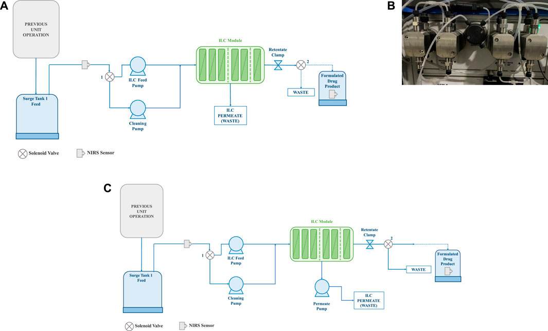
FIGURE 2. (A) Process design with single pump (only feed pump design); (B) Quaternary pump used in the second process design; (C) Process design with both feed pump and permeate pump (1- Solenoid valve 1 and 2—Solenoid valve 2).

2.3 NWP experiments

To obtain various outcomes that would be used in the model development for process monitoring and control, the normalized water permeability of the membrane was measured at varying times under different process circumstances. In addition, a large number of data points are required for a precise model to be developed. The NWP was measured at 20°C over the transmembrane pressure for a given membrane and can be expressed as follows:

$NWP=\frac{Permeateflux\left(LMH\right)}{TMP\times A}\times TCF$

$TMP=\frac{P_{feed}+P_{retentate}}{2-P_{permeate}}$

$TCF=\frac{{\mu }_{water@{20}^{0}C}}{{\mu }_{water@{25}^{0}C}}$

Where, $TMP$ is transmembrane pressure, $A$ is membrane area, $TCF$ is temperature correction factor at 20°C, $P_{feed}$ is feed pressure, $P_{retentate}$ is permeate pressure, $P_{permeate}$ is permeate pressure, ${\mu }_{water@{20}^{0}C}$ is viscosity of water at 20°C and ${\mu }_{water@{25}^{0}C}$ is viscosity of water at 25°C. Before the process began, the feed and filtrate flux of the pure water was measured prior to initiating the ultrafiltration (UF) process, and the resulting flux was adjusted to 100% NWP.

2.4 Near infrared spectroscopy (NIRS) based PAT

NIRS methods for quantifying analytes are developed by training a chemometric algorithm with a library of spectra containing known concentrations within the intended measurement range. A NIRS calibration library was built for the mAb in the current buffer of 20 mM phosphate and 100 mM NaCl at pH 7.4. The library was constructed using an Antaris^TM II FT-NIR Analyzer (Thermo Fisher Scientific, United States). The spectrum was recorded using a Series 750 Transmission Flow Cell (Thermo Fisher Scientific, United States). All spectrum measurements were taken between 4,000 and 1,000 cm⁻¹. The calibration spectra were acquired in triplicate with a resolution of 2 cm⁻¹ and a mean of 16 scans. In order to compensate for variations in mAb concentration between 0.5 and 60 g/L, a system of calibration standards was developed. Initially, 5 mL of mAb sample at 60 g/L was generated by concentrating the mAb material. After that, the solution was diluted serially with a buffer while calibrating spectra were taken at each stage. The dilution method was designed to achieve a final concentration of 0.5 g/L by diluting the solution by a factor of 1.0 at each stage. Additionally, a UV spectrophotometer and a microplate reader were used to confirm the concentrations of the calibration standards offline. Using a weight-based dilution method, samples were adjusted to achieve a UV absorbance value in the range of 0.5–1. The coefficient of extinction for mAb was 1.60.

TQ Analyst 9.5 (Thermo Fisher Scientific, United States) software was used to develop a partial least square (PLS) model to extract concentration data from NIRS spectra. Figure 3A depicts the outcomes of calibrating the calibration library and PLS model. A 33-point Savitsky-Golay smoothing filter was implemented after averaging duplicate spectra. As per the NIRS spectral area, a calibration model was developed between 4,000 and 11,000 cm⁻¹. The model was verified using 15 validation standards chosen randomly from the 90 standards in the library. When using this model, a correlation coefficient of 0.99 was found. Ten samples were generated for external validation, and the calibrated model reliably predicted the mAb concentration to be within 0.5 g/L. The calibrated model was generated as a method file and then put into a real-time spectral collecting and processing workflow developed with Thermo Fisher Scientific’s Result software (Figure 3B). The workflow began with the triggering of the collection of NIRS spectra from the two sensors at regular one-minute intervals, continued with the automatic transfer of the spectra to the calibration models, and concluded with the reporting of the numerical concentration measurement result in a time-stamped text file accessible via local area network (LAN) by the central control system.

FIGURE 3

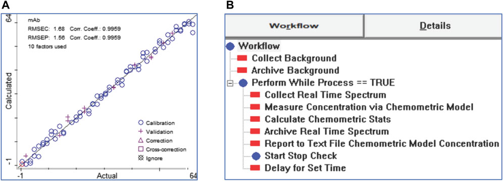
FIGURE 3. (A) Calibration of a chemometric model with NIRS spectra for the measurement of mAb concertation; (B) A workflow for the acquisition and analysis of spectra in real-time using the Result software.

2.5 Deep neural network (DNN)

The common belief is that simple models are better at achieving higher interpretability than complex models. This belief can be attributed to the widespread use of linear and basic decision tree models in various applications. However, recent advancements in the field have challenged this belief (Montavon et al., 2018), and precise interpretation techniques have enabled the understanding of complex machine learning models, including deep neural networks (DNNs). In this study, a deep neural network (DNN)-based enabler that could be incorporated into the forthcoming digitalized biopharma umbrella is developed. DNN is an artificial neural network (ANN) that includes multiple dense hidden layers between the input and output layers (Natarajan et al., 2021). Incorporating depth (increasing the number of dense layers) in a network architecture enables the modelling of complex non-linear relationships. The deep learning model can learn from process conditions by using multiple hidden layers, leading to the prediction of target values. The hidden layer consists of neurons (dense layer units) that execute mathematical operations on input data. The pivotal hyperparameters in DNNs include the learning rate, optimizer, activation function, epochs, and batch size.

Activation functions are crucial in neural networks as they introduce nonlinearity. The nonlinearity of neural networks enables the development of intricate representations and functions from inputs, which is unattainable with a basic linear regression model (Parhi and Nowak, 2020). Optimizers are algorithms that modify neural network attributes, including weights and learning rate, to minimize losses and enhance accuracy. The learning rate is a hyperparameter that regulates the magnitude of model adjustments in response to estimated errors during weight updates. In addition, the number of batch size, epochs, dropout layers and leaky layers enhance the model’s performance. The batch size is a hyperparameter specifying the number of samples used to update the internal model parameters. The hyperparameter “epochs” determine how many iterations the learning algorithm will perform on the training dataset. The leaky rectified linear unit (ReLU) is employed to enhance model stability by mitigating the issue of output values of 0 and the dying ReLU problem that may arise during neural network training. Several studies (Masum et al., 2021; Pirrung et al., 2017; Yegnanarayana, 2009; Zou et al., 2009) offer extensive information on hyperparameters and mathematical insights into DNN. The DNN model’s hyperparameters were optimized using the Bayesian optimization (BO) algorithm. The DNN architecture is depicted in Figure 4.

FIGURE 4

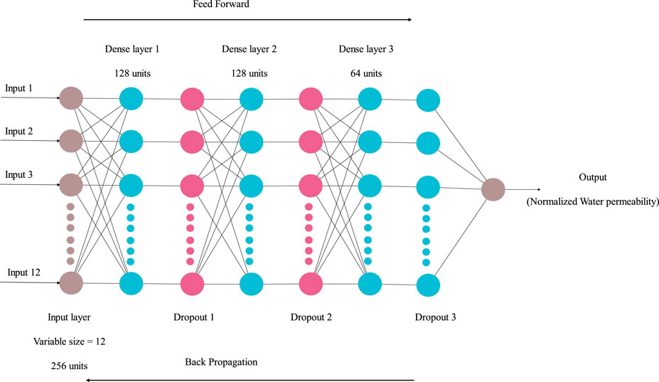
FIGURE 4. Deep Neural Network architecture.

2.6 Bayesian optimization

A collection of ideal hyperparameters permits performance enhancement and prevents performance concerns such as overfitting. As mentioned in the above section, the deep neural network model parameters were hypertuned using the go-to optimization algorithm, the Bayesian optimization algorithm. Probability is a fundamental concept heavily utilized by statistical and machine learning algorithms, among other methodologies. It could predict the outcomes of regression and classification problems. The utilization of conditional probability, Bayes’ theorem, and the Gaussian distribution enable the prediction of the likelihood of a specific class or value based on a given set of inputs. The duo can be utilized in a technique referred to as Bayesian optimization (BO) to optimize the hyperparameters of a machine learning model. Bayesian optimization is a stochastic optimization method that seeks to minimize an objective black box function on a global scale (Masum et al., 2021). The global depreciation only applies to certain constrained sets. The function of the black box is stated in the equation:

$f:\mathbb{X}\to R$

Where, $f$ is the function, $\mathbb{X}$ is the domain, and $R$ is the co-domain (range).

Researchers have elaborated on the mathematical aspects of Bayesian optimization (Frazier, 2018a; Frazier, 2018b). The BO framework comprises three essential elements: the surrogate model, the Bayesian updating process, and the acquisition function. After each new assessment of the objective function, the surrogate model is updated using the Bayesian updating process to ensure that it fits all points of the objective function. The acquisition function then evaluates the evaluation.

The BO framework comprises three essential components: the acquisition function, the Bayesian updating process, and the surrogate model. The Gaussian process is frequently employed as a surrogate model in Bayesian optimization. This allows it to specify a prior function that could be used to enhance future predictions of the goal function during a learning process. Acquisition functions, on the other hand, are responsible for predicting where within the search space to collect samples. The “exploration and exploitation” approach serves as the foundation for the acquisition function. With the help of this function, the optimizer can use the optimum zone until a better value is discovered. The goal is to maximize the acquisition function to identify the location of the following sample. The upper confidence bound and Thompson’s sampling are founded on the same conceptual framework. More mathematical insights on BO are given in published articles (Frazier, 2018a; Frazier, 2018b).

2.7 Model evaluation criteria

The model performance was evaluated using different statistical criteria, including coefficient of correlation, variants of coefficient of correlation, mean absolute error (MAE), mean squared error (MSE), root mean squared error (RMSE), normalized root mean squared error (NRMSE), Akaike information criterion (AIC) and Bayesian information criterion (BIC) (Nikita et al., 2022; Chhabra et al., 2023).

3 Results and discussion

3.1 Deep neural network model hypertuning

Hyperparameter tuning is a fundamental part of a deep learning project (Koehrsen, 2018). There are two types of hyperparameters: structural hyperparameters and optimizer hyperparameters. The structural hyperparameters in the DNN are the number of dense layers, layer units, activation function, leaky layers, and loss function. The optimizer hyperparameters are the type of optimizer, epochs, batch size and learning rate. Due to the high computational demands of deep learning models, conventional hyperparameter optimization methods such as grid search and random search are frequently inefficient and time-consuming. Furthermore, these techniques leverage the model’s prior knowledge gained from previous optimization iterations. Bayesian optimization employs previous optimizations to generate a hyperparameter list that is highly optimized and requires fewer samples to attain optimal performance. This study’s model was hypertuned using the Gaussian process (GP) as the surrogate model and expected improvement (EI) as the acquisition function. The BO algorithm was implemented in Python using the Spyder integrated development environment (IDE) for deep neural network (DNN) hyperparameter tuning. The algorithm was implemented with Python libraries such as Keras, Bayes-opt, NumPy, Sci-Kit learn, TensorFlow, Pandas, and SciPy. The initial stage of hypertuning involves developing a training pipeline for the deep neural network utilizing the dataset and adjustable hyperparameters. The subsequent stage consists in formulating an objective function that encapsulates the training and inference of the network, serving as the Blackbox, and transforming the inference into an evaluation metric that can be utilized in the optimization procedure. A reliable signal is necessary for the solver to assess sampled points. The function is used in a Bayesian optimization process at a global level. The Python environment utilizes the Bayes-opt package to process the aforementioned workflow. The model’s performance was evaluated using specific hyperparameters through a five-fold cross-validation technique with fifty iterations. The hyperparameters range and hypertuned hyperparameters are shown in Table 1.

TABLE 1

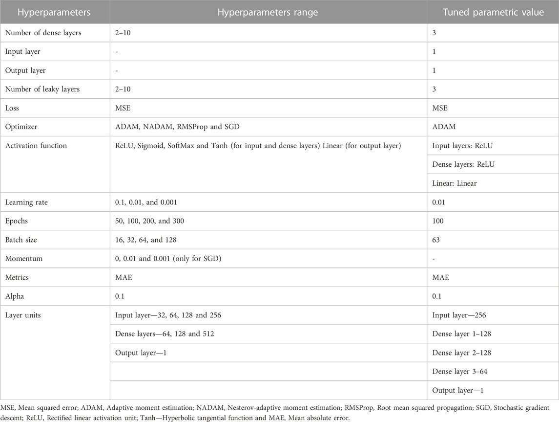
TABLE 1. DNN model hyperparameters range and hyperparameters used for model development.

3.2 Deep learning model development

The hypertuned neural network-based deep learning regression model was developed in Python using TensorFlow, Keras, NumPy, Pandas, and Sci-Kit learn packages. The study employed the Adam optimizer, a significant hyperparameter, in developing a deep learning-based neural network model. The Adam optimizer is a stochastic gradient descent algorithm that utilizes adaptive estimation of first- and second-order moments. It is designed to adapt the learning rate of each parameter by using the first and second moments, which are approximations of the gradient’s mean and variance, respectively. It is a widely utilized optimization algorithm in the field of deep learning due to its notable effectiveness and efficiency. The Adam optimizer has demonstrated superior convergence rates compared to alternative stochastic gradient descent techniques. The other hyperparameters used in the model development are given in Table 1. The developed model was trained using eighty percentage of the experimental data selected randomly, tested using the remaining data sets and cross-validated (repeated k-fold model cross-validation). During DNN model training, 20% of the training dataset was used for validation. The model was built with twelve input parameters that directly/indirectly influence NWP in some way. The model input parameter includes experimental module, feed concentration, feed pump flow rate, volumetric concentration flux (VCF), permeate pump, total module run time, initial feed pressure, initial retentate pressure, initial permeate pressure, steady-state feed pressure, steady-state retentate pressure and steady-state permeate pressure. The neural net learns from input parameters and predicts the NWP at a given condition. The model evaluation scores show that the developed model is precise and robust. The evaluation scores are given in Table 2.

TABLE 2

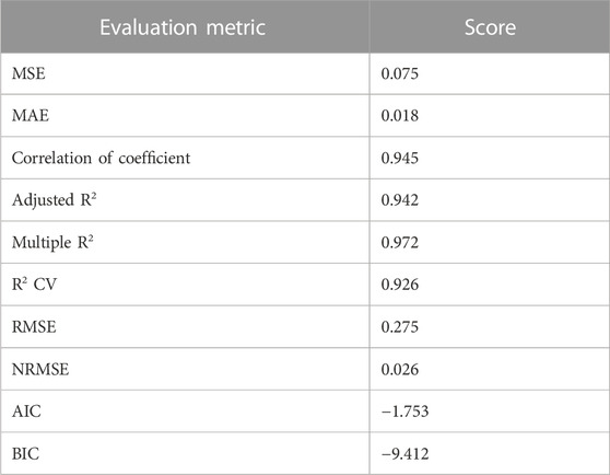
TABLE 2. Model evaluation metric scores.

The loss function is computed over all data items during each epoch to determine the quantitative loss at the given epoch. To get further understanding, validation loss is shown with training loss (Figure 5A). It is observed that the model’s performance in terms of the loss function and mean absolute error is comparable to training and validation datasets. The results support the resilience of the model.

FIGURE 5

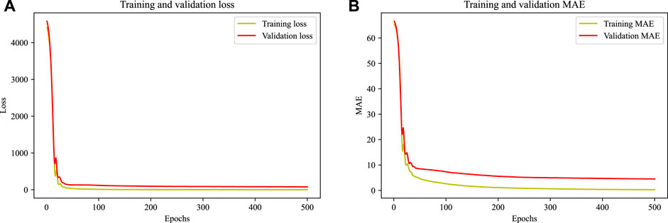
FIGURE 5. (A) Training and validation loss plots (B) Training and validation mean absolute error plots.

The DNN model was assessed using various statistical measures such as R², Adj. R², Multiple R², CV R², MAE, MSE, RMSE, NRMSE, AIC, and BIC. Statistical criteria were computed for the test dataset. The evaluation of the frameworks begins with using the coefficient of determination, including its adjusted R² and R² CV variants. The coefficient of determination is a significant measure that evaluates the validity of a regression model in terms of its precision and efficacy. A higher R² value indicates a better fit of the model to the data (Quinino et al., 2013; Li et al., 2018). Moreover, it is utilized to determine the model with the most significant level of conformity to the data among several models. Furthermore, it is employed to assess the effectiveness and reliability of a model in predicting future values. Adjusted R² is a statistical measure that considers the existence of multiple predictors instead of the conventional R² (West et al., 2012). Adjusted R² metric penalizes models with ineffective predictors that do not enhance the model’s predictive capability. When multiple predictors are included in a model, it is necessary to use Adjusted R² as a more reliable measure for assessing the model’s goodness of fit, as opposed to R². The study’s analysis is credible due to the high number of predictors, as the adjusted R² value indicates. The evaluation results indicate that the developed model demonstrated a high level of accuracy, with R² and Adjusted R² values of 0.945 and 0.942, respectively.

The variants of coefficient of determination, R² CV and multiple R² were utilized for improved precision evaluation. Multiple R² assesses the suitability of a multivariate regression model concerning the data (Laud and Ibrahim, 1995). It measures the percentage of variability in the dependent variable that the independent variables can explain. Multiple R² is a valuable metric for evaluating the predictive ability of complex models. The model’s real-time reliability was assessed by computing the cross-validation (CV) R² value (Cho and Tropsha, 1995). The cross-validation R² metric can be used to evaluate a model’s predictive ability. Cross-validation effectively evaluates the predictive model’s effectiveness by segregating data into discrete training and testing sets. The model’s cross-validation score was obtained through repeated k-fold cross-validation. The R² CV value was calculated using Python through a 20-iteration cross-validation method with five-fold repetition. Remarkably, the developed DNN model exhibited high values for multiple R² and CV R², precisely 0.972 and 0.926, respectively.

Further evaluation was performed using MAE, MSE, RMSE, and NRMSE to evaluate the robustness of the model (lower values are good). The MAE is a significant statistical metric used to assess model accuracy. MAE is a statistical measure that calculates the average size of errors in a set of forecasts, regardless of their direction (Hodson, 2022). This represents the absolute difference between the expected and actual values. The MAE is reliable for evaluating precision, as it resists outliers. MSE and RMSE are commonly used metrics for assessing the effectiveness of a model (Eğrioğlu et al., 2008; Wang et al., 2016). However, there are several disadvantages linked to the use of RMSE. The RMSE metric is highly sensitive to outliers. The RMSE value can be significantly affected by the presence of a small number of outliers. RMSE may not account for the varying significance of errors, as a significant error in one prediction could have a similar impact to a minor error in another forecast. Although RMSE is useful for evaluating model accuracy, using it alongside other metrics is recommended to obtain a comprehensive understanding of the model’s effectiveness. The NRMSE is a useful metric for evaluating a model’s predictive ability as it considers the variability in the observed values. The importance of this lies in the fact that RMSE ignores observed data point fluctuations. When the observed values have a wide range, the RMSE can be high despite the accuracy of the model’s predictions. NRMSE is considered a superior accuracy measure as it incorporates the dispersion of observed values. The NRMSE is a metric utilized to evaluate the precision of a model’s future outcome predictions (Shcherbakov et al., 2013). The model demonstrated significant performance in predicting the NWP of the ultrafiltration membrane, with MAE, MSE, RMSE, and NRMSE values of 0.018, 0.075, 0.275, and 0.026, respectively.

Finally, the Akaike information criterion (AIC) and Bayesian information criterion (BIC) were used to assess the goodness of fit of the constructed model (lower values are good). The AIC and BIC are essential for model selection among various alternatives. BIC and AIC are metrics for assessing the effectiveness of statistical models (Chakrabarti and Ghosh, 2011). BIC considers the number of data points used in the model. The AIC is recommended for smaller datasets, whereas the BIC is preferable for larger datasets. The model exhibited substantial accuracy, indicated by its AIC score of −1.753 and BIC score of −9.412.

Following the model’s assessment, the model is deployed under various process circumstances and assessed in real time. The generated model was utilized to create multiple statistical control strategies that permit real-time process control.

3.3 Real-time process monitoring and control

As a first step in evaluating the model in real-time, the NWP values at various runtimes were monitored using the developed deep learning regression model (Figure 6). The formulation module was linked to the architecture of the created distributed control system (DCS), thereby facilitating the gathering and storage of real-time data for process monitoring and control. Using RS-232 connections, a programmable logic controller (PLC) was utilized to gather the process characteristics from the weighing scales, pressure sensors, and conductivity sensors. A LAN connection was used to obtain data from the NIRS framework computer, where the NIR spectral acquisition procedure is executed. A different Python layer script that compiles the DNN regression model for the NWP was constructed. In this study, a multi-membrane ILC arrangement with a total of seven membranes arranged in a 3-2-1-1 layout was constructed. The inputs for the Python script are described in the preceding section. The DNN model was encapsulated inside the function, and an iteration algorithm was developed to continually call the DNN model and compute the NWP value at a predefined interval. The DCS architecture stored the projected values. The DNN model exhibits the capability to forecast the NWP value of the membrane with an average error percentage of 3.394. However, in specific trials, the percentage of errors exceeded 10. In general, the developed DNN model demonstrated solid and consistent real-time performance. Table 3 presents the absolute values pertaining to the model predicted, experimental results, and error percentage. The performance of NWP prediction in real-time is shown in Figure 7. The graphic combines the predicted and observed values to get more understanding.

FIGURE 6

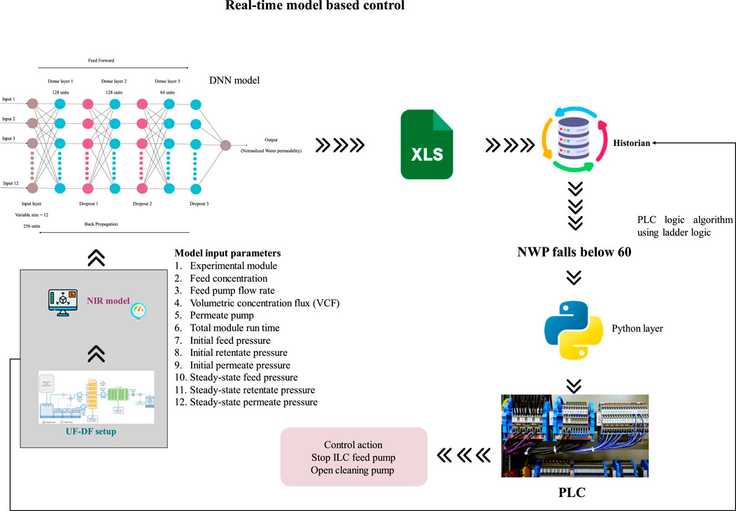
FIGURE 6. Workflow of NWP prediction and control design.

TABLE 3

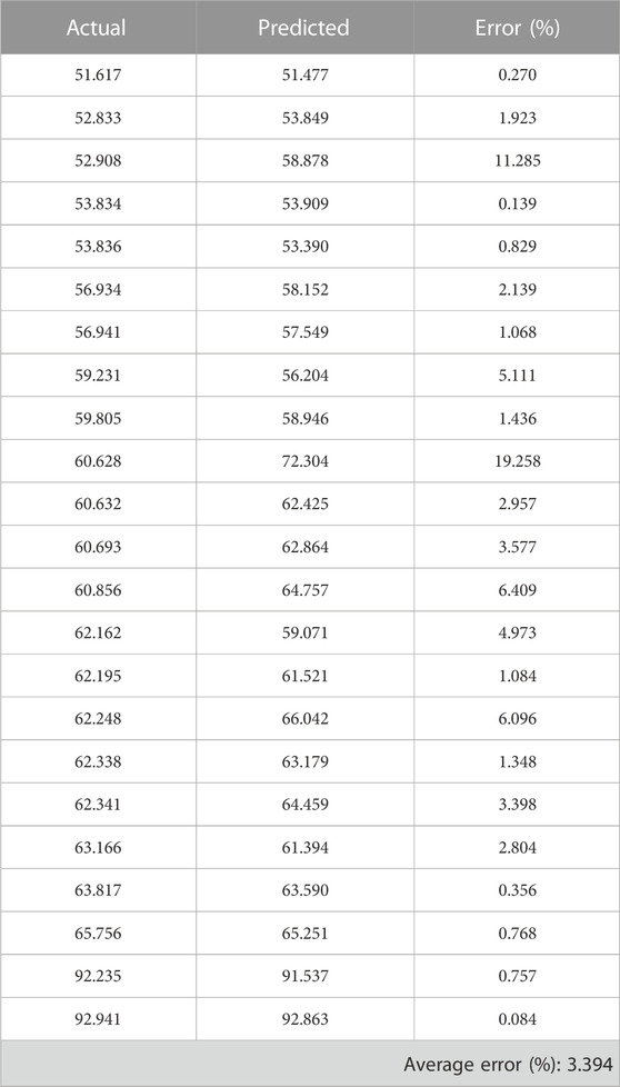
TABLE 3. Absolute values for actual NWP, predicted NWP and error percent.

FIGURE 7

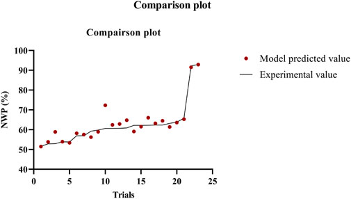
FIGURE 7. Actual vs. predicted comparison plot.

Data from the various sensors were sent to a central database on a central computer using the PLC, with the central computer also having the outlined Python script. The Python layer was utilized to input data, and it also facilitated manual input feeding for the VCF and module parameters utilized in the current process. The input feeding process activated the model, resulting in the forecasting of NWP at different randomized time intervals/experimental setups. The results are depicted in Figure 7. The NWP parameter was stored in a list format and subsequently transmitted to the statistical control layer to ascertain the optimal control action. The NWP value is read by the statistical control layer at 5-min intervals to ascertain the appropriate control action. The statistical control layer comprises a case selection algorithm to ascertain the suitable control measure based on the NWP value. When the NWP drops 60% below, the pump centralized control action is initiated by the PLC. The PLC operated according to a logic algorithm designed for PLC systems. The PLC logic algorithm refers to a prescribed set of regulations that dictate the operational procedures of a PLC. The conventional approach for conveying these concepts involves utilizing a graphical programming language known as ladder logic. Ladder logic is a visual depiction of the logic gates and programming constructs employed to regulate PLC programmes. The present investigation involved the development of a programmable logic controller (PLC) utilizing three fundamental logic operations in ladder logic, namely, AND, OR, and NOT. The aforementioned gates amalgamate the inputs to a PLC programme, generating a solitary output. The control action involved the adjustment of three pumps (feed, permeate and cleaning buffer) activities and the solenoid valve switching. The primary adjustment entailed the cessation of feed pump operation, the actuation of the valve 1 to flow the buffer for cleaning and the actuation of the valve 2 to channel the retentate into the waste in process modules one and two. In the third module of the process, the operation of the feed and permeate pumps was suspended. Additionally, the solenoid valve 1 was switched to allow for the cleaning buffer to flow, and the actuation of the valve 2 to channel the retentate into the waste. Upon completion of the preceding operation, the programmable logic controller (PLC) activated the cleaning buffer pump linked to the cleaning buffer tank. The revolutions per minute (rpm) were predetermined for the remaining unit activities in the continuous train. The overall flow of the PLC algorithm is illustrated in Figure 8. To preserve continuity with the other procedure, the duration of the cleaning was set at 30 min. Moreover, the membrane undergoes immediate cleaning whenever the NWP value drops below 60, restoring the membrane to its initial condition within a 30-min cleaning cycle. When a new run begins, the PLC will reset all parameters to zero. The PLC also allows for user customization, which might be helpful in some circumstances.

FIGURE 8

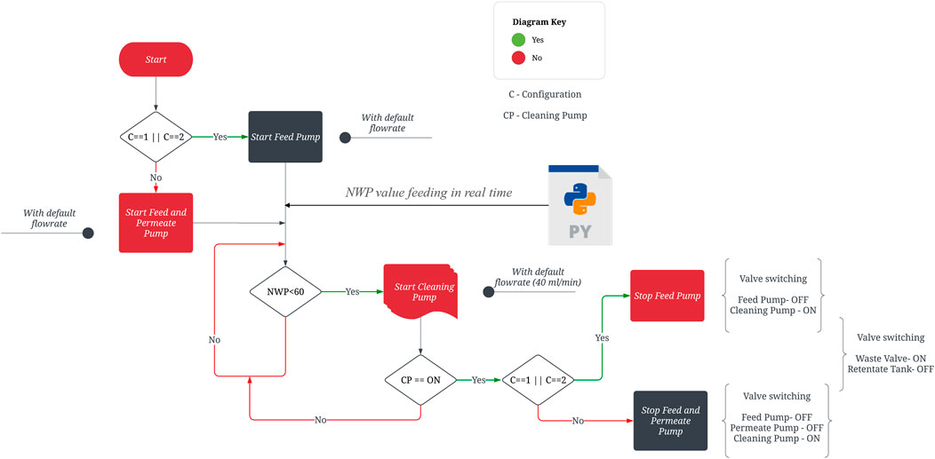
FIGURE 8. Overall workflow of the PLC algorithm.

Further elucidation regarding control action is expounded upon in the subsequent subsection through utilization of various case studies. Furthermore, the case studies serve the purpose of elucidating the performance of three distinct experimental configurations, the model’s real-time efficacy, and the suitable course of control action. The analysis of case studies facilitates comprehension of the experimental conditions appropriate for low and high monoclonal antibody concentrations. Furthermore, the utilization of case studies will aid in selecting a configuration that can effectively manage high protein concentrations while minimizing membrane cleaning frequency. Consequently, the model may be executed before commencing the experiments (preferably during the batch process), utilizing appropriate process variable values to identify optimal configuration that can operate without requiring multiple cleaning cycles. Furthermore, case studies were employed to demonstrate the intricacies of the control action. In subsequent periods, it can be integrated into a continuous process flow to establish suitable scheduling in advance and oversee the deterioration of NWP in real-time, subsequently executing requisite control measures.

3.3.1 Case study 1

In the first instance (Figure 2A), the control technique was implemented in the first process design. Five distinct trials were performed to document the performance of the model and control layer. The trials were designed randomly with different concentrations, module run time, flowrate and VCF (Figure 9). During the first trial, the model predicted an NWP value of 78, which was more than 60 and hence did not trigger a control action. In subsequent trials, the NWP was less than 60 in the fifth trial, and the PLC initiated the control method upon obtaining this result. The control strategy directed the PLC to disable the feed pump, thereby eliciting the activation of solenoid valve 1, which in turn facilitated the transition to the valve flows cleaning buffer. Furthermore, the control strategy prompted solenoid valve 2 to switch to the valve sends the retentate to waste, and subsequently activate the cleaning buffer pump. Insights into the effectiveness of the SPTFF ILC module are provided, as well as confirmation of the successful execution of the control action. When the duration of the operation ran longer (about 36.6 h), the NWP, for instance, was lower than 60. The NWP was also lower when the flowrate, VCF, and feed concentration were optimal. Module 1 can operate for 36.6 h at a VCF of around 1.7, a 20 mL/min flowrate, and a feed concentration of 33 g/L before requiring cleaning. Running the higher feed concentration of 41.7 g/L for 16.6 h at a feed flow rate of 20 mL/min and VCF of 2.3 causes a rapid decrease in the NWP value.

FIGURE 9

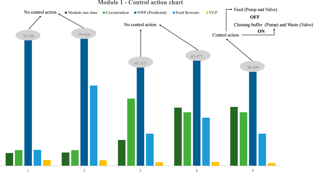
FIGURE 9. Results of model-based prediction in case study 1 for five different cycles with different feed and retentate target concentrations.

3.3.2 Case study 2

In the second scenario, the peristaltic feed pump was replaced with a quaternary pump, and the module’s control action was examined. Using quaternary pumps reduces the extent of protein exposure to mechanical stresses and air. Maintaining protein sample integrity and stability is aided by a sealed flow path and the lack of squeezing mechanisms, such as those found in peristaltic pumps. This reduces the likelihood of denaturation or aggregation. Furthermore, quaternary pumps can offer enhanced accuracy in regulating flow compared to peristaltic pumps. Accurate control of flow rate is crucial with proteins, as minor alterations in this parameter can significantly impact the outcomes of experimental investigations. Like the preceding example, five trials were done to assess the model’s real-time performance using process design 2 (Figure 10). The illustration depicts the statistical control action trigger for process design 2 (Figure 2). Nonetheless, upon analyzing the outcomes of the quaternary pump-based process design, just a few noteworthy observations were uncovered. The most significant difference is that process design 2 requires cleaning at a higher frequency than process design 1. The validity of the aforementioned assertion was determined by comparing the NWP of the membrane in process designs 1 and 2 when the concentration was 33 mg/mL and all other process parameters was kept constant (VCF is high, which is 2.7). The process design necessitated cleaning at a much shorter frequency than the previous design. The first process design can operate for 36.8 h without intermediate cleaning, whereas the second design can only operate for 16 h before requiring intermediate cleaning. However, one may argue that VCF is high for the second process design (around 15% greater). The alternative is to optimize module one in order to get the same VCF with a little reduction in overall run time.

FIGURE 10

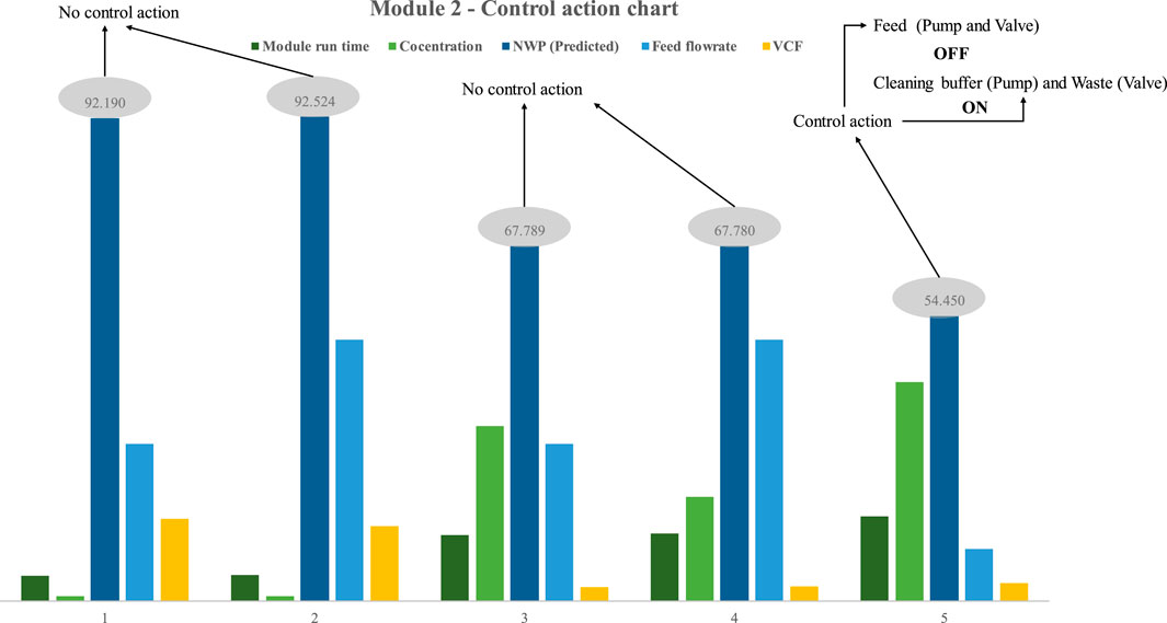
FIGURE 10. Results of model-based prediction in case study 2 for five different cycles with different feed and retentate target concentrations.

3.3.3 Case study 3

In the third instance (Figure 2C), both the feed and permeate pumps were used to operate with a more extensive concentration range. As specified, five trials with various combinations of process parameter values were utilized to assess the effectiveness of the proposed statistical control approach (Figure 11). In the first three trials, the NWP value was more than 60%, with respective values of 90.087%, 61.772%, and 63.538%. The PLC did not activate the control strategy because the NWP value sent by DCS was more than 60 percent. To verify the control action, which is the central plot of the research, parameter combinations with the highest intent were chosen to get the NWP below 60%. The recommended combination effectively reduced the NWP, with trials 4 and 5 achieving NWP reductions of 56.238 and 57.354, respectively. In a fraction of a second, the NWP values were saved in the DCS and sent to the mainframe. The PLC initiated the control operation upon receiving the signal from the DCS. Following the activation of the control action, the PLC deactivated the feed pump and permeate pump, thereby inducing the initiation of solenoid valve 1, which subsequently facilitated the transition to the valve flows cleaning buffer. Additionally, the control methodology prompted solenoid valve 2 to transition to the valve that conveys the retentate to waste, and subsequently activate the cleaning buffer pump. PLC let the cleaning buffer pump operate for 30 min to return the membrane to its starting condition. Except for the effective execution of the control strategy for process design 3, few notable findings were made. Compared to using a single pump, either peristatic or quaternary, the efficiency of using both the feed and permeate pumps is much greater. The NWP of trial three was 61 after 21 h of operation with a feed concentration of 20 mL/min, a feed flowrate of 30 mL/min, a permeate flowrate of 27.7 mL/min, and a VCF of 13. Even though the overall runtime was lengthy in the first two cases, the operation flowrate was slower. In the third case, however, installing a permeate pump enables a more significant flow rate, which is challenging to maintain in the other two circumstances. During the fifth trial, the NWP was 56, the feed flow rate was 30 mL/min, the permeate flow rate was 19 mL/min, the feed concentration was 26 mg/mL, the VCF was 2.7, and the total run time was 28 h.

FIGURE 11

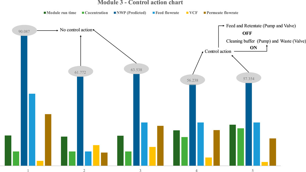
FIGURE 11. Results of model-based prediction in case study 3 for five different cycles with different feed and retentate target concentrations. The results demonstrate that the module can function for 28 h at a high concentration and flow rate without requiring any interim cleaning, thereby enabling the design of the process to cope with the other two modules in terms of concentration, feed flow rate, and overall run time. In addition, Process Design 3 is the most optimal since it allows for a high operating flow rate within a reasonable total run time. The user can choose the three architectures presented here according to their needs. The developed DNN model’s efficacy across all scenarios was demonstrated with the help of case studies. Process Design 3 is preferable for a continuous process since it is easier to deploy in real-time and apply control strategies.

4 Conclusion

A deep neural network model has been developed to predict the NWP in real-time in single-pass tangential flow filtration of mAbs. The model utilizes process parameters, including pressure and feed concentrations via inline sensors and a spectroscopy-coupled data model, and is used to schedule membrane cleaning steps at the optimal time when the NWP drops below 60%. Using SCADA and PLC, a distributed control system has been developed to integrate the monitoring sensors and control elements, such as the NIRS sensor for concentration monitoring, the DNN model for NWP prediction, weighing balances, pressure sensors, pumps, and valves. The model was tested in real-time, and the NWP was predicted within <5% error in three independent test cases. In general, a reduction in flux can aid in comprehending the contemporaneous decrease in NWP. Nevertheless, determining the absolute drop via a primary calibration curve of flux versus NWP is challenging. The decline of NWP is contingent upon additional variables such as feed flowrate and feed concentration. A mere calibration remedy would not yield precise results. Utilizing the deep learning methodology enables the comprehensive consideration of all pertinent variables that may exert a direct or indirect impact on the NWP. Thus, the constructed framework was utilized to forecast accurate NWP during the process without interrupting the process to conduct NWP measurement experiments. This work leverages PAT and DL to enable automated, integrated, and well-controlled STPFF operations. The approach is consistent with the US FDA’s guidance on Quality by Design (QbD), as it utilizes product and process understanding to adjust process parameters to consistently meet CQA targets in biopharmaceutical manufacturing processes in the final formulation step.

Data availability statement

The raw data supporting the conclusion of this article will be made available by the authors, without undue reservation.

Author contributions

NJ and GT performed the experiments. NJ contributed to development of the model. NJ and GT wrote the first draft. AR supervised the project, got the funding and reviewed and edited the final manuscript. All authors contributed to the article and approved the submitted version.

Acknowledgments

We would like to acknowledge funding support from the Department of Biotechnology, Ministry of Science and Technology (Number BT/COE/34/SP15097/2015). We would like to declare that they do not have any conflict of interest.

Conflict of interest

The authors declare that the research was conducted in the absence of any commercial or financial relationships that could be construed as a potential conflict of interest.

Publisher’s note

All claims expressed in this article are solely those of the authors and do not necessarily represent those of their affiliated organizations, or those of the publisher, the editors and the reviewers. Any product that may be evaluated in this article, or claim that may be made by its manufacturer, is not guaranteed or endorsed by the publisher.

References

Adib, H., Raisi, A., and Salari, B. (2019). Support vector machine-based modeling of grafting hyperbranched polyethylene glycol on polyethersulfone ultrafiltration membrane for separation of oil–water emulsion. Res. Chem. Intermed. 45, 5725–5743. doi:10.1007/s11164-019-03931-z

CrossRef Full Text | Google Scholar

Barello, M., Manca, D., Patel, R., and Mujtaba, I. M. (2014). Neural network based correlation for estimating water permeability constant in RO desalination process under fouling. Desalination 345, 101–111. doi:10.1016/j.desal.2014.04.016

CrossRef Full Text | Google Scholar

Chakrabarti, A., and Ghosh, J. K. (2011). AIC, BIC and recent advances in model selection. Philosophy statistics 7, 583–605. doi:10.1016/B978-0-444-51862-0.50018-6

CrossRef Full Text | Google Scholar

Chew, C. M., Aroua, M. K., and Hussain, M. A. (2017). A practical hybrid modelling approach for the prediction of potential fouling parameters in ultrafiltration membrane water treatment plant. J. Industrial Eng. Chem. 45, 145–155. doi:10.1016/j.jiec.2016.09.017

CrossRef Full Text | Google Scholar

Chhabra, H., Jesubalan, N. G., and Rathore, A. S. (2023). Soft sensor based rapid detection of trace chlorine dioxide (ClO2) concentration in water. Water Res. 242, 120231. doi:10.1016/j.watres.2023.120231

PubMed Abstract | CrossRef Full Text | Google Scholar

Cho, J.-S., Kim, H., Choi, J.-S., Lee, S., Hwang, T.-M., Oh, H., et al. (2010). Prediction of reverse osmosis membrane fouling due to scale formation in the presence of dissolved organic matters using genetic programming. Desalination Water Treat. 15, 121–128. doi:10.5004/dwt.2010.1675

CrossRef Full Text | Google Scholar

Cho, S. J., and Tropsha, A. (1995). Cross-validated R2-guided region selection for comparative molecular field analysis: A simple method to achieve consistent results. J. Med. Chem. 38 (7), 1060–1066. doi:10.1021/jm00007a003

PubMed Abstract | CrossRef Full Text | Google Scholar

Dornier, M., Decloux, M., Trystram, G., and Lebert, A. (1995). Dynamic modeling of crossflow microfiltration using neural networks. J. Membr. Sci. 98, 263–273. doi:10.1016/0376-7388(94)00195-5

CrossRef Full Text | Google Scholar

Eğrioğlu, E., Aladağ, Ç. H., and Günay, S. (2008). A new model selection strategy in artificial neural networks. Appl. Math. Comput. 195 (2), 591–597. doi:10.1016/j.amc.2007.05.005

CrossRef Full Text | Google Scholar

Fazeli, H., Soleimani, R., Ahmadi, M.-A., Badrnezhad, R., and Mohammadi, A. H. (2013). Experimental study and modeling of ultrafiltration of refinery effluents using a hybrid intelligent approach. Energy fuels. 27, 3523–3537. doi:10.1021/ef400179b

CrossRef Full Text | Google Scholar

Frazier, P. I. (2018a). A tutorial on Bayesian optimization. arXiv preprint arXiv:1807.02811.

Google Scholar

Frazier, P. I. (2018b). “Bayesian optimization,” in Recent advances in optimization and modeling of contemporary problems (Informs), 255–278.

CrossRef Full Text | Google Scholar

Hodson, T. O. (2022). Root-mean-square error (RMSE) or mean absolute error (MAE): When to use them or not. Geosci. Model Dev. 15 (14), 5481–5487. doi:10.5194/gmd-15-5481-2022

CrossRef Full Text | Google Scholar

Jabra, M. G., Lipinski, A. M., and Zydney, A. L. (2021). Single pass tangential flow filtration (SPTFF) of monoclonal antibodies: Experimental studies and theoretical analysis. J. Membr. Sci. 637, 119606. doi:10.1016/j.memsci.2021.119606

CrossRef Full Text | Google Scholar

Jawad, J., Hawari, A. H., and Javaid Zaidi, S. (2021). Artificial neural network modeling of wastewater treatment and desalination using membrane processes: A review. Chem. Eng. J. 419, 129540. doi:10.1016/j.cej.2021.129540

CrossRef Full Text | Google Scholar

Jerez, M. J. O., Pasos, C. A. V., and Mejía, E. F. (2008). Mathematical models of membrane fouling in cross-flow micro-filtration. Ing. Investig. 28, 123–132. doi:10.15446/ing.investig.v28n1.14876

CrossRef Full Text | Google Scholar

Kaiser, J., Krarup, J., Hansen, E. B., Pinelo, M., and Krühne, U. (2022). Defining the optimal operating conditions and configuration of a single-pass tangential flow filtration (SPTFF) system via CFD modelling. Sep. Purif. Technol. 290, 120776. doi:10.1016/j.seppur.2022.120776

CrossRef Full Text | Google Scholar

Kateja, N., Agarwal, H., Saraswat, A., Bhat, M., and Rathore, A. S. (2016). Continuous precipitation of process related impurities from clarified cell culture supernatant using a novel coiled flow inversion reactor (CFIR). Biotechnol. J. 11 (10), 1320–1331. doi:10.1002/biot.201600271

PubMed Abstract | CrossRef Full Text | Google Scholar

Khayet, M., and Cojocaru, C. (2013). Artificial neural network model for desalination by sweeping gas membrane distillation. Desalination, New Dir. Desalination 308, 102–110. doi:10.1016/j.desal.2012.06.023

CrossRef Full Text | Google Scholar

Kim, S. J., Oh, S., Lee, Y. G., Jeon, M. G., Kim, I. S., and Kim, J. H. (2009). A control methodology for the feed water temperature to optimize SWRO desalination process using genetic programming. Desalination 247, 190–199. doi:10.1016/j.desal.2008.12.024

CrossRef Full Text | Google Scholar

Koehrsen, W. (2018). Automated machine learning hyperparameter tuning in Python. Medium. Available at: https://towardsdatascience.com/automated-machine-learning-hyperparameter-tuning-in-python-dfda59b72f8a (Accessed July 4, 2018).

Google Scholar

Krippl, M., Kargl, T., Duerkop, M., and Dürauer, A. (2021). Hybrid modeling reduces experimental effort to predict performance of serial and parallel single-pass tangential flow filtration. Sep. Purif. Technol. 276, 119277. doi:10.1016/j.seppur.2021.119277

CrossRef Full Text | Google Scholar

Laud, P. W., and Ibrahim, J. G. (1995). Predictive model selection. J. R. Stat. Soc. Ser. B Methodol. 57 (1), 247–262. doi:10.1111/j.2517-6161.1995.tb02028.x

CrossRef Full Text | Google Scholar

Li, M., Ebel, B., Chauchard, F., Guédon, E., and Marc, A. (2018). Parallel comparison of in situ Raman and NIR spectroscopies to simultaneously measure multiple variables toward real-time monitoring of CHO cell bioreactor cultures. Biochem. Eng. J. 137, 205–213. doi:10.1016/j.bej.2018.06.005

CrossRef Full Text | Google Scholar

Madaeni, S. S., and Kurdian, A. R. (2011). Fuzzy modeling and hybrid genetic algorithm optimization of virus removal from water using microfiltration membrane. Chem. Eng. Res. Des. 89, 456–470. doi:10.1016/j.cherd.2010.07.009

CrossRef Full Text | Google Scholar

Masum, M., Shahriar, H., Haddad, H., Faruk, M. J. H., Valero, M., Khan, M. A., et al. (2021). “Bayesian hyperparameter optimization for deep neural network-based network intrusion detection,” in 2021 IEEE International Conference on Big Data (Big Data), Orlando, FL, USA, 15-18 December 2021, 5413–5419. doi:10.1109/BigData52589.2021.9671576

CrossRef Full Text | Google Scholar

Montavon, G., Samek, W., and Müller, K. R. (2018). Methods for interpreting and understanding deep neural networks. Digit. signal Process. 73, 1–15. doi:10.1016/j.dsp.2017.10.011

CrossRef Full Text | Google Scholar

Natarajan, P., Moghadam, R., and Jagannathan, S. (2021). Online deep neural network-based feedback control of a Lutein bioprocess. J. Process Control 98, 41–51. doi:10.1016/j.jprocont.2020.11.011

CrossRef Full Text | Google Scholar

Nejad, A. R. S., Ghaedi, A. M., Madaeni, S. S., Baneshi, M. M., Vafaei, A., Emadzadeh, D., et al. (2019). Development of intelligent system models for prediction of licorice concentration during nanofiltration/reverse osmosis process. Desalination Water Treat. 145, 83–95. doi:10.5004/dwt.2019.23731

CrossRef Full Text | Google Scholar

Nikita, S., Thakur, G., Jesubalan, N. G., Kulkarni, A., Yezhuvath, V. B., and Rathore, A. S. (2022). AI-ML applications in bioprocessing: ML as an enabler of real time quality prediction in continuous manufacturing of mAbs. Comput. Chem. Eng. 164, 107896. doi:10.1016/j.compchemeng.2022.107896

CrossRef Full Text | Google Scholar

Parhi, R., and Nowak, R. D. (2020). The role of neural network activation functions. IEEE Signal Process. Lett. 27, 1779–1783. doi:10.1109/lsp.2020.3027517

CrossRef Full Text | Google Scholar

Pirrung, S. M., van der Wielen, L. A. M., van Beckhoven, R. F. W. C., van de Sandt, E. J. A. X., Eppink, M. H. M., and Ottens, M. (2017). Optimization of biopharmaceutical downstream processes supported by mechanistic models and artificial neural networks. Biotechnol. Prog. 33 (3), 696–707. doi:10.1002/btpr.2435

PubMed Abstract | CrossRef Full Text | Google Scholar

Quinino, R. C., Reis, E. A., and Bessegato, L. F. (2013). Using the coefficient of determination R2 to test the significance of multiple linear regression. Teach. Stat. 35 (2), 84–88. doi:10.1111/j.1467-9639.2012.00525.x

CrossRef Full Text | Google Scholar

Rahimzadeh, A., Ashtiani, F. Z., and Okhovat, A. (2016). Application of adaptive neuro-fuzzy inference system as a reliable approach for prediction of oily wastewater microfiltration permeate volume. J. Environ. Chem. Eng. 4, 576–584. doi:10.1016/j.jece.2015.12.011

CrossRef Full Text | Google Scholar

Rahmanian, B., Pakizeh, M., Mansoori, S. A. A., and Abedini, R. (2011). Application of experimental design approach and artificial neural network (ANN) for the determination of potential micellar-enhanced ultrafiltration process. J. Hazard. Mater. 187, 67–74. doi:10.1016/j.jhazmat.2010.11.135

PubMed Abstract | CrossRef Full Text | Google Scholar

Rahmanian, B., Pakizeh, M., Mansoori, S. A. A., Esfandyari, M., Jafari, D., Maddah, H., et al. (2012). Prediction of MEUF process performance using artificial neural networks and ANFIS approaches. J. Taiwan Inst. Chem. Eng. 43, 558–565. doi:10.1016/j.jtice.2012.01.002

CrossRef Full Text | Google Scholar

Razavi, M. A., Mortazavi, A., and Mousavi, M. (2003). Dynamic modelling of milk ultrafiltration by artificial neural network. J. Membr. Sci. 220, 47–58. doi:10.1016/S0376-7388(03)00211-4

CrossRef Full Text | Google Scholar

Salehi, F., and Razavi, S. M. A. (2012). Dynamic modeling of flux and total hydraulic resistance in nanofiltration treatment of regeneration waste brine using artificial neural networks. Desalination Water Treat. 41, 95–104. doi:10.1080/19443994.2012.664683

CrossRef Full Text | Google Scholar

Salehi, F., and Razavi, S. M. A. (2016). Modeling of waste brine nanofiltration process using artificial neural network and adaptive neuro-fuzzy inference system. Desalination Water Treat. 57, 14369–14378. doi:10.1080/19443994.2015.1063087

CrossRef Full Text | Google Scholar

Shcherbakov, M. V., Brebels, A., Shcherbakova, N. L., Tyukov, A. P., Janovsky, T. A., and Kamaev, V. A. (2013). A survey of forecast error measures. World Appl. Sci. J. 24 (24), 171–176. doi:10.5829/idosi.wasj.2013.24.itmies.80032

CrossRef Full Text | Google Scholar

Shokrkar, H., Salahi, A., Kasiri, N., and Mohammadi, T. (2012). Prediction of permeation flux decline during MF of oily wastewater using genetic programming. Chem. Eng. Res. Des. 90, 846–853. doi:10.1016/j.cherd.2011.10.002

CrossRef Full Text | Google Scholar

Srinidhi, C. L., Ciga, O., and Martel, A. L. (2021). Deep neural network models for computational histopathology: A survey. Med. Image Anal. 67, 101813. doi:10.1016/j.media.2020.101813

PubMed Abstract | CrossRef Full Text | Google Scholar

Stoller, M., and Serrão Mendes, R. (2017). Advanced control system for membrane processes based on the boundary flux model. Sep. Purif. Technol. 175, 527–535. doi:10.1016/j.seppur.2016.09.049

CrossRef Full Text | Google Scholar

Thakur, G., Masampally, V., Kulkarni, A., and Rathore, A. S. (2022). Process analytical technology (PAT) implementation for membrane operations in continuous manufacturing of mAbs: Model-based control of single-pass tangential flow ultrafiltration. AAPS J. 24, 83. doi:10.1208/s12248-022-00731-z

PubMed Abstract | CrossRef Full Text | Google Scholar

Wang, L., Zhou, X., Zhu, X., Dong, Z., and Guo, W. (2016). Estimation of biomass in wheat using random forest regression algorithm and remote sensing data. Crop J. 4, 212–219. doi:10.1016/j.cj.2016.01.008

CrossRef Full Text | Google Scholar

West, S. G., Taylor, A. B., and Wu, W. (2012). “Model fit and model selection in structural equation modeling,” in Handbook of structural equation modeling (New York, NY: The Guilford Press), 209–231.

Google Scholar

Yegnanarayana, B. (2009). Artificial neural networks. New Delhi, India: PHI Learning Pvt. Ltd.

Google Scholar

Zou, J., Han, Y., and So, S.-S. (2009). “Overview of artificial neural networks,” in Artificial Neural Networks: Methods and Applications. Editor D. J. Livingstone (Totowa, NJ: Humana Press), 14–22. Available at: https://doi.org/10.1007/978-1-60327-101-1_2.

Google Scholar