A feasible path-based branch and bound algorithm for strongly nonconvex MINLP problems

In this paper, a feasible path-based branch and bound (B&B) algorithm is proposed to solve mixed-integer nonlinear programming problems with highly nonconvex nature through integration of the previously proposed hybrid feasible-path optimisation algorithm and the branch and bound method. The main advantage of this novel algorithm is that our previously proposed hybrid steady-state and time-relaxation-based optimisation algorithm is employed to solve a nonlinear programming (NLP) subproblem at each node during B&B. The solution from a parent node in B&B is used to initialize the NLP subproblems at the child nodes to improve computational efficiency. This approach allows circumventing complex initialisation procedure and overcoming difficulties in convergence of process simulation. The capability of the proposed algorithm is illustrated by several process synthesis and intensification problems using rigorous models.

1 Introduction

Many optimisation problems in the field of chemical engineering are usually modeled as mixed-integer nonlinear programming (MINLP) problems. Typical examples include process synthesis problems, design and scheduling of batch processes, molecular design and integration of process design and control. MINLP optimisation problems involve integer or discrete variables in addition to continuous variables. Continuous variables are used to optimize operating conditions such as input and output flow rates of an individual unit, unit operating pressure and temperature, reaction conversion, and product recoveries. Integer variables can be used to make discrete decisions, e.g., selection of process equipment or assignment of tasks. It is also possible to introduce discrete quantities, such as number of trays in a distillation column (Kronqvist et al., 2018). The coupling of the integer domain and the continuous domain, as well as their associated nonlinearities, makes MINLP problems extremely difficult to solve theoretically, algorithmically and computationally (Floudas, 2009).

In general, MINLP problems can be divided into two classes - convex MINLP problems and nonconvex MINLP problems. A convex MINLP problem is defined as such when the discrete binaries are relaxed as continuous variables, the resulting NLP problem is convex (Trespalacios and Grossmann, 2014). A number of deterministic algorithms for solving convex MINLP problems have been proposed, primarily based on two optimisation methods, the branch and bound method and the MILP decomposition method (Kronqvist and Lundell, 2019). The main idea of the branch and bound (B&B) method (Gupta and Ravindran, 1985) is used in most of the existing MINLP deterministic solvers. B&B builds up a search tree to implicitly enumerate possible candidate solutions for a given problem, using pruning rules to eliminate search regions where a better solution cannot be found (Morrison et al., 2016). When a tree search is performed, the integer variables are successively fixed at the corresponding nodes of the tree, yielding relaxed NLP subproblems. It is only attractive if NLP subproblems are inexpensive to solve, or only a few of them need to be solved. In contrast to B&B, the main idea of the MILP decomposition approaches is to iteratively construct a MILP approximation by successive linearization of nonlinear constraints without using a search tree. Algorithms include outer approximation (OA) (Viswanathan and Grossmann, 1990), the extended cutting plane method (ECP) (Westerlund and Pettersson, 1995), extended supporting hyperplane (ESH) (Kronqvist et al., 2015) and generalised bender decomposition (GBD) (Geoffrion, 1972). Apart from the above algorithms, Raman and Grossmann (1994) brought up an alternative representation of MINLP—Generalised Disjunctive Programming (GDP), which involves Boolean and continuous variables that are specified in algebraic constraints, disjunctions and logic propositions. These GDP problems can be solved by dedicated solution algorithms such as logic-based OA (Türkay and Grossmann, 1996) and GDP B&B (Lee and Grossmann, 2000).

Although both types of MINLP problems are NP-hard in general, nonconvex MINLP problems are typically much harder to solve than convex MINLP problems (Burer and Letchford, 2012). This is due to nonconvexities of integer variables as well as nonconvex functions in the objective function and/or constraints in nonconvex MINLP problems. Even if the integrality requirements are relaxed, the feasible region may continue to be nonconvex (KILINÇ and SAHINIDIS, 2017) as nonconvex constraints are typically required for accurate modeling of many real-world problems, particularly in chemical engineering. The nature of nonconvexities implies the potential existence of multiple local optimal solutions. As a result, a local optimal solution for nonconvex problems is frequently obtained, whilst the global optimal solution for convex MINLP problems is guaranteed. In response to the increased number of applications, a variety of global optimization algorithms for nonconvex MINLP problems have been developed, which can be classified as deterministic or stochastic depending on their convergence features.

The most common global deterministic method to solve nonconvex MINLP problems is spatial B&B (McCormick, 1976). It extends the scope of traditional branch and bound algorithm to solving problems for which the feasible region of continuous variables is divided and the lower bound and upper bound are compared for fathoming each subregion. Two major algorithms derived from spatial B&B make a step forward for finding the exact solution of nonconvex MINLP problems. One is the branch and reduce algorithm (Ryoo and Sahinidis, 1996), while the other is α-branch and bound algorithm (Androulakis et al., 1995). The branch and reduce algorithm is based on the idea that convex underestimating NLPs can be constructed for the nonconvex relaxations by evolutionary subdivision of the search region. It is commonly conducted on LP relaxations rather than more complex convex programming relaxations (Burer and Letchford, 2012). The α-branch and bound algorithm relied on the idea of modifying the Hessian matrix of the Lagrangian function in nonconvex NLP problems to yield a convex relaxation. Although these two methods can theoretically guarantee global optimality, they are often very computational demanding, due to the generation of a huge global search tree, which may prevent the method to find an optimal solution within a reasonable time (Burre et al., 2022). They often fail to find a feasible solution for large-scale highly nonconvex MINLP problems.

Different from deterministic methods which requires the knowledge about the problem structure, stochastic methods treat the problems to be optimised as a black box. They include simulated annealing, genetic algorithm, and clustering methods. Their robustness and ease of implementation make them commonly adopted to solve difficult optimisation problems. However, there is no guarantee that such algorithms can approach optimality. Moreover, stochastic algorithms require a large number of fitness evaluations due to the combinatorial nature of sampling multidimensional space, leading to long computational time. For example, one simulation run for a pressure swing distillation case (Battisti et al., 2019) using simulated annealing algorithm can be up to 1 h. Multiple runs have to be conducted with difference parameters in order to find the closest proximity to the global optimum. This may get much worse for solving MINLP problems since the presence of integer variables results in a combinatorial explosion of solutions. That is why their use for solving MINLP problems remains limited (Munawar et al., 2011).

Concerning the robustness of NLP solvers and the fact that globally optimising MINLP models for large-scale problems using the methods described above can be very computationally expensive, solvers such as DICOPT (Viswanathan and Grossmann, 1990) and SBB are used to solve large-scale nonconvex MINLP problems, despite the fact that these methods rely on convexity assumptions (Grossmann, 2012). In the past few decades, the aforementioned algorithms have been applied to a wide range of problems in the field of process systems engineering. Some modified OA methods have been applied to the simultaneous optimisation of heat integration network (Yee and Grossmann, 1990), distillation column synthesis (Farkas et al., 2008), and the optimisation of an integrated five-level Supply Chain (Amjadian and Gharaei, 2021). Logic based OA algorithm has been applied to the optimal design of reactive distillation columns (Jackson and Grossmann, 2001). Branch and bound method has also been applied to identify energy-efficient distillation configurations for multicomponent separations (Tumbalam Gooty, 2019) and the optimal design of catalytic distillation (Liñán et al., 2021). However, as pointed out by Grossmann (2012), the key of successfully solving MINLP problems is to solve NLP subproblems and the convergence of NLP subproblems must require the supply of good initial points and accurate derivative information. In other words, the solvers such as DICOPT and SBB often fail if a good initial point is not supplied.

Another way to improve the convergence of NLP subproblems is to make systematic use of solutions generated from previous NLP subproblems, which has been addressed in our previous work (Ma and Li, 2022). The homotopy continuation method was employed to improve the convergence and efficiency of solving the NLP subproblems at each node through constructing a homotopy path using the solution obtained from its parent node. However, two specialized initialisation strategies were designed to generate a feasible solution for the relaxed synthesis problems at the root node, and this feasible solution was then used to initialise the proposed homotopy continuation enhanced branch and bound algorithms. This implies that “good” initial points are required. More importantly, HCBB method may fail if the homotopy path is discontinuous. In addition, this HCBB method is difficult to be used to solve MINLP problems with many constraints implicitly indicated in a process simulator such as Aspen Custom Modeller (ACM).

It is not difficult to notice that two of the main applications of MINLP in chemical engineering are process synthesis and intensification. Process intensification has been receiving increased attention because of its potential to obtain process improvement and meet the increasing demands for sustainable production (Lutze et al., 2010). The reduction of equipment size, higher energy efficiency, reduction in capital cost and safer operation can be achieved in the intensified process unit. In particular, the diving wall column (DWC) is a practical implementation of a fully thermally coupled distillation column in which mixtures of three or more components can be separated into high purity products (Dejanovic et al., 2010). The objective of process synthesis is to select the best process flowsheet among numerous alternatives. The selection of the optimal configuration for the separation of a multicomponent mixture is one of the prevailing problems for superstructure optimisation-based synthesis problems. In the optimisation of DWC column and distillation sequence synthesis problem, many methods presented in the literature are based on short-cut models. They may show good convergence performance and are less computationally intensive, but the solutions are often impractical due to the simplified assumptions. Thus, unit rigorous models are required to be incorporated which leads to highly nonconvexity and nonlinearities that translate to pronounced computational difficulties in achieving convergence by using the existing algorithms.

To overcome the difficulties of the existing optimisation methods in solving highly nonconvex MINLP problems, we develop a new solution approach - a feasible path-based branch and bound algorithm in this paper. Like conventional branch and bound method, a search tree needs to be created. The key difference is that a hybrid feasible path-based optimisation framework is applied for solving the relaxed NLP subproblems at each node. With this combination, our new proposed MINLP algorithm possesses the following superiorities:

• No tailor-made initialisation procedure is required. Initial points can be chosen randomly, and convergence can be guaranteed.

• It overcomes the convergence difficulties when highly nonconvex constraints are incorporated in the mathematical models in the equation-oriented environment, e.g., thermodynamic equilibrium models and MESH equations for distillation.

• As the mathematical models are implemented in the process simulator, which has physical property database, the calculation of physical properties can be repeatedly carried out. No simplified assumptions have to be made on the physical properties such as ideal gas or liquid phase behaviour. Thus, there is no compromise on the model accuracy.

Several examples involving DWC optimisation and distillation sequence synthesis are solved to illustrate the capability of the proposed new algorithm. The computational results demonstrate that a similar configuration of DWC and very close TAC are obtained for Example 1 compared to the results in the literature. For Examples 2 and 3, at least 15% energy reduction can be achieved, compared to the results in the literature. For distillation sequence synthesis problems, the optimum solutions can be found within 1,723 CPU s for a ternary mixture and 2,470 CPU s for a quaternary mixture. Note that the main purpose of this work is to demonstrate the feasibility and superiority of the proposed algorithm by solving several examples. Hence, we do not conduct comprehensive evaluation of the proposed algorithm, which will be our future publication.

The rest of this paper is structured as follows: The MINLP problem to be solved is introduced first. The FPBB algorithm is then be explained in detail. After that, several examples including dividing wall column optimisation and the synthesis of distillation sequences are presented to illustrate the effectiveness of our novel algorithm. Finally, we conclude our work with some insights and future endeavour.

2 Problem statement

The large-scale highly nonconvex MINLP problem usually has the following general form:

$\begin{array}{l}\underset{\mathbf{x},\mathbf{y}}{\min }f\left(\mathbf{x},\mathbf{y}\right)\\ s.t.\mathbf{h}\left(\mathbf{x},\mathbf{y}\right)=0\\ \mathbf{g}\left(\mathbf{x},\mathbf{y}\right)\le 0\\ \mathbf{x}\in \mathit{X}\subseteq R^n,\mathbf{y}\in Z^s\text{integer}\end{array}(\mathrm{P1})$

where $\mathbf{x}$ is a vector of continuous variables with $n$ dimension, and y is a set of integer variables; $f\left(\mathbf{x},\mathbf{y}\right)$ usually represents the objective function such as total annualised cost (TAC); $\mathbf{h}\left(\mathbf{x},\mathbf{y}\right)=0$ are equality constraints such as material and energy balances, and equilibrium relationships; $\mathbf{g}\left(\mathbf{x},\mathbf{y}\right)\le 0$ are inequality constraints such as product specifications and minimum temperature difference requirements in the heat exchangers. When we constrain the set of integer variables to binary variables without loss of generality (Floudas, 2009), the original MINLP problem can be formulated as below:

$\begin{array}{l}\underset{\mathbf{x},\mathbf{y}}{\min }f\left(\mathbf{x},\mathbf{y}\right)\\ s.t.\mathbf{h}\left(\mathbf{x},\mathbf{y}\right)=0\\ \mathbf{g}\left(\mathbf{x},\mathbf{y}\right)\le 0\\ \mathbf{x}\in \mathit{X}\subseteq R^n,\mathbf{y}\in {\left\{\mathrm{0,1}\right\}}^s\end{array}(\mathrm{P2})$

where $\mathbf{y}$ now is a vector of 0–1 variables with dimension $s$, for instance, existence of a process unit $\left(y_i=1\right)$ or nonexistence $\left(y_i=0\right)$. In this paper, $f\left(\cdot \right),\mathbf{g}\left(\cdot \right)$ and $\mathbf{h}\left(\cdot \right)$ are assumed to be smooth, twice differentiable and noncovex with respect to $\mathit{x}$.

The objective of this work is to develop a novel branch and bound algorithm called feasible path-based branch and bound algorithm coupled hybrid steady-state and time-relaxation-based algorithm (denoted as FPBB) to solve the above stated problem P2.

3 Feasible path-based branch and bound algorithm

The standard nonlinear B&B algorithm (SBB) for an MINLP problem is a combination of the branch and bound method with a selected NLP solver. Since an NLP subproblem is required to solve at each B&B node, the performance of SBB on the MINLP problems mainly depends on how to solve the NLP subproblems reliably. When feasible solutions exist for NLP subproblems, failing to solve them can severely impede the performance of MINLP algorithms (Flores-Tlacuahuac and Biegler, 2007). To solve large-scale highly nonconvex NLP subproblems (e.g., distillation column optimization based on MESH equations) reliably, we employ the hybrid feasible path optimisation algorithm developed previously in which an NLP subproblem is decomposed into two layers, as it has demonstrated its capabilities for solving large-scale strongly nonconvex nonlinear optimisation problems. In the sequel, we introduce the feasible path algorithm in detail.

For clarity, some notations need to be introduced first. The active nodes set that includes the remaining nodes to be explored in the B&B is denoted as $\zeta$. During B&B, for example, at node $n_i$, some of binary variables are fixed, while some remain relaxed. Before solving the subproblem at the node n_i, the fixed set of binary variables is denoted as ${\mathit{y}}_F^i$, the relaxed set is denoted as ${\mathit{y}}_R^i$. After solving the subproblem.

Solving the subproblem, the fixed set is still the same as ${\mathit{y}}_F^i$, however, the relaxed set is changed to ${\mathit{y}}_R^{i*}$ with determined optimal values. ${\stackrel{\sim }{f}}_i^{*}$ is used to denote the optimal objective value of the NLP subproblem at node ${\mathit{n}}_{\mathit{i}}$, and ${\stackrel{\sim }{f}}^{ub}$ is used to denote the upper bound of the MINLP problem. At a node $n_i$, the NLP subproblem is then defined as follows,

$\begin{array}{l}\underset{\mathbf{x},{\mathit{y}}_R^i}{\min }f\left(\mathbf{x},{\mathit{y}}_R^i\right)\\ s.t.\mathbf{h}\left(\mathbf{x},{\mathit{y}}_R^i\right)=0\\ \mathbf{g}\left(\mathbf{x},{\mathit{y}}_R^i\right)\le 0\\ \mathbf{x}\in \mathit{X}\subseteq R^n,{\mathit{y}}_R^i\in {\left(\mathrm{0,1}\right)}^q\end{array}(\mathrm{P3})$

Where ${\mathit{y}}_{\mathit{R}}^{\mathit{i}}$ is the set of relaxed binary variables with a dimension of $\mathit{q}$ at node ${\mathit{n}}_{\mathit{i}}$.

3.1 Hybrid feasible path optimisation algorithm

In problem P3, equality constrains can be divided to two groups - one group contains the unit operation models (e.g., mass and energy balances, equilibrium relationships), stream connections and economic evaluation models, denoted as ${\mathbf{h}}_1$, while the others are denoted as ${\mathbf{h}}_2$. Then problem P3 is changed to below form:

$\begin{array}{l}\underset{\mathbf{x},{\mathit{y}}_R^i}{\min }f\left(\mathbf{x},{\mathit{y}}_R^i\right)\\ s.t.{\mathbf{h}}_1\left(\mathbf{x},{\mathit{y}}_R^i\right)=0\\ {\mathbf{h}}_2\left(\mathbf{x},{\mathit{y}}_R^i\right)=0\\ \mathbf{g}\left(\mathbf{x},{\mathit{y}}_R^i\right)\le 0\\ \mathbf{x}\in \mathit{X}\subseteq R^n,{\mathit{y}}_R^i\in {\left\{\mathrm{0,1}\right\}}^q\end{array}(\mathrm{P4})$

If partitioning continuous variables $\mathbf{x}$ in problem P3 into two sets - independent variables ${\mathbf{x}}_{\mathrm{I}}$ and dependent variables ${\mathbf{x}}_{\mathrm{D}}$, and the dimension of ${\mathbf{x}}_{\mathrm{D}}$ is equal to that of ${\mathbf{h}}_1$. As ${\mathbf{x}}_{\mathrm{D}}$ can be expressed using an implicit function of ${\mathbf{x}}_{\mathrm{I}}$, substituting the implicit function into problem P4, a feasible path-based MINLP problem can be derived as:

$\begin{array}{l}\underset{\mathbf{x},{\mathit{y}}_R^i}{\min }f\left(\mathbf{x},{\mathit{y}}_R^i\right)\\ s.t.{\mathbf{h}}_1\left({\mathbf{x}}_{\mathbf{I}},{\mathbf{x}}_{\mathbf{D}}\left({\mathbf{x}}_{\mathbf{I}}\right),{\mathit{y}}_R^i\right)=0\\ {\mathbf{h}}_2\left({\mathbf{x}}_{\mathbf{I}},{\mathbf{x}}_{\mathbf{D}}\left({\mathbf{x}}_{\mathbf{I}}\right),{\mathit{y}}_R^i\right)=0\\ \mathbf{g}\left({\mathbf{x}}_{\mathbf{I}},{\mathbf{x}}_{\mathbf{D}}\left({\mathbf{x}}_{\mathbf{I}}\right),{\mathit{y}}_R^i\right)\le 0\\ \mathbf{x}\in \mathit{X}\subseteq R^n,{\mathit{y}}_R^i\in {\left\{\mathrm{0,1}\right\}}^q\end{array}(\mathrm{P5})$

Since the equality constants ${\mathbf{h}}_1$ can always be satisfied, they can be eliminated from problem P5. Assuming the dimension of ${\mathbf{x}}_{\mathrm{D}}$ is $m$, the dimension of $\mathbf{h}\left(\mathbf{x},\mathbf{y}\right)$ in the original MINLP problem P2 is reduced by $m$. Then problem P2 (A full space model) can be translated to the reduced space model P6 in below:

$\begin{array}{l}\underset{{\mathbf{x}}_{\mathbf{I}},{\mathbf{y}}_{\mathbf{R}}^{\mathbf{i}}}{\min }\stackrel{\sim }{f}\left({\mathbf{x}}_{\mathbf{I}},{\mathit{y}}_R^i\right)\\ s.t.\stackrel{\sim }{\mathbf{h}}\left({\mathbf{x}}_{\mathbf{I}},{\mathit{y}}_R^i\right)=0\\ \stackrel{\sim }{\mathit{g}}\left({\mathbf{x}}_{\mathbf{I}},{\mathit{y}}_R^i\right)\le 0\\ {\mathbf{x}}_{\mathbf{I}}\in R^{n-m},{\mathit{y}}_R^i\in {\left\{\mathrm{0,1}\right\}}^q\end{array}(\mathrm{P6})$

The advantage of the hybrid feasible path optimisation algorithm is that at each iteration during the optimisation, the equality constraints are always satisfied, where less iterations are required, and convergence can be facilitated compared to the infeasible path.

3.1.1 PTC modelling approach

The PTC (pseudo-transient continuation) modelling approach is based on reformulating a subset of the algebraic equations of the unit model into ordinary differential equations (ODEs) which leads to a new unit model described by the differential algebraic equations (DAEs) (Pattison and Baldea, 2014). For example, the original mass and energy balance equations can be converted into differential mass and energy balances by prepending a time derivative term in the appropriate dependent variable such as the accumulated amount (hold-ups) of mass or energy. The solution from the dynamic simulation of DAE models by integrating accurately in time provides a “close” initial guess to the steady-state solution. Then, when converting to the steady-state simulation, the steady state can be easily reached. A PTC distillation model from our previous work (Ma et al., 2017) is adopted for the case studies, which is provided in the Supplementary Material.

3.1.2 Steady-state and time-relaxation based algorithm

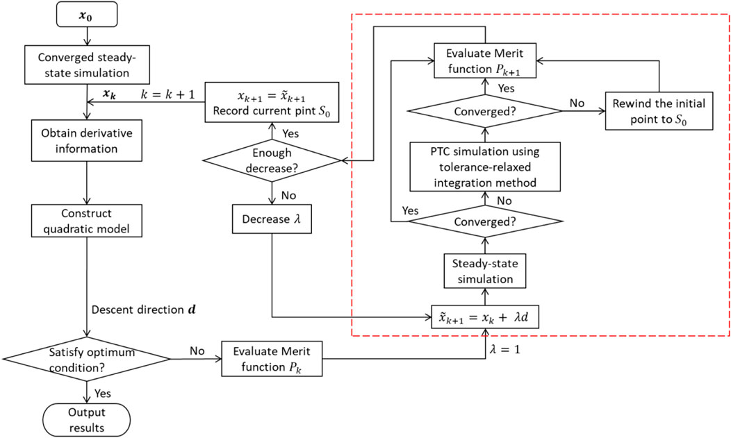
Our previous proposed hybrid feasible path optimisation algorithm (Ma et al., 2020) depicted in Figure 1 is employed to solve the NLP subproblem at each node. It is a combination of the steady-state simulation and the PTC simulation. The main idea of the hybrid algorithm is that a steady-state simulation is performed first. Only when it fails, a PTC simulation using the tolerance-relaxation integration method is then conducted. This is because the PTC simulation is more time consuming than the steady-state simulation. The initial values for the decision variables must result in a converged simulation from which the hybrid algorithm can start. Once the steady-state simulation is converged, the derivative information calculated together with the determined dependent variables through the process simulation are provided to the gradient-based optimiser in the outer lever. If the optimal conditions such as KKT (Karush-Kuhn-Tucker) conditions are satisfied, then the optimal solution is obtained, and simulation is terminated. Otherwise, the optimiser will use the provided gradient information and the values of decision variables to construct quadratic models and generate the descent direction $d$. By applying the step length $\lambda$ to the descent direction $d$, a new set of decision variables is created and returned to the process simulator to perform steady-state simulation.

FIGURE 1

FIGURE 1. Steady state and PTC simulation algorithm.

If the simulation converges, the next iteration can be started. Otherwise, a PTC simulation will be performed to generate a converged simulation. However, if the PTC simulation also fails, step length $\lambda$ will be reduced. If the PTC simulation is successful, the merit function will be evaluated based on whether a sufficient decrease is obtained. If so, next iteration can be started. Otherwise, step length shall be decreased and steps circled out in the red rectangle in Figure 1 will be repeated until enough decrease is obtained or the maximum number of line searches is met. If the acceptable step length cannot be found within maximum number of line searches, the last step will be accepted anyway. Figure 1 illustrates the hybrid steady-state and PTC simulation algorithm. The detailed steps are described below:

Step 1: When $k=0$, initial values that make steady-state process simulation converge are given to decision variables ${\mathit{x}}_0$.

Step 2: Obtain derivative information of the objective function and constraint functions with respect to decision variables ${\mathit{x}}_k$ from process simulator.

Step 3: Construct a quadratic programming (QP) problem and solve to get the descent direction $d$ and estimated Lagrange multipliers.

Step 4: If the KKT conditions are satisfied, the optimal solution is found and proceed to the final step. Otherwise go to next step.

Step 5: Evaluate the merit function $P_k$ with $x_k$ and set the step length $\lambda$ to 1.

Step 6: A group of trial decision variables ${\stackrel{\sim }{x}}_{k+1}$ are obtained by applying the step length $\lambda$ to the descent direction $d$, where ${\stackrel{\sim }{x}}_{k+1}=x_k+\lambda d$.

Step 7: Conduct steady-state simulation using ${\stackrel{\sim }{x}}_{k+1}$. If simulation fails, go to next step. Otherwise, proceed to Step 10.

Step 8: Conduct the PTC simulation using the tolerances-relaxation integration method. If converged, go to Step 10. Otherwise, go to next step.

Step 9: Set the objective function to a large value (e.g., $1\times {10}^{15}$) and rewind the values of all dependent variables in the current simulation to those in the converged simulation solution (denoted as $S_0$) from last iteration (iteration $k-1$).

Step 10: Evaluate new merit function $P_{k+1}$. If it achieves a sufficient decrease compared to $P_k$, then accept current trial decision variables as $x_{k+1}$. Record current simulation solution as $S_0$. The line search is complete and return to Step 2. If not enough decrease, reduce the step length by cutting it half and return to Step 6.

Step 11: Output results.

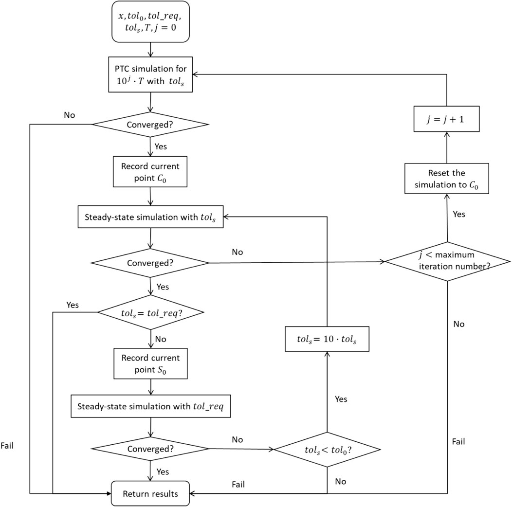
As the PTC simulation is more time-consuming than the steady-state simulation, a tolerances-relaxation integration method which is illustrated in Figure 2 is used in combination with PTC simulation to save the computational effort. When the first attempted steady-state simulation with required tolerance fails, the dynamic simulation using PTC models shall be conducted with a large integration tolerance in the beginning. A presumably long enough integration time $\mathrm{T}$ is used to ensure the solution close to the steady-state solution before the required tolerance is used. Using the solution from dynamic simulation with a large integration tolerance as initial points, a steady state simulation with the same large tolerance is then conducted. If simulation converges, a direct steady state simulation with required tolerance is performed. In most cases, the direct steady state simulation is fast and converged. However, if it fails, dynamic simulations using the gradual loosen tolerance shall be performed to find a “closer” solution to the steady state solution. In the meanwhile, as the tolerance gets smaller, the integration time is increased to ensure that the solution from dynamic simulation is close enough to the true steady state solution. The detailed steps are described below:

FIGURE 2

FIGURE 2. Tolerances relaxation integration method.

Step 1: Given values of the decision variables from last converged steady-state simulation, an integration time $T$, the largest tolerance $to{l}_0$, the required tolerance $tol\_req$ and the simulation tolerance $to{l}_s$ which has the same initial value as $to{l}_0$. The iteration indicator $j$ for integration time is initially set to zero.

Step 2: Run dynamic simulation for PTC models for pseudo time ${10}^j\cdot T$ with tolerance $to{l}_s$. If the PTC simulation fails, the whole process simulation fails and then goes to Step 8. Otherwise, go to next step.

Step 3: Record current converged point as $C_0$. Run steady-state simulation with $to{l}_s$. If converged, go to Step 6. Otherwise, go to next step.

Step 4: If $j$ reaches maximum iteration number, the process simulation fails and go to step 8. Otherwise, go to next step.

Step 5: Reset the initial points to $C_0$ and increase $j$ by 1 to increase the integration time. Return to Step 2.

Step 6: If $to{l}_s$ is equal to $tol\_req$, then the simulation completes successfully and go to Step 8. If $to{l}_s$ is larger than $tol\_req$ and smaller than $to{l}_0$, record current steady state solution as $S_0$ and run a steady-state simulation with $tol\_req$.

Step 7: If converged, the simulation completes successfully and go to Step 8. If fails, reset the process variables to points $S_0$ and magnify $to{l}_s$ by 10 times and then return to Step 2. If $to{l}_s$ is larger than $to{l}_0$, the process simulation fails and go to Step 8.

Step 8: Return results.

3.2 FPBB algorithm

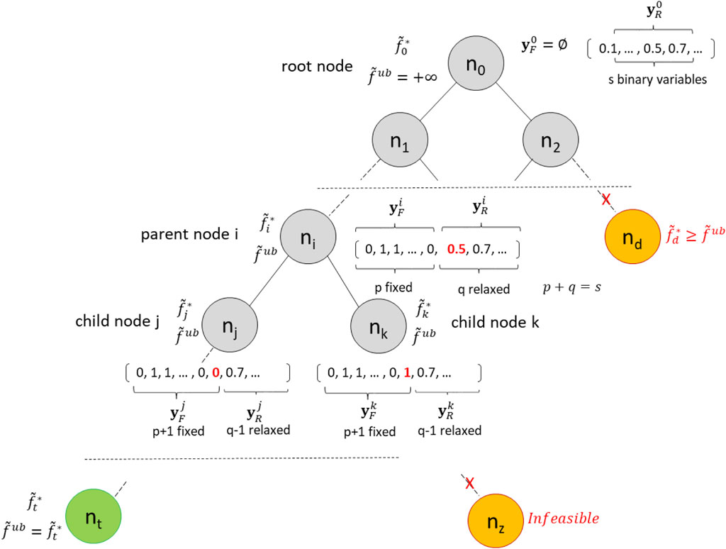
The branch and bound search tree constructed by FPBB algorithm is illustrated in Figure 3. The root node is denoted as $n_0$, at which an NLP problem is to be solved. This NLP problem is a relaxation of the problem P2 with all the binary variables relaxed to be 0–1 continuous variables. At the root node, only root node is contained in active nodes set $\zeta$. The fixed binary set ${\mathit{y}}_F^0$ is empty, while the relaxed binary set ${\mathit{y}}_R^0$ contains all the binary variables with assigned initial values that need to be determined. The upper bound ${\stackrel{\sim }{f}}^{ub}$ is set to infinite.

FIGURE 3

FIGURE 3. FPBB branch and bound search tree.

After solving the root node, the optimal results in ${\mathit{y}}_R^{0*}$ shall be examined. If all the determined values are already 0 or 1, the algorithm should be terminated with the integer solution from root node. Otherwise, two new child nodes are created. The active set $\zeta$ will be updated with two new nodes $n_1$ and $n_2$, with $n_0$ deleted from it.

The NLP subproblem to be solved at node $n_i$ is formulated as problem P7.

$\begin{array}{l}\underset{x_I,y_R^i}{\min }\stackrel{\sim }{f}\left({\mathbf{x}}_{\mathrm{I}},{\mathbf{y}}_{\mathrm{R}}^{\mathrm{i}};{\mathbf{y}}_{\mathrm{F}}^{\mathrm{i}}\right)\\ s.t.\stackrel{\sim }{\mathbf{h}}\left({\mathbf{x}}_{\mathrm{I}},{\mathbf{y}}_{\mathrm{R}}^{\mathrm{i}};{\mathbf{y}}_{\mathrm{F}}^{\mathrm{i}}\right)=0\\ \stackrel{\sim }{\mathbf{g}}\left({\mathbf{x}}_{\mathrm{I}},{\mathbf{y}}_{\mathrm{R}}^{\mathrm{i}};{\mathbf{y}}_{\mathrm{F}}^{\mathrm{i}}\right)\le 0\\ {\mathbf{x}}_{\mathrm{I}}\in R^{n-m},{\mathbf{y}}_{\mathrm{R}}^{\mathrm{i}}\in {\left(\mathrm{0,1}\right)}^q,{\mathbf{y}}_{\mathrm{F}}^{\mathrm{i}}\in {\left\{\mathrm{0,1}\right\}}^p\end{array}(\mathrm{P7})$

At each node $n_i$, our previous introduced hybrid steady-state and time-relaxation-based optimisation algorithm is employed to solve the NLP subproblem. After solving the NLP subproblem at node $n_i$, the pruning rules shall be applied. If there is no feasible solution at node $n_i$, then this node is pruned. If an optimal solution ${\stackrel{\sim }{f}}_i^{*}$ exists, it shall be compared with the upper bound ${\stackrel{\sim }{f}}^{ub}$ which is either infinite (no optimal integer solution so far) or current best integer solution. If ${\stackrel{\sim }{f}}_i^{*}$ is larger than ${\stackrel{\sim }{f}}^{ub}$, the node will also be pruned. Otherwise, ${\mathit{y}}_R^{i*}$ shall be checked. If all the components in ${\mathit{y}}_R^{i*}$ are binaries, it means solution at node $n_i$ is an optimal integer solution. Then ${\stackrel{\sim }{f}}^{ub}$ will be updated to ${\stackrel{\sim }{f}}_i^{*}$. If some components in ${\mathit{y}}_R^{i*}$ are still fractions, node $n_i$ will be treated as a parent node and further branched where one relaxed binary variable in ${\mathit{y}}_R^{i*}$ with value close to 0.5 is selected and forced to 0 or 1. Hereby two child nodes $n_j$ and $n_k$ will be created. Obviously, only one binary variable in nodes $n_j$ and $n_k$ is different from their parent node $n_i$. Hence the optimal solution from parent node is used to initialise the NLP subproblems in its child nodes.

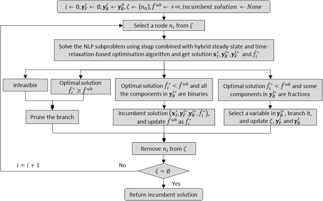
The depth-first search strategy is used to select which of the candidate subproblems (i.e., active nodes) in $\zeta$ to solve. The chosen node will be explored again using FPBB algorithm in Figure 4.

FIGURE 4

FIGURE 4. FPBB algorithm.

3.3 Implementation

In this work, the process flowsheet models are written in the equation-oriented modelling environment - Aspen Custom Modeler (ACM). The convenience of using process simulators is that it possesses unit operation models, submodels to calculate physical properties, and flow-sheeting capabilities (Franke, 2017). The solution is more practical since it can be applied to nonideal systems without making simplifying assumptions such as the ideality on liquid and gas phase. Compared to the sequential modular (SM) environment such as Aspen Plus, the advantage of conducting process simulations in the EO environments is that Jacobian and Hessian matrices can be calculated via automatic differentiation which enables the simultaneous solution of large-scale nonlinear equations (Dowling and Biegler, 2015). The NLP subproblems are decomposed into two layers. The outer layer is a small optimisation problem, while the inner layer is a process simulation problem. For simulations in the equation oriented (EO) environment, the most widely used method for solving these problems, however, is Newton’s method. It works best only when the starting point is near to an optimal point. To resolve such problems, we apply the steady-state and time-relaxation based algorithm together with PTC models to each NLP subproblem. A larger basin of initial conditions is achieved, and convergence can be guaranteed.

The FPBB algorithm is implemented in Python. Open-source optimiser slsqp (Kraft, 1988) is the selected NLP solver for the outer layer optimisation. Information such as derivatives and iterative values of variables transferred between Python and ACM is via ACM automation interface.

4 Computational studies

To illustrate the capability and superiority of the proposed FPBB algorithm, three process intensification problems (i.e., DWC) and two process synthesis problems (i.e., distillation sequences synthesis) are solved. The first two examples are taken from Montonati et al. (2022) and involve the separation of ternary hydrocarbon mixtures. Example 3 requires the separation of a four-component mixture in a Kaibel column. Example 4 involves optimisation of a distillation sequence synthesis for the separation of a mixture of benzene, toluene, and o-xylene. Example 5 is the separation of a four-component mixture of methanol, ethanol, 1-propanol and 1-butanol. All examples are modelled with rigorous models. Bypass efficiency $\left({\epsilon }^n\right)$ (Dowling and Biegler, 2014) is adopted to model the number of trays and treated as binary variables in our study which gives the flexibility of optimising the feed stage location, side draw location and the number of stages in a distillation column. The complete mathematical model is provided in Supplementary Material.

The objective function of these five case studies is stated as below:

$\min TAC=f\left(N_{true},D,A_R,A_c\right)+C_s\cdot Q_R+C_w\cdot Q_C$

where $N_{true}$ stands for the actual number of stages, $D$ is the diameter of the column, and $A_R$ and $A_c$ are the reboiler area and condenser area respectively, $C_s$ and $C_w$ are the steam and cooling water costs, $Q_R$ and $Q_C$ are the reboiler and condenser duties, the function $f\left(\cdot \right)$ represents annualised capital cost.

In each example, the optimisation tolerance is set as $1\times {10}^{-5}$. The largest simulation tolerance used in the tolerances-relaxation method is $1\times {10}^{-3}$, while the required simulation is $1\times {10}^{-9}$. All examples are solved on a laptop with a 1.9 GHz Intel Core i7 processor and 8 GB of RAM running Windows 10 64-bit operating system.

4.1 Example 1: Separation of n-pentane, n-hexane and n-heptane

In this example, a DWC is used for the separation of a ternary mixture consisting of n-pentane, n-hexane and n-heptane. DWC is a practical implementation which integrates two columns into a single shell by the addition of a wall that physically separates the feed side from the side product draw off section. It has been proven that up to 30% energy savings can be achieved together with space and capital cost reduction (Babi et al., 2016). Optimal design of DWC is not straightforward since it possesses a complex structure with additional design parameters to be considered, such as vapour and liquid split ratio and side draw flowrate.

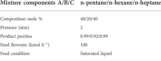
Table 1 provides information on feed conditions, product specifications, and column operating pressure, which is fixed in this example. The Peng-Robinson equation of state was used for the vapor-liquid equilibrium calculation.

TABLE 1

TABLE 1. Feed conditions for Example 1.

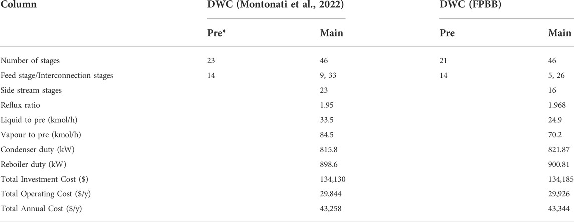
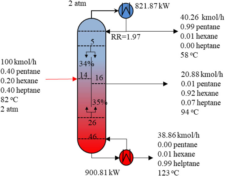
The decision variables include bypass efficiency, reflux ratio, reboiler vaporization fraction, side draw fraction, liquid and vapour split ratio. We use the proposed FPBB algorithm to solve this example. The optimisation problem involves 180 binary variables, 21,167 continuous variables and 18,965 constraints. We generate a locally optimal solution of 43,344 $ yr⁻¹ within 2,712 CPU s. The optimal results are provided in Table 2. From Table 2, it can be observed that in the optimal design, there are 46 trays in the main column and 23 trays in the prefractionator column. The optimal design is illustrated in Figure 5.

TABLE 2

TABLE 2. Optimal design for Example 1.

FIGURE 5

FIGURE 5. Optimal design and operating conditions of DWC column for Example 1.

The conventional sequence of separation has a low thermodynamic efficiency due to the remixing effect (the remixing of internal streams with different compositions that occurs at the feed point and along column). This is eliminated or reduced by the design of DWC (Dejanovic et al., 2010). As shown in Figure 6, the side draw is located on the 16th tray where the concentration of middle boiling component n-hexane is close to its peak concentration as shown in Figure 6. This significantly reduces the re-mixing effects in two columns in series arrangements, which is one of the primary reasons why DWC uses much less energy than conventional configurations. Another gain in this respect is that as the prefractionator distributes intermediate component between top and bottom, there is a greater freedom in matching the feed composition with a tray in the column to further reduce mixing losses at the feed tray. This also can be substantiated in our results. The feed stream contains 20% n-hexane which matches with the composition of 21.37% n-hexane in the feed tray.

FIGURE 6

FIGURE 6. Composition profiles of Toluene in the DWC for Example 1.

The computational performance of the proposed FPBB algorithm is presented in Table 3. From Table 3, it shows 9 nodes are created and investigated during B&B, and all the 9 NLP subproblems have been solved successfully. Interestingly, during B&B, three feasible integer solutions are found. Two nodes are pruned due to the optimal solution is larger than the upper bound. In the final optimal integer solution, all the bypass efficiencies are at 0 or 1.

TABLE 3

TABLE 3. Computational performance for Example 1.

We also compare the optimal design with that from literature (Montonati et al., 2022), which is generated using the specialised or heuristic procedure. The comparative results are also provided in Table 2. From Table 2, it can be observed that the configuration obtained by using FPBB is very similar to the configuration in the literature (Montonati et al., 2022). The method used in the literature (Montonati et al., 2022) is a special procedure, which requires short-cut models to determine the initial design parameters of DWC, followed by equilibrium-staged simulation, molecular tracking application and finally using many simulations to investigate the effects of varying parameters in the flowsheet to find an optimal design. The design procedure is tailored without generality and computationally intensive for design of DWC. The total computational time is not reported. By applying our algorithm to the same case, the total computational time is 2,712 CPU s.

4.2 Example 2: Separation of n-butane, i-pentane, n-pentane

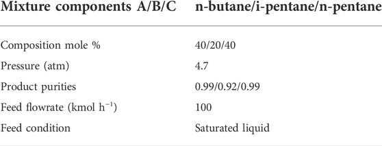
Similar to Example 1, Example 2 consists of a mixture of n-butane, i-pentane and n-pentane to be separated in a DWC. As the boiling points of i-pentane and n-pentane are quite close, the separation is more difficult than the mixture in Example 1. This is reflected on the number of stages in the DWC column. Table 4 provides information on the feed properties. Operating column pressure is also fixed in this example.

TABLE 4

TABLE 4. Feed conditions for Example 2.

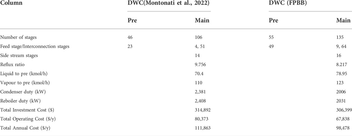
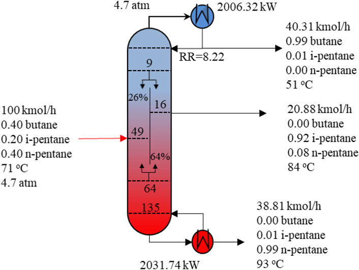
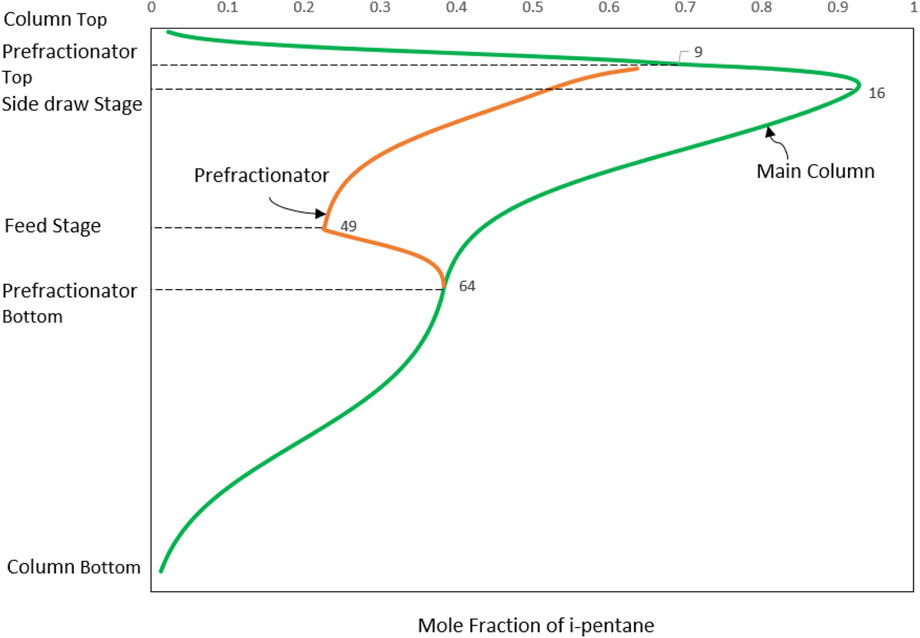
The optimisation problem involves 350 binary variables, 35,955 continuous variables and 36,305 equations. Compared to Example 1, the size of Example 2 problem is much larger. This is reflected on the prolonged CPU time and nodes generated and evaluated. The resulting configuration from the FPBB algorithm is compared with the corresponding configuration using molecular tracking from the literature (Montonati et al., 2022). The results are presented in Table 5. These two configurations are rather different. From Table 5, we can see that the total number of trays obtained from the FPBB algorithm is 135, which is 28 more than 106 in the literature (Montonati et al., 2022). The larger number of stages results in a smaller reflux ratio and less energy consumption in both condenser and reboiler. The heat duty in the reboiler is 15.7% less than the heat duty of the reboiler in the literature. The operating cost is reduced by 15.6%. Though our DWC column possesses more stages, the capital cost for condenser and reboiler is reduced due to less area required. As a result, a locally optimal solution 98, 478 $ yr⁻¹ is found with 12% TAC reduction compared to the TAC from the literature. Figure 7 illustrates the optimal design of DWC. The composition profiles of i-pentane in the column is provided in Figure 8. From Figure 8, it can be seen that the intermediate component i-pentane is drawn on the 16th tray near to its maximum composition, which avoids the effect of re-mixing. The composition of i-pentane on the fee tray is 22.74% which is close to its composition 20% in the feed stream.

TABLE 5

TABLE 5. Optimal design for Example 2.

FIGURE 7

FIGURE 7. Optimal design and operating conditions of DWC column for Example 2.

FIGURE 8

FIGURE 8. Composition profiles of i-pentane in the DWC for Example 2.

The computational performance is presented in Table 6. 47 nodes are evaluated 24 nodes are pruned due to the optimal solution larger than the upper bound. 4 integer solutions are found.

TABLE 6

TABLE 6. Computational performance for Example 2.

4.3 Example 3: Separation of n-butane, n-pentane, n-hexane and n-heptane

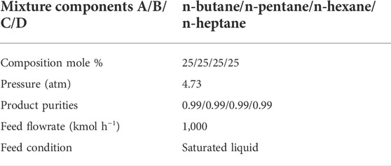
This example is taken from Errico et al. (2009). The authors studied the possible energy saving using a DWC together with a simple column for the separation of a four-component mixture. In our study, the four-component mixture is separated using one DWC, commonly referred to in the literature as a Kaibel column (Kaibel, 1987). The configuration of a Kaibel column is similar to the above two DWC configurations. The only difference is that two side draws exist on the right side of the divided wall. Feed conditions, product specifications, and the other operative conditions considered in this example are summarized in Table 7. In the literature (Errico et al., 2009), the pressure of feed streams is 1 atm, which is not practical since the column pressure is 4.73 atm. In our work, the pressure of feed is changed to 4.73 atm to make it consistent with column pressure. However, in order to make results comparative, computational results for the case with the pressure of 1 atm are also presented in Table 8.

TABLE 7

TABLE 7. Feed conditions for Example 3.

TABLE 8

TABLE 8. Optimal design for Example 3.

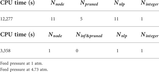
The optimisation problem involves 240 binary variables, 28,121continuous variables and 28,361 constraints. Table 9 provides the computational performance. For the case with feed pressure at 1 atm, the optimisation consumes 12, 277 CPU s. Total 11 nodes are evaluated. 4 nodes are pruned due to maximum iteration number reached. 1 node is pruned due to the lower bound larger than the upper bound. Only 1 integer solution is found. For the case with feed pressure at 4.73 atm, the optimal integer solution is found at root node within 3,358 CPU s.

TABLE 9

TABLE 9. Computational performance for Example 3

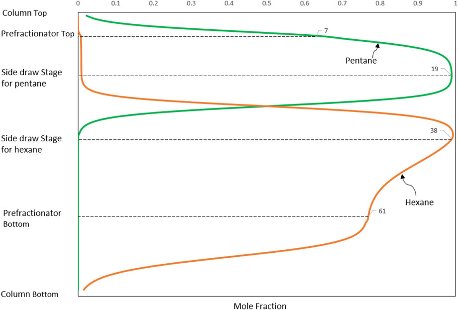
The detailed results with comparison to the results in the literature (Errico et al., 2009) are also provided in Table 8. The column configuration is illustrated in Figure 9. From Table 8, it can be seen that the reboiler duty is 14262.86 kW for the case with feed pressure at 1 atm, which can be reduced by 12.5% compared to that (16297.27 kW) from the literature (Errico et al., 2009). When the feed pressure increases to 4.73 atm, the reboiler duty decreases to 12025.42 kW, which is further reduced by 26.2% compared to that (16297.27) at 1 atm. As indicated by Errico et al. (2009), the capital cost evaluation of DWC is not defined. Therefore, comparison can only be made in terms of energy savings. The significant reduction of reboiler duty is due to the avoidance of remixing effect which can be substantiated by the composition profiles in the Kaibel column in Figure 10. From Figure 10, it can be observed that both n-pentane and n-hexane are drawn near to their peak compositions in the column to avoid the effect of remixing.

FIGURE 9

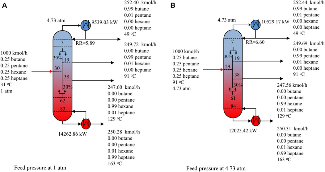
FIGURE 9. Optimal design and operating conditions of Kaibel column for Example 3. (A) Feed pressure at 1 atm. (B) Feed pressure at 4.73 atm.

FIGURE 10

FIGURE 10. Composition profiles of Pentane and Hexane in the Kaibel column for Example 3

4.4 Example 4: Separation of benzene, toluene and o-xylene

The superstructure for synthesis of distillation sequences is constructed using the state-equipment network (SEN). In comparison to the state-task network (STN), SEN representation requires fewer equipment, leading to a smaller combinatorial problem for the selection of equipment. As a result, a smaller model can be obtained (Yeomans and Grossmann, 1999). The superstructure (Yeomans and Grossmann, 2000) is presented in Supplementary Figure S1. The decision variables for process sequence synthesis include bypass efficiency, reflux ratio, reboiler vaporization ratio and split fractions.

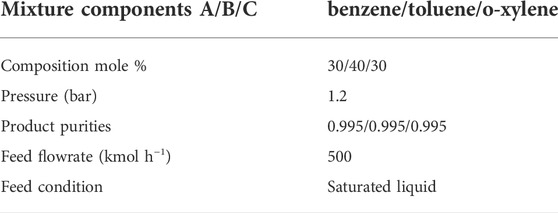
For this example, we conduct a distillation sequence synthesis for a feed mixture of benzene, toluene and o-xylene. Product specifications and the other operating conditions considered are summarized in Table 10. We also use the proposed FPBB algorithm to solve. The computational results are provided in Table 11. This optimisation problem involves 122 binary variables, 14,552 continuous variables and 13,052 constraints. From Table 11, it can be observed that CPU time is 1,723 s with 3 nodes evaluated. 1 node is pruned due to the optimal value of objective function larger than the upper bound.

TABLE 10

TABLE 10. Feed conditions for Example 4.

TABLE 11

TABLE 11. Computational performance for Example 4.

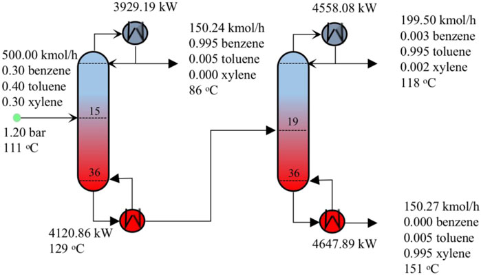
The optimal distillation sequence with the minimum TAC of 2,325,271 $ yr⁻¹ is illustrated in Figure 11, which is direct distillation sequence for this example. If column sequencing heuristics are applied to select the separation sequence, the rules in the book by Smith (2016) should be obeyed. The first rule is to perform easy separation where the adjacent components have the highest relative volatility. The relative volatilities ${\alpha }_{B,X}/{\alpha }_{T,X}/{\alpha }_{X,X}$ are approximately 7.1/2.2/1. As the relative volatility of benzene and toluene is larger than that of toluene and o-xylene, separation of benzene should be performed first. The second rule is to remove the component comprising a large fraction of the feed first. Since the feed stream contains benzene and o-xylene equality. This rule also cannot be used to determine the sequence. The third rule is to remove the lightest component alone by one in column overheads. In other words, direct sequence is favoured. By using the heuristic rule approach, direct separation sequence is selected which is consistent with our optimisation result.

FIGURE 11

FIGURE 11. Optimal distillation sequence with operating conditions for Example 4.

4.5 Example 5: Separation of methanol, ethanol, 1-propanol and 1-butanol

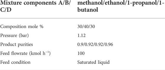
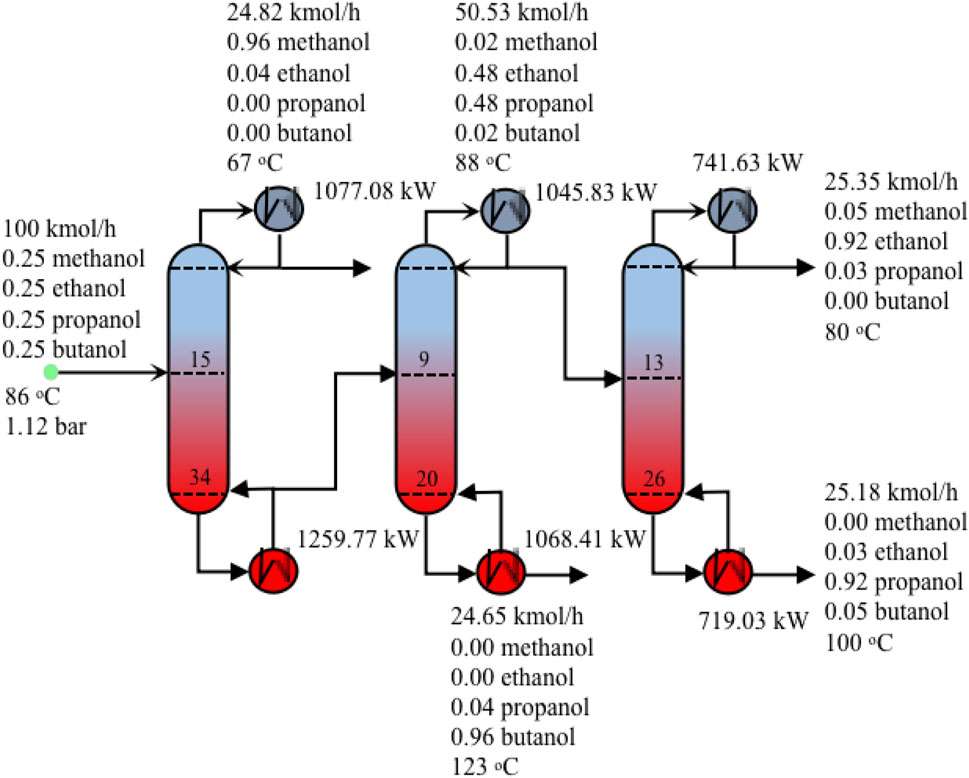
This example is to separate a four-component mixture consisting of methanol, ethanol, 1-propano and 1-butanol. The feed conditions are summarised in Table 12. The SEN superstructure (Yeomans and Grossmann, 2000) for separation of methanol, ethanol, 1-propanol and 1-butanol is provided in Supplementary Figure S1. The logic constraints that enforce the consistency of tasks in the columns are provided in the Supplementary Material. The operating pressure is assumed to be constant throughout these three columns, with a value of 112 kPa. This problem involves 190 binary variables, 24,881 continuous variables, 22,058 equality constraints and 41 inequality constraints. Figure 12 shows the optimal separation sequence with operating conditions. Methanol is separated first because the heuristics approach favours the first separation of the lightest component. Then it is followed by the separation of heaviest component 1-butanol. The separation of ethanol and 1-propanol comes at last. Table 13 presents the computational results. As seen from Table 13, CPU time is 2,470 s with 3 nodes evaluated. 1 node is pruned due to infeasibility.

TABLE 12

TABLE 12. Feed conditions for Example 5.

FIGURE 12

FIGURE 12. Optimal distillation sequence with operating conditions for Example 5.

TABLE 13

TABLE 13. Computational performance for Example 5.

5 Conclusion

In this work, a novel feasible-path based branch and bound algorithm was proposed, where the branch and bound method was used to systematically fix part of the binary variables and generate relaxed NLP subproblems, while the hybrid steady state and time relaxation-based feasible path algorithm was employed to solve the derived NLP subproblems. In the generated B&B tree, the solution from the parent node is provided as a warm start for the NLP subproblems at the child nodes, which increases the computational efficiency. Five example problems were solved to evaluate the robustness and performance of the proposed algorithm. They demonstrated that the proposed algorithm was able to find a locally optimum with very good convergence performance. The first three problems showed that it was capable of solving the optimization of DWC for separation of a ternary/quaternary mixture within an acceptable time. Though FPBB achieved similar DWC configuration and TAC for Example 1 compared to the results in the literature, the CPU time was 2,712 s and FPBB did not require specialised procedure for the design of DWC. Moreover, for Examples 2 and 3, energy savings could be up to 15% using FPBB. The last two examples illustrated that it was able to be used for process synthesis problems. The optimal solution for distillation sequence synthesis problems was found in 1,723 CPU s for a ternary mixture and 2,470 CPU s for a quaternary mixture. As the models are written in an EO environment ACM for inner level simulation and connected to Python for outer level optimization, data transfer time between the software consumes at least one-third of CPU time. It should be noted that the proposed algorithm cannot guarantee a global optimum since the nonconvex NLP subproblems are solved to local optimality for efficiency.

In the future, a comprehensive evaluation of the proposed FPBB algorithm will be conducted by solving a variety of nonconvex MINLP problems. Detailed comparison of the proposed FPBB algorithm with some existing MINLP algorithms will also carried out. The advantages and disadvantages of the proposed algorithm will be clearly identified. In addition, this novel MINLP algorithm can be further applied to other process intensification cases such as reactive distillation and membrane reactor and process synthesis problems such as superstructure flowsheets coupled with reactors. Efforts should also be made on finding the global optimum within an acceptable computational time.

Data availability statement

The original contributions presented in the study are included in the article/Supplementary Material, further inquiries can be directed to the corresponding author.

Author contributions

CL: Conceptualisation (equal); data curation (equal); formal analysis (lead); investigation (lead); methodology (equal); software (lead); validation (lead); writing–original draft (lead); writing–review and editing (equal). YM: Conceptualisation (equal); data curation (equal); investigation (equal); methodology (equal); software (equal). DZ: Methodology (equal); resources (equal); supervision (lead); writing–review and editing (equal). JL: Conceptualisation (equal); data curation (equal); funding acquisition (lead); methodology (equal); resources (equal); supervision (lead); writing–review and editing (equal).

Funding

PhD scholarship from Department of Chemical Engineering, The University of Manchester. China Scholarship Council–The University of Manchester Joint Scholarship (201809120005).

Acknowledgments

CL would like to appreciate financial support from The University of Manchester. YM acknowledges financial support from China Scholarship Council–The University of Manchester Joint Scholarship (201809120005).

Conflict of interest

The authors declare that the research was conducted in the absence of any commercial or financial relationships that could be construed as a potential conflict of interest.

Publisher’s note

All claims expressed in this article are solely those of the authors and do not necessarily represent those of their affiliated organizations, or those of the publisher, the editors and the reviewers. Any product that may be evaluated in this article, or claim that may be made by its manufacturer, is not guaranteed or endorsed by the publisher.

Supplementary material

The Supplementary Material for this article can be found online at: https://www.frontiersin.org/articles/10.3389/fceng.2022.983162/full#supplementary-material

Abbreviations

ACM, Aspen Custom Modeler; BB, Branch and Bound; FPBB, Feasible Path-based Branch and Bound Algorithm; MINLP, Mixed Integer Nonlinear Programming; PTC, Pseudo-Transient Continuation; NLP, Nonlinear Programming; MILP, Mixed-integer Linear Programming; ECP, Extended Cutting Plane; GBD, Generalised Bender Decomposition; GDP, Disjunction Programmin; OA, Outer Approximation; SBB, Standard Nonlinear Branch and Bound; ODE, Ordinary Differential Equation; DAE, Differential Algebraic Equation; TAC, Total Annualized Cost; DWC, Dividing-Wall Column; MESH, Mass, Equilibrium, Summation and Heat; EO, Equation-oriented.

References

Amjadian, A., and Gharaei, A. (2021). An integrated reliable five-level closed-loop supply chain with multi-stage products under quality control and green policies: Generalised outer approximation with exact penalty. Int. J. Syst. Sci. Operations Logist.,9 429–449. doi:10.1080/23302674.2021.1919336

CrossRef Full Text | Google Scholar

Androulakis, I. P., Maranas, C. D., and Floudas, C. A. (1995). αBB: A global optimization method for general constrained nonconvex problems. J. Glob. Optim. 7 (4), 337–363. doi:10.1007/bf01099647

CrossRef Full Text | Google Scholar

Battisti, R., Claumann, C. A., Marangoni, C., and Machado, R. A. F. (2019). Optimization of pressure-swing distillation for anhydrous ethanol purification by the simulated annealing algorithm. Braz. J. Chem. Eng. 36 (1), 453–469. doi:10.1590/0104-6632.20190361s20180133

CrossRef Full Text | Google Scholar

Burer, S., and Letchford, A. N. (2012). Non-convex mixed-integer nonlinear programming: A survey. Surv. operations Res. Manag. Sci. 17 (2), 97–106. doi:10.1016/j.sorms.2012.08.001

CrossRef Full Text | Google Scholar

Burre, J., Bongartz, D., and Mitsos, A. (2022). Comparison of MINLP formulations for global superstructure optimization. Optimization and engineering. New York City: Springer. doi:10.1007/s11081-021-09707-y

CrossRef Full Text | Google Scholar

Dejanovic, I., Matijasevic, L., and Olujic, Z. (2010). Dividing wall column—a breakthrough towards sustainable distilling. Chem. Eng. Process. Process Intensif. 49 (6), 559–580. doi:10.1016/j.cep.2010.04.001

CrossRef Full Text | Google Scholar

Dowling, A. W., and Biegler, L. T. (2015). A framework for efficient large scale equation-oriented flowsheet optimization. Comput. Chem. Eng. 72, 3–20. doi:10.1016/j.compchemeng.2014.05.013

CrossRef Full Text | Google Scholar

Dowling, A. W., and Biegler, L. T. (2014). “Rigorous optimization-based synthesis of distillation Cascades without integer variables,” in Computer aided chemical engineering, 55–60.

CrossRef Full Text | Google Scholar

Errico, M., Tola, G., Rong, B. G., Demurtas, D., and Turunen, I. (2009). Energy saving and capital cost evaluation in distillation column sequences with a divided wall column. Chem. Eng. Res. Des. 87 (12), 1649–1657. doi:10.1016/j.cherd.2009.05.006

CrossRef Full Text | Google Scholar

Farkas, T., Czuczai, B., Rev, E., and Lelkes, Z. (2008). New MINLP model and modified outer approximation algorithm for distillation column synthesis. Ind. Eng. Chem. Res. 47 (9), 3088–3103. doi:10.1021/ie0711426

CrossRef Full Text | Google Scholar

Flores-Tlacuahuac, A., and Biegler, L. T. (2007). Simultaneous mixed-integer dynamic optimization for integrated design and control. Comput. Chem. Eng. 31 (5), 588–600. doi:10.1016/j.compchemeng.2006.08.010

CrossRef Full Text | Google Scholar

Floudas, C. A. (2009). “Mixed integer nonlinear programming,” in Encyclopedia of optimization. Editors C. A. FLOUDAS, and P. M. PARDALOS (Boston MA: Springer US).

Google Scholar

Franke, M. B. (2017). Design of dividing wall columns by mixed integer nonlinear programming optimization. Chem. Ing. Tech. 89 (5), 582–597. doi:10.1002/cite.201700005

CrossRef Full Text | Google Scholar

Geoffrion, A. M. (1972). Generalized benders decomposition. J. Optim. Theory Appl. 10, 237–260. doi:10.1007/bf00934810

CrossRef Full Text | Google Scholar

Grossmann, I. E. (2012). Advances in mathematical programming models for enterprise-wide optimization. Comput. Chem. Eng. 47, 2–18. doi:10.1016/j.compchemeng.2012.06.038

CrossRef Full Text | Google Scholar

Gupta, O. K., and Ravindran, A. (1985). Branch and bound experiments in convex nonlinear integer programming. Manag. Sci. 31 (12), 1533–1546. doi:10.1287/mnsc.31.12.1533

CrossRef Full Text | Google Scholar

Jackson, J. R., and Grossmann, I. E. (2001). A disjunctive programming approach for the optimal design of reactive distillation columns. Comput. Chem. Eng. 25 (11), 1661–1673. doi:10.1016/s0098-1354(01)00730-x

CrossRef Full Text | Google Scholar

Kronqvist, J., and Lundell, A. (2019). Convex minlp–an efficient tool for design and optimization tasks? Computer aided chemical engineering. Nertherland: Elsevier.

Google Scholar

Kaibel, G. (1987). Distillation columns with vertical partitions. Chem. Eng. Technol. 10 (1), 92–98. doi:10.1002/ceat.270100112

CrossRef Full Text | Google Scholar

Kilinç, M. R., and Sahinidis, N. V. (2017). Chapter 21: State of the art in mixed-integer nonlinear optimization. Advances and trends in optimization with engineering applications. Pennsylvania:: Siam.

Google Scholar

Kraft, D. (1988). A software package for sequential quadratic programming, wiss. Germany: Berichtswesen d. DFVLR.

Google Scholar

Kronqvist, J., Bernal, D. E., Lundell, A., and Grossmann, I. E. (2018). A review and comparison of solvers for convex MINLP. Optim. Eng. 20 (2), 397–455. doi:10.1007/s11081-018-9411-8

CrossRef Full Text | Google Scholar

Kronqvist, J., Lundell, A., and Westerlund, T. (2015). The extended supporting hyperplane algorithm for convex mixed-integer nonlinear programming. J. Glob. Optim. 64 (2), 249–272. doi:10.1007/s10898-015-0322-3

CrossRef Full Text | Google Scholar

Lee, S., and Grossmann, I. E. (2000). New algorithms for nonlinear generalized disjunctive programming. Comput. Chem. Eng. 24 (9), 2125–2141. doi:10.1016/s0098-1354(00)00581-0

CrossRef Full Text | Google Scholar

Liñán, D. A., Bernal, D. E., Gomez, J. M., and Ricardez-Sandoval, L. A. (2021). Optimal synthesis and design of catalytic distillation columns: A rate-based modeling approach. Chem. Eng. Sci. 231, 116294. doi:10.1016/j.ces.2020.116294

CrossRef Full Text | Google Scholar

Lutze, P., Gani, R., and Woodley, J. M. (2010). Process intensification: A perspective on process synthesis. Chem. Eng. Process. Process Intensif. 49 (6), 547–558. doi:10.1016/j.cep.2010.05.002

CrossRef Full Text | Google Scholar

Ma, Y., and Li, J. (2022). Homotopy continuation enhanced branch and bound algorithms for strongly nonconvex mixed‐integer nonlinear optimization. AIChE J. 68 (6). doi:10.1002/aic.17629

CrossRef Full Text | Google Scholar

Ma, Y., Luo, Y., and Yuan, X. (2017). Simultaneous optimization of complex distillation systems with a new pseudo-transient continuation model. Ind. Eng. Chem. Res. 56 (21), 6266–6274. doi:10.1021/acs.iecr.7b00380

CrossRef Full Text | Google Scholar

Ma, Y., McLaughlan, M., Zhang, N., and Li, J. (2020). Novel feasible path optimisation algorithms using steady-state and/or pseudo-transient simulations. Comput. Chem. Eng. 143, 107058. doi:10.1016/j.compchemeng.2020.107058

CrossRef Full Text | Google Scholar

McCormick, G. P. (1976). Computability of global solutions to factorable nonconvex programs: Part I - convex underestimating problems. Math. Program. 10 (1), 147–175. doi:10.1007/bf01580665

CrossRef Full Text | Google Scholar

Montonati, G., Nazemzadeh, N., Abildskov, J., and Mansouri, S. S. (2022). Divided wall distillation column design using molecular tracking. AIChE J. 68 (2). doi:10.1002/aic.17504

CrossRef Full Text | Google Scholar

Morrison, D. R., Jacobson, S. H., Sauppe, J. J., and Sewell, E. C. (2016). Branch-and-bound algorithms: A survey of recent advances in searching, branching, and pruning. Discrete Optim. 19, 79–102. doi:10.1016/j.disopt.2016.01.005

CrossRef Full Text | Google Scholar

Munawar, A., Wahib, M., Munetomo, M., and Akama, K. (2011). “Advanced genetic algorithm to solve MINLP problems over GPU,” in ProceedingIEEE Congress of Evolutionary Computation (CEC), New Orleans LA USA, 05-08 June 2011 (IEEE), 318–325. doi:10.1109/CEC.2011.5949635

CrossRef Full Text | Google Scholar

Pattison, R. C., and Baldea, M. (2014). Equation-oriented flowsheet simulation and optimization using pseudo-transient models. AIChE J. 60 (12), 4104–4123. doi:10.1002/aic.14567

CrossRef Full Text | Google Scholar

Raman, R., and Grossmann, I. (1994). Modelling and computational techniques for logic based integer programming. Comput. Chem. Eng. 18 (7), 563–578. doi:10.1016/0098-1354(93)e0010-7

CrossRef Full Text | Google Scholar

Ryoo, H., and Sahinidis, N. (1996). A branch-and-reduce approach to global optimization. J. Glob. Optim. 8 (2), 107–138. doi:10.1007/bf00138689

CrossRef Full Text | Google Scholar

Smith, R. (2016). Chemical process design and integration. Second edition. Chichester, West Sussex, United Kingdom: John Wiley & Sons.

Google Scholar

Trespalacios, F., and Grossmann, I. E. (2014). Review of mixed-integer nonlinear and generalized disjunctive programming methods. Chem. Ing. Tech. 86 (7), 991–1012. doi:10.1002/cite.201400037

CrossRef Full Text | Google Scholar

Tumbalam Gooty, R., Agrawal, R., and Tawarmalani, M. (2019). An MINLP formulation for the optimization of multicomponent distillation configurations. Comput. Chem. Eng. 125, 13–30. doi:10.1016/j.compchemeng.2019.02.013

CrossRef Full Text | Google Scholar

Türkay, M., and Grossmann, I. E. (1996). Logic-based MINLP algorithms for the optimal synthesis of process networks. Comput. Chem. Eng. 20 (8), 959–978. doi:10.1016/0098-1354(95)00219-7

CrossRef Full Text | Google Scholar

Viswanathan, J., and Grossmann, I. (1990). A combined penalty function and outer-approximation method for MINLP optimization. Comput. Chem. Eng. 14 (7), 769–782. doi:10.1016/0098-1354(90)87085-4

CrossRef Full Text | Google Scholar

Westerlund, T., and Pettersson, F. (1995). An extended cutting plane method for solving convex MINLP problems. Comput. Chem. Eng. 19, 131–136. doi:10.1016/0098-1354(95)00164-w

CrossRef Full Text | Google Scholar

Yee, T., and Grossmann, I. (1990). Simultaneous optimization models for heat integration—II. Heat exchanger network synthesis. Comput. Chem. Eng. 14 (10), 1165–1184. doi:10.1016/0098-1354(90)85010-8

CrossRef Full Text | Google Scholar

Yeomans, H., and Grossmann, I. E. (1999). A systematic modeling framework of superstructure optimization in process synthesis. Comput. Chem. Eng. 23 (6), 709–731. doi:10.1016/s0098-1354(99)00003-4

CrossRef Full Text | Google Scholar

Yeomans, H., and Grossmann, I. E. (2000). Disjunctive programming models for the optimal design of distillation columns and separation sequences. Ind. Eng. Chem. Res. 39 (6), 1637–1648. doi:10.1021/ie9906520

CrossRef Full Text | Google Scholar