Optimization of multi-mode classification for process monitoring

Process monitoring seeks to identify anomalous plant operating states so that operators can take the appropriate actions for recovery. Instrumental to process monitoring is the labeling of known operating states in historical data, so that departures from these states can be identified. This task can be challenging and time consuming as plant data is typically high dimensional and extensive. Moreover, automation of this procedure is not trivial since ground truth labels are often unavailable. In this contribution, this problem is approached as a multi-mode classification one, and an automatic framework for labeling using unsupervised Machine Learning (ML) methods is presented. The implementation was tested using data from the Tennessee Eastman Process and an industrial pyrolysis process. A total of 9 ML ensembles were included. Hyperparameters were optimized using a multi-objective evolutionary optimization algorithm. Unsupervised clustering metrics (silhouette score, Davies-Bouldin index, and Calinski-Harabasz Index) were investigated as candidates for objective functions in the optimization implementation. Results show that ensembles and hyperparameter selection can be aided by multi-objective optimization. It was found that Silhouette score and Davies-Bouldin index are strong predictions of the ensemble’s performance and can then be used to obtain good initial results for subsequent fault detection and fault diagnosis procedures.

1 Introduction

For the successful operation of any process, it is important to detect process upsets, equipment malfunctions, or other special events as early as possible, and then to find and remove the factors causing those events. As industrial processes become much more complex, thousands of process measurements need to be collected by the equipment using sensors, and analyzed to recognize equipment defects before failure, reduce costs associated with failure, maintenance costs, and improve productivity. Process Monitoring aims to ease the work of plant operators by translating high volumes of data (i.e., information from the many sensors in the plant) into readily understandable information.

As proposed by Chiang et al. (2000) process monitoring involves fault detection, fault identification, fault diagnosis and process recovery. The first step, fault detection, requires the definition of a known operating state from which the process is said to deviate. Here, we explore the issue of identifying such a known operating state from historical plant data, extended to allow for multiple known operating states. Therefore, the problem becomes a multi-mode classification one, which can in turn, at a later stage, be used for fault detection. If one or more of the known operating states are labeled as known faults, that is, faults that have been previously observed in the plant, the multi-mode classification problem can also be helpful for fault identification.

In order to identify known operating states (be it known faults or known normal operating conditions), one requires extensive process familiarity to organize the historical data into groups for each known operating state. This process, hereafter referred to as labeling, can be aided by automatic clustering techniques borrowed from the computer science literature. Clustering can be used to find intrinsic divisions within a historical dataset, often relating to separate running states within the process. Once the clustering has separated the historical data, incoming observations can be passed through a classifier to assign them to their best-matching known process state.

Clustering alone is often insufficient to adequately handle real plant data, as noise, high dimensionality, missing data, and other issues are present. Hence, clustering is typically performed within a pipeline of Data mining and knowledge discovery (DMKD). DMKD is employed to extract useful information from process data, using statistical methods and machine learning algorithms (Zhu et al., 2018; Zhu et al., 2019). The goal of DMKD is to develop a model which generates knowledge and finds previously unknown patterns in a given data set without the need for a priori knowledge of the process. These models can recognize patterns in the data and provide an interpretable representation of large amounts of process data by performing dimensionality reduction (DR), clustering (CL), or a combination of both. DR is the transformation of high dimensional data into a meaningful representation of reduced dimensionality (typically 2-D or 3-D) (Jimenez and Landgrebe, 1998; Zhu et al., 2019). Clustering uses a measure of similarity to find relationships among the observations and separates them into meaningful groups.

DMKD methodologies are presented with some challenges such as: wide variability of mining approaches, dimensionality of the domain, handling of noise in data, scaling algorithms to large numbers of samples, and extending an algorithm to new data types. Furthermore, the tuning of the DR and clustering algorithms’ hyperparameters has a great impact on performance and reproducibility (Chiang et al., 2000; Briceno-Mena et al., 2022a) [6]. Ordinarily, the path to overcome these challenges would include extensive trial-and-error combinations of DR and clustering methods and hyperparameters to find a combination that achieves a clustering of the data that is consistent with reality. To avoid this burdensome process, we use a multi-objective optimization approach to automatically find the method and hyperparameter tuning within the available combinations that better satisfies the objective functions.

In this contribution, a study of the effect of dimensionality reduction and clustering methods, as well as hyperparameter selection over the performance of automatic labeling is presented. An optimization approach for classification methods was implemented and nine different ensembles of dimensionality reduction, clustering, and kNN methods were optimized and compared in terms of accuracy and applicability. Unsupervised performance metrics were tracked to assess the viability of using them as a proxy for accuracy in cases where labels are not available, and accuracy cannot be calculated.

The rest of this paper is structured as follows: Section 2 contains a background of the relevant theory and algorithms tested in this automatic labeling application. Section 3 provides an overview of the computational method and datasets used for testing. Section 4 shows two case studies that highlight the effectiveness of this method for knowledge discovery in supervised and unsupervised cases. Section 5 is a summary of conclusions drawn from the results and some suggestions for future research in continuation of this study.

2 Related methods

2.1 Dimensionality reduction

Dimensionality reduction (DR) is important in many domains, since it facilitates classification, visualization, and compression of high-dimensional data by mitigating the curse of dimensionality and other undesired properties of high-dimensional spaces (Jimenez and Landgrebe, 1998). Linear DR techniques such as PCA have historically been the most commonly used methods, but the importance of nonlinear DR techniques has recently been recognized. Nonlinear DR techniques are able to avoid overcrowding of the representation, wherein distinct clusters are represented on an overlapping area.

2.1.1 Principal components analysis

Principal Components Analysis (PCA) (Hotelling, 1933; Jolliffe, 1986) constructs a low-dimensional representation of the data that describes as much of the variance in the data as possible. The concept is to reduce the dimensionality of the data while retaining the maximum “variance”. PCA focuses on models with latent variables based on linear-Gaussian distributions in which a set of orthogonal and uncorrelated vectors are found and ordered by the amount of variance explained in their directions (Chiang et al., 2000). The aim is to find an optimal position for the best information variance and vector dimensional features reduction. However, the disadvantage is that PCA performs poorly for nonlinear datasets (data present on a curved manifold). While there are countless nonlinear relationships in chemical engineering, plants typically operate in regimes where a linear approximation is appropriate, which is a major reason for the success of PCA in industrial processing (Joswiak et al., 2019). PCA relies on a single hyperparameter, the number of principal components to retain, which is equivalent to the dimension of the embedding space.

2.1.2 Uniform manifold approximation and projection

Uniform Manifold Approximation and Projection (UMAP) (McInnes et al., 2018) is a nonlinear DR technique that generates a connected graph between the variables in the original high-dimensional space. Then, the algorithm looks for the topological manifold that minimizes the reconstruction error while preserving the relationship among the variables from the high dimensional space to the low dimensional embedding (McInnes et al., 2018). The two most commonly used parameters for UMAP are the number of neighbors and minimum distance, which are used to control the balance between local and global structure in the final projection. Having a larger number of neighbors produces more global views of the structure, which preserves a more global structure of the data while low values will push UMAP to focus more on local structure by constraining the number of neighboring points considered when analyzing the data in high dimensions. A low (or zero) minimum distance between observations relaxes the constraints on the placement of the points in terms of the distance between neighbors. This typically leads to dense clumps of data. A large minimum distance typically leads to the observations being sparser in the low dimensional plane, leading to less emphasis on global structure. The number of dimensions of the embedding space can also be specified when training the UMAP.

2.1.3 Self-organizing map

The Self-Organizing Map (SOM) is a neural network that preserves the high-dimensional topology of the data while nonlinearly projecting it onto a low-dimensional array of neurons (Kohonen, 1990). The SOM is trained by instantiating an array of nodes with PCA, then assigning the training observations to their most similar node, the best matching unit (BMU). After a point has been assigned to its BMU, the SOM uses a decreasing learning rate to update the values of nearby nodes to be more similar to the new point. Once the points have been mapped into the low-dimensional SOM space, we can visualize the SOM U-matrix, which measures the pairwise distances between nodes in the map. With the U-matrix, we can group similar observations together in regions with blue nodes and separate dissimilar data with regions of red and yellow nodes. This visualization makes SOM valuable for validating the results of the clustering of unlabeled process data.

2.2 Clustering

Clustering algorithms are presented with a set of data instances that must be grouped according to some notion of similarity (Wagstaff et al., 2001). Clustering methods can also be classified as centroid-based or density-based, depending on how each cluster is built. Centroid-based clustering methods assume a certain distribution within the clusters, and create new clusters around a point (i.e., a centroid) following this distribution. The number of clusters (centroids) is usually predefined, but it can also be part of an energy function (Buhmann and Kühnel, 1993). In density-based clustering, no centroids are defined and no distribution of the data within the clusters is assumed. Density-based clusters are more versatile and powerful but require larger datasets to perform well (McInnes et al., 2017).

2.2.1 K-Means

K-Means clustering is a centroid-based clustering method commonly used to partition a dataset into k groups (Hartigan and Wong, 1979). The K-Means algorithm requires three user-specified parameters: number of clusters k, cluster initialization, and distance metric. The most critical choice is the number of clusters, k. It proceeds by selecting k initial cluster centers and then iteratively refining them by assigning an instance to its closest cluster center and updating the cluster center to be the mean of its constituent instances. The algorithm converges when there is no further change in assignment of instances to clusters. K-Means not only seeks for spherical clusters in data (Tan et al., 2021), but also clusters with roughly equal number of samples. Therefore, K-Means should never be blindly used to cluster any data without careful verification of the results. It should also be noted that as the number of clusters is increased, the number of samples in clusters decreases, which makes this algorithm more sensitive to outliers (Vesanto and Alhoniemi, 2000). Even though K-Means was first proposed over 60 years ago, it is still one of the most widely used algorithms for clustering. Ease of implementation, simplicity, efficiency, and empirical success are the main reasons for its popularity.

2.2.2 Density-based spatial clustering of applications with noise

Density-based spatial clustering of applications with noise (DBSCAN) is a density-based algorithm that essentially identifies regions of high-density and regions of low-density. Unlike K-Means, density-based clustering does not require that every observation is assigned to a cluster, since it identifies dense clusters. Points not assigned to a cluster are considered as outliers, or noise. The DBSCAN algorithm requires two user-specified parameters: the minimum number of neighbors a given point should have and the maximum distance between any two points. DBSCAN proceeds by computing the distance between all observations, then identifies each observation as either a core point, a non-core point (those observations that lie on the borders of core point clusters), or noise (those observations that are non-core points and that are further away from the nearest core point than the specified maximum distance between points) (Pedregosa et al., 2011).

2.2.3 Hierarchical density-based spatial clustering of applications with noise

Hierarchical density-based spatial clustering of applications with noise (HDBSCAN) is another density-based algorithm. HDBSCAN uses hierarchical clustering to improve the density-based approach provided by DBSCAN. With hierarchical clustering, data can either be processed individually to initially form multiple clusters and then be successively combined (agglomerative) or the entire dataset can initially be assigned to one cluster and then be successively split (divisive) (Pedregosa et al., 2011). The HDBSCAN algorithm requires a singular user-specified parameter of the minimum cluster size, and it proceeds by selecting clusters of points based on the specified minimum cluster size then varies the maximum distance between points. Unlike DBSCAN, HDBSCAN is able to identify clusters with varying densities (McInnes et al., 2017). In this implementation, the minimum samples parameter is also selected, which determines the strength of the noise identification, and the cluster selection epsilon is also varied to help merge smaller micro-clusters.

2.3 k-nearest neighbors

The k-Nearest Neighbors (kNN) algorithm is a supervised machine learning algorithm generally used for classification tasks, and notably, fault classification tasks (He and Wang, 2007). The kNN algorithm requires one user-specified parameter: the number of nearest neighbors, k. The algorithm works by looking at the true classes of the k-nearest neighbors of a given observation and uses that information to predict the class of the unlabeled observation. If the specified k number of nearest neighbors is very small, then the classification model will be prone to overfitting, giving noise a large impact on the results. The confidence of the prediction increases as the number of nearest neighbors increases, however, if the number of nearest neighbors becomes too large, the classification can become meaningless.

2.4 Data preprocessing

Before data is sent to the dimension reduction algorithm, it must first be pre-processed. The primary method of data preprocessing is known as data normalization. Data normalization is especially necessary with process data, due to the dataset’s different units affecting the magnitude of different features. Both Z-score and Over-mean normalization give each feature a mean of zero, while Z-score also gives each feature a unit variance. Both options were tested during the course of this work, but Over-mean normalization was used due to better preliminary results.

3 Proposed methodology

Figure 1 shows the overarching methodology for this study. Each of the labeled datasets described below was partitioned into a train set and a test set (random splits and shuffled data). The features of the train set (without labels) were used to obtain a kNN model (top row in Figure 1) using the labels obtained from the clustering step. The test set was used to obtain the kNN model accuracy against the ground truth labels (bottom row in Figure 1). For the kNN model, 9 different ensembles of dimensionality reduction (no-DR, PCA, UMAP) and clustering (K-Means, DBSCAN, and HDBSCAN) were studied. The hyperparameters for DR and clustering as well as the corresponding number of neighbors for kNN were optimized using a genetic algorithm as described in Section 3.3. Each of the ensembles then would have a dimensionality reduction model, a clustering model, and the corresponding hyperparameters.

FIGURE 1

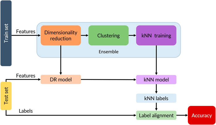
FIGURE 1. Flow diagram for the training and testing data. Features from the train set are reduced and clustered to generate labels (unsupervised learning). The resulting labels are then used to train a kNN model and an internal accuracy (kNN accuracy) is computed. The dimensionality reduction and kNN models are used to predict labels from the test set’s features and a real accuracy is computed by comparing the kNN labels with the ground truth labels (testing set labels).

3.1 Data

Two datasets are evaluated in this work. The first set of data that is analyzed is from the Tennessee Eastman Process (TEP), which was originally developed by Downs and Vogel and is often used for process control benchmarking (Downs and Vogel, 1993). TEP is a realistic, well-defined simulation with five unit operations (a reactor, condenser, separator, compressor, and stripper) that models four gaseous reactants competing in several reactions to produce two liquid products as well as an unwanted byproduct in the presence of an inert. The entire process has 41 measured variables and 12 manipulated variables for a total of 53 process variables. The complete dataset contains 3,365 samples, and an 80/20 training testing split was used.

The second set of data analyzed in this work is from an industrial pyrolysis reactor, which is a well-known industrial process unit that cracks heavy hydrocarbons into higher-value, lower molecular weight hydrocarbons. This dataset includes multiple modes of steady-state operation and exhibits process drifting due to equipment coking. The reaction takes place in a fired furnace, which is heated by burning fuel gas, as shown in Figure 2. These data come from a pyrolysis reactor that takes a feed of naphtha, mixes it with steam, and cracks it into ethylene at very high temperatures. This entire process has 27 variables, consisting of overall hydrocarbon flow, steam and hydrocarbon flow per tube, crossover temperatures and cracking temperatures per coil, the tube skin temperature, and the coil outlet temperature. Additional details about his process can be found elsewhere (Zhu et al., 2019). The complete dataset contains 1,482 samples and a 80/20 training testing split was used.

FIGURE 2

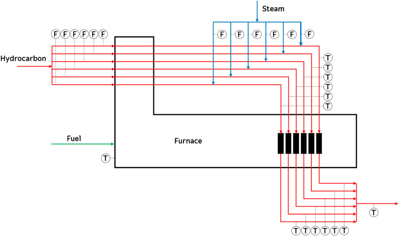
FIGURE 2. Pyrolysis Reactor process scheme.

3.2 Label alignment and automatic labeling performance

Since the clustering that will be learned by the kNN model was obtained in an unsupervised fashion, the labels assigned to the test set could be named differently than the ground truth label (i.e., “cluster 1” in the ground truth label is named “cluster 5” by the clustering algorithm, while containing the same data). Addressing this issue manually would be time-consuming and would hinder the evaluation of many ensembles and their hyperparameters. Hence, an automatic procedure was developed to align the labels predicted by the ensembles with the ground truth labels.

ALGORITHM 1

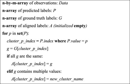
Algorithm 1. Align cluster labels with matching ground truth labels.

When the number of clusters generated is greater than the number of ground truth labels, the label alignment step will fuse some of the clusters as needed to get a match. If, on the other hand, the number of clusters is less than, the corresponding ensemble will misclassify the data, hence being penalized in the optimization step.

3.3 Automatic machine learning and optimization (non-dominated sorting genetic algorithm)

A challenge in the comparison of multiple dimensionality reduction and clustering ensembles is the great search space for the methods’ hyperparameters. Evolutionary algorithms have been shown to perform well for multi-objective hyperparameter optimization of machine learning models (Vishwakarma et al., 2019; Briceno-Mena et al., 2022b). Here, the selection of hyperparameters for each ensemble (see Table 1) is cast as a Mixed Integer Nonlinear Programming problem and solved using the Non-dominated Sorting Genetic Algorithm (NSGA-II) (Deb et al., 2002), as implemented by Pymoo (Blank and Deb, 2020). Additional details on NSGA-II and its implementation for hyperparameters tuning can be found elsewhere (Deb et al., 2002; Blank and Deb, 2020). A population size of 10 and a number of offspring 5 was used in all cases. For the supervised learning studies (when labels are available) the objective function aims to maximize the accuracy while minimizing the number of clusters. For the unsupervised learning studies (when labels are not available) the objective function aims to optimize the clustering metrics described in the following section. The output of the optimization step for this implementation is a Pareto front, in which candidate solutions are mapped according to the values of the individual objective functions so that the user can manually select the best solution among a small list of candidates.

TABLE 1

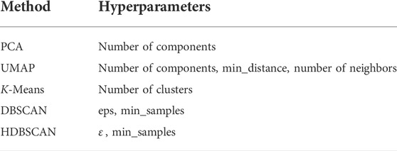
TABLE 1. Dimensionality reduction and clustering methods with their corresponding hyperparameters.

3.4 Clustering metrics

Unsupervised performance metrics provide information about the quality of the clustering ensemble. To investigate the correlation, if any, between these metrics and the performance of the ensembles in fault classification, three unsupervised performance metrics were tracked during the optimization of the ensembles: clustering, the silhouette score, the Davies-Bouldin Index, and the Calinski-Harabasz Index. The silhouette score (S-score) for a single sample represents how well it lies within the assigned cluster, as opposed to being close to 2 or more clusters (Rousseeuw, 1987). The silhouette score is calculated by the formula:

$s= \frac{b-a}{max\left(a,b\right)}(1)$

where $a$ is the mean distance between a sample and all other samples in its class and $b$ is the mean distance between a sample and all samples in the nearest other class. To calculate the silhouette score for a clustering result, we can find the mean silhouette score of all the samples. Good scores are closer to 1, where bad scores are closer to −1, indicating misclassification.

The Davies-Bouldin Index (DBI) evaluates the similarity between clusters and can be computed as (Davies and Bouldin, 1979):

$DBI= \frac{1}{k}{\displaystyle \sum _{i=1}^k{R}_{ij}} (2)$

Where

$R_{ij}= \frac{s_i+s_j}{d_{ij}}(3)$

The mean distance between each point and its cluster centroid is given by $s_i$, and the distance between two cluster centroids is given by $d_{ij}$. Lower values of DBI imply better clustering, with a minimum value of zero.

The Calinski-Harabasz Index (CHI) is defined by the formula (Caliński and Harabasz, 1974):

$s= \frac{tr\left(B_k\right)}{tr\left(W_k\right)}\times \frac{n_E-k}{k-1}(4)$

Where $k$ is the number of clusters, $n_E$ is the total number of samples, $tr\left(B_k\right)$ is the between-cluster variance, and $tr\left(W_k\right)$ is the within-cluster variance. Since the variance within the cluster is desired to be smaller than that among different clusters, a high CHI is preferred.

4 Results and discussion

4.1 Tennessee Eastman Process

Nine different ensembles were optimized for fault classification using the Tennessee Eastman Process (TEP) dataset using all 20 faults plus the 1 normal state. This dataset contains 81 observations from each of the 21 states, except fault number 6, which only contains 12 observations. Figure 3 shows the pareto front for the ensembles optimized for high accuracy and low number of clusters. The relationship between the accuracy and the number of clusters follows an exponential behavior, which means that above certain accuracy, the number of clusters would increase greatly with only small improvements in the performance of the ensemble. For this particular dataset, an inflection point is observed around 0.75 accuracy, where K-means clustering coupled with either UMAP or PCA shows good performance with a number of clusters around 45. This number of clusters could be associated with the identification of a transition region for each fault, resulting in at least two clusters (transition and new steady state) for each fault for a total of 40 well-defined regions. These results suggest that a kNN classifier combined with PCA for dimensionality reduction and K-means for clustering would produce a computationally efficient and reasonably accurate multi-mode classification ensemble with applications in process monitoring. On the other hand, obtaining a low dimensional space before the clustering step was not found to be a necessary condition to improve performance. However, it could be inferred that for K-means, going below 10 dimensions using PCA is detrimental, while UMAP could potentially allow a reasonable performance in lower dimensions, with the added benefit of being easier to visualize.

FIGURE 3

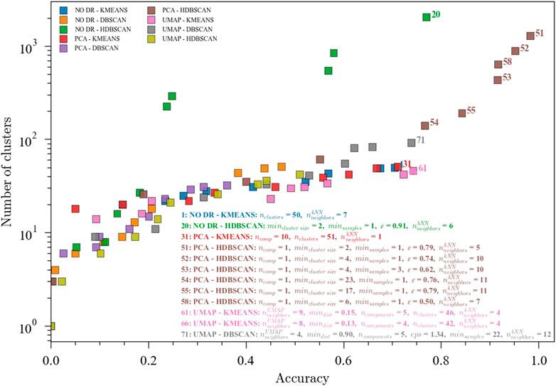
FIGURE 3. Pareto fronts for the multi-objective (accuracy and number of clusters) optimization of the ensembles. The hyperparameters for the accuracies above 0.70 are shown. Data from the Tennessee Eastman Process dataset with 20 faults. Ensembles: (1) NO DR-KMEANS, $n_{clusters}=50$, $n_{neighbors}^{kNN}=7$; (20) NO DR-HDBSCAN, $mi{n}_{cluster size}=2$, $mi{n}_{samples}=1$, $\epsilon =0.91$, $n_{neighbors}^{kNN}=6$; (31) PCA-KMEANS, $n_{components}=10$, $n_{clusters}=50$, $n_{neighbors}^{\mathit{kNN}}=\mathrm{1}$; (51) PCA-HDBSCAN, $n_{components}=1$, $mi{n}_{cluster size}=2$, $mi{n}_{samples}=1$, $\epsilon =0.79$, $n_{neighbors}^{kNN}=5$; (52) PCA-HDBSCAN, $n_{components}=1$, $mi{n}_{cluster size}=4$, $mi{n}_{samples}=1$, $\epsilon =0.74$, $n_{neighbors}^{kNN}=10$; (53) PCA-HDBSCAN, $n_{components}=1$, $mi{n}_{cluster size}=4$, $mi{n}_{samples}=3$, $\epsilon =0.62$, $n_{neighbors}^{kNN}=10$; (54) PCA-HDBSCAN, $n_{components}=1$, $mi{n}_{cluster size}=23$, $mi{n}_{samples}=1$, $\epsilon =0.76$, $n_{neighbors}^{kNN}=11$; (55) PCA-HDBSCAN, $n_{components}=1$, $mi{n}_{cluster size}=23$, $mi{n}_{samples}=1$, $\epsilon =0.79$, $n_{neighbors}^{kNN}=11$; (58) PCA-HDBSCAN, $n_{components}=1$, $mi{n}_{cluster size}=6$, $mi{n}_{samples}=1$, $\epsilon =0.50$, $n_{neighbors}^{kNN}=11$; (61) UMAP-KMEANS, $n_{neighbors}^{UMAP}=9$, $mi{n}_{dist}=0.15$, $n_{components}=5$, $n_{clusters}=46$, $n_{neighbors}^{kNN}=4$; (66) UMAP-KMEANS, $n_{neighbors}^{UMAP}=8$, $mi{n}_{dist}=0.13$, $n_{components}=4$, $n_{clusters}=42$, $n_{neighbors}^{kNN}=4$; (71) UMAP-DBSCAN, $n_{neighbors}^{UMAP}=4$, $mi{n}_{dist}=0.90$, $n_{components}=5$, $eps=1.34$, $mi{n}_{samples}=22$, $n_{neighbors}^{kNN}=12$.

The highest values for accuracy were observed with a much higher number of clusters, in particular the PCA-HDBSCAN ensemble. For these combinations, the optimizer finds a solution set where the average cluster size is very small—only containing a couple of data samples. The labels alignment step checks the predicted clusters for homogeneity and gives higher accuracy to homogenous clusters. Because this step assumes that predicted clusters can be combined if they are over-specified by the clustering algorithm, these smaller predicted clusters are often assigned perfectly to their matching ground truth label. In the context of DMKD, these solutions would require an engineer to manually combine several similar clusters which are artificially split, rendering a solution that is not very useful for exploratory data analysis. The presence of this type of solution reinforces the need for a multi-objective optimization problem that minimizes the number of clusters and finds a more meaningful solution.

In addition to the final accuracy and number of clusters, unsupervised metrics were tracked during the optimization for each ensemble to investigate if there exists a correlation that could then be exploited in situations where no labels are available. S-score and DBI (Figure 4) showed a strong correlation with accuracy for all of the ensembles, suggesting that aiming for better performance in these unsupervised metrics (high S-score and low DBI) could produce a reasonable starting point for unsupervised data analysis in the absence of labels to measure classification accuracy. It should be noted that for the PCA-K-means and NO DR-K-means ensembles, the DBI is not a strong predictor of accuracy. For the Calinski-Harabasz Index, a strong correlation with accuracy was found for No DR-K-means and PCA-K-means, but there seems to be no meaningful correlation for the other ensembles. In general, it is observed that unsupervised metrics could be good predictors of performance for fault detection ensembles. However, the metrics to be used are method dependent and should only be used as a starting point for the data analysis.

FIGURE 4

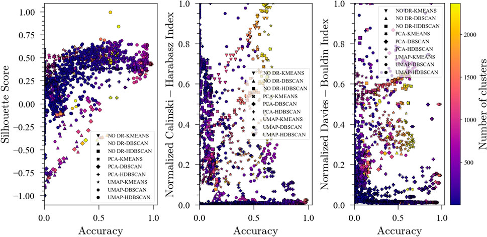
FIGURE 4. Evolution of the Silhouette Score, Davies-Bouldin Index and Calinski-Harabasz Index with accuracy during optimization for the Tennessee Eastman Process dataset with 20 faults.

Accuracies for the optimized ensembles with less than 50 clusters for the TEP dataset with all the faults were reasonable (around 0.75) but still low. However, it should be noted that the 21-way fault classification problem is considerably hard. In order to further explore the performance of the optimization framework, a reduced TEP dataset containing faults TEP01, TEP04, TEP07, TEP08, TEP10, TEP13 used. Faults 1, 4, and 7 are step change faults. Faults 8 and 10 are caused by random variation. Fault 13 is caused by a slow drift in the process. This selection is a good summary of the different types of faults present in the full TEP dataset. This dataset contains 481 observations from each of the 7 states (1 normal and 6 faults). Results for the selected TEP faults are shown in Figure 5 shows the performance of the optimization procedure for the nine ensembles. High accuracies were achieved with a lower number of clusters compared to the case with all the faults. These results are consistent with the hypothesis that a greater number of faults renders a more complex problem, for which extreme solutions are needed (i.e., a very high number of clusters).

FIGURE 5

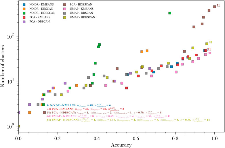
FIGURE 5. Pareto fronts for the multi-objective (accuracy and number of clusters) optimization of the ensembles. The hyperparameters for the accuracies above 0.70 are shown. Data from the Tennessee Eastman Process dataset with faults TEP01, TEP04, TEP07, TEP08, TEP10, and TEP13. Ensembles: (0) NO DR-KMEANS, $n_{clusters}=48$, $n_{neighbors}^{kNN}=6$; (20) NO DR-HDBSCAN, $mi{n}_{cluster size}=2$, $mi{n}_{samples}=1$, $\epsilon =0.91$, $n_{neighbors}^{kNN}=6$; (31) PCA-KMEANS, $n_{components}=40$, $n_{clusters}=48$, $n_{neighbors}^{kNN}=2$; (51) PCA-HDBSCAN, $n_{components}=1$, $mi{n}_{cluster size}=2$, $mi{n}_{samples}=1$, $\epsilon =0.79$, $n_{neighbors}^{kNN}=8$; (60) UMAP-KMEANS, $n_{neighbors}^{UMAP}=8$, $mi{n}_{dist}=0.69$, $n_{components}=4$, $n_{clusters}=39$, $n_{neighbors}^{kNN}=11$; (81) UMAP-HDBSCAN, $n_{neighbors}^{UMAP}=4$, $mi{n}_{dist}=0.19$, $n_{components}=4$, $mi{n}_{cluster size}=3$, $mi{n}_{samples}=5$, $\epsilon =0.34$, $n_{neighbors}^{kNN}=14$.

Figure 6 shows the evolution of the unsupervised metrics. As with the 20 faults, S-score and DBI are good predictors of the ensemble performance in the fault classification task while no clear patterns are observed for the CHI. These results, along with those for TEP with 20 faults, suggest that S-score and DBI could be used as objective functions to optimize the ensembles when labels are not available. An interesting observation regarding the evolution of DBI during optimization shown in Figure 6 is that for high DBI values with high accuracies, the number of clusters also increases. This could be helpful when optimizing for the unsupervised metrics since minimizing the DBI not only promotes high accuracy but also fewer clusters.

FIGURE 6

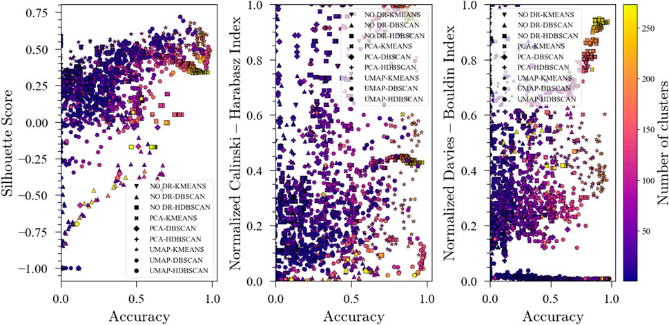
FIGURE 6. Evolution of the Silhouette Score, Davies-Bouldin Index and Calinski-Harabasz Index with accuracy during optimization for the Tennessee Eastman Process dataset with faults TEP01, TEP04, TEP07, TEP08, TEP10, and TEP13.

4.2 Pyrolysis reactor

An industrial dataset was also explored to assess the applicability of the methods here presented in a real plant setting. Results for fault classification in a pyrolysis reactor with three known states are shown in Figure 7. This dataset contains 76 observations from the first operating region, 28 observations from the second operating region, and 1379 observations from the third region. This imbalance is consistent with the normal operating modes of the process. With this being a simpler classification problem (only 3 classes), all ensembles achieved the maximum accuracy, with variability in the number of clusters. For this dataset, PCA for dimensionality reduction seems to have a better performance (same accuracy with fewer clusters) than UMAP. This could be explained by the global nature of the changes in the process. As discussed before, UMAP in general offers higher resolution which in this case is not needed. It is worth noting the importance of comparing multiple ensembles to find the more adequate combination for a particular application, and consequently the usefulness of an automated tuning framework which can ease the process of data analysis.

FIGURE 7

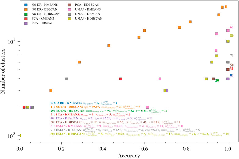
FIGURE 7. Pareto fronts for the multi-objective (accuracy and number of clusters) optimization of the ensembles. The hyperparameters for 1.0 accuracies are shown and one for each ensemble. Data from the pyrolysis reactor with 3 labeled faults. Ensembles: (0) NO DR-KMEANS, $n_{clusters}=5$, $n_{neighbors}^{kNN}=2$; (11) NO DR-DBSCAN, $eps=99.67$, $mi{n}_{samples}=3$, $n_{neighbors}^{kNN}=7$; (20) NO DR-HDBSCAN, $mi{n}_{cluster size}=97$, $mi{n}_{samples}=32$, $\epsilon =0.84$, $n_{neighbors}^{kNN}=11$; (31) PCA-KMEANS, $n_{components}=9$, $n_{clusters}=5$, $n_{neighbors}^{kNN}=2$; (40) PCA-DBSCAN, $n_{components}=3$, $eps=92.51$, $mi{n}_{samples}=5$, $n_{neighbors}^{kNN}=11$; (50) PCA-HDBSCAN, $n_{components}=12$, $mi{n}_{cluster size}=55$, $mi{n}_{samples}=42$, $\epsilon =0.19$, $n_{neighbors}^{kNN}=11$; (61) UMAP-KMEANS, $n_{neighbors}^{UMAP}=9$, $mi{n}_{dist}=0.78$, $n_{components}=4$, $n_{clusters}=13$, $n_{neighbors}^{kNN}=11$; (71) UMAP-DBSCAN, $n_{neighbors}^{UMAP}=5$, $mi{n}_{dist}=0.98$, $n_{components}=4$, $eps=5.01$, $mi{n}_{samples}=3$, $n_{neighbors}^{kNN}=5$; (71) UMAP-HDBSCAN, $n_{neighbors}^{UMAP}=8$, $mi{n}_{dist}=0.90$, $n_{components}=5$, $mi{n}_{cluster size}=17$, $mi{n}_{samples}=21$, $\epsilon =0.72$, $n_{neighbors}^{kNN}=15$.

The evolution of the unsupervised metrics during the optimization procedure for the pyrolysis process exhibited a similar behavior to that of the TEP. In general, a higher S-score and a lower DBI lead to better accuracy. Furthermore, for the CHI, some patterns are distinguishable with higher values being linked to higher accuracies.

4.3 Pyrolysis reactor: Unsupervised optimization

The results discussed in the previous sections for the optimization of ensembles for process monitoring are encouraging. However, this optimization requires the availability of labels to measure accuracy, which may not be the case for many industrial applications. Hence, the usefulness of unsupervised clustering metrics to predict the performance of the ensembles in the process monitoring task is highly valuable and was investigated. In this implementation, the S-score (maximize) and the DBI (minimize) were defined as objective functions (Figure 8). The Calinski-Harabasz Index was not included given the unclear results for the TEP. Figure 9 shows the pareto front for the pyrolysis reactor. The preferred solutions lie in the lower-right corner of the plot, with high accuracies and low DBI. In this region, the K-means (either combined with PCA or with no DR) appears as a good initial solution. It is worth noting, however, that if more resolution is needed (i.e., quick transition states between well slowly changing states) K-means may find difficulties in providing an adequate labeling and a density-based method such as DBSCAN might be better suited. In any case, the approach proposed here is only meant to give the user an initial solution that can be further improved either by inspection or by using additional methods. To visualize and compare these results, a SOM for the pyrolysis reactor dataset was produced (Figure 10). The initial solution for No DR-K-means resulted in 3 clusters which corresponded to the regions marked in the SOM (dark regions separated by bright lines). Further inspection of the SOM reveals a subregion near the higher right corner of the map (Figure 10C) which corresponds to the startup of the plant. Increasing the number of clusters in K-means from 3 to 4 readily reveals this cluster. This shows that the optimization of the ensembles using the unsupervised clustering metrics can be effective to provide an initial solution for the process monitoring task.

FIGURE 8

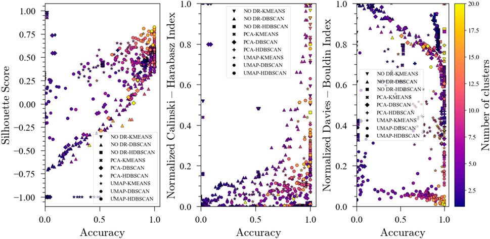
FIGURE 8. Evolution of the Silhouette Score, Davies-Bouldin Index and Calinski-Harabasz Index with accuracy during optimization for the pyrolysis reactor with 3 labeled faults.

FIGURE 9

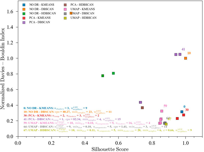
FIGURE 9. Pareto fronts for the unsupervised multi-objective (S-score and DBI) optimization of the ensembles. Data from the pyrolysis reactor without labels. (0) NO DR-KMEANS, $n_{clusters}=3$, $n_{neighbors}^{kNN}=9$; (10) NO DR-DBSCAN, $eps=80.27$, $mi{n}_{samples}=23$, $n_{neighbors}^{kNN}=11$; (30) PCA-KMEANS, $n_{components}=2$, $n_{clusters}=3$, $n_{neighbors}^{kNN}=2$; (41) PCA-DBSCAN, $n_{components}=1$, $eps=82.34$, $mi{n}_{samples}=4$, $n_{neighbors}^{kNN}=15$; (59) UMAP-KMEANS, $n_{neighbors}^{UMAP}=10$, $mi{n}_{dist}=0.10$, $n_{components}=5$, $n_{clusters}=16$, $n_{neighbors}^{kNN}=4$; (64) UMAP-DBSCAN, $n_{neighbors}^{UMAP}=9$, $mi{n}_{dist}=0.1$, $n_{components}=5$, $eps=1.41$, $mi{n}_{samples}=3$, $n_{neighbors}^{kNN}=14$; (67) UMAP-HDBSCAN, $n_{neighbors}^{UMAP}=10$, $mi{n}_{dist}=0.11$, $n_{components}=5$, $mi{n}_{cluster size}=20$, $mi{n}_{samples}=6$, $\epsilon =0.66$, $n_{neighbors}^{kNN}=9$.

FIGURE 10

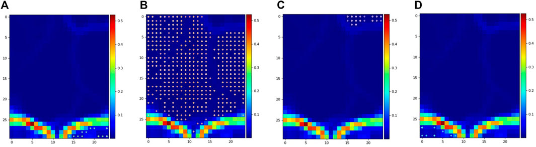
FIGURE 10. Projection of clusters over the self-organizing map for the pyrolysis reactor dataset using No DR-K-means (4 clusters).

5 Conclusion and future work

Performance of nine dimensionality reduction and clustering ensembles for process monitoring using a kNN classifier was investigated using an automatic Machine Learning framework based on a genetic algorithm. Results for a simulated data set and an industrial dataset showed that optimization of hyperparameters is possible and that this framework enables the fast exploration of ensembles and direct comparison, which is a useful tool for the unsupervised exploration of unlabeled plant data. In general, the number of clusters needed to represent the data distribution increases exponentially as the accuracy approaches 100%. However, reasonable accuracies can be obtained with fewer clusters. The effectiveness of unsupervised clustering metrics was explored by observing their evolution with accuracy during optimization. Results showed that Silhouette score and Davies-Bouldin index are strong predictors of the ensemble’s performances in the process monitoring task. For the Calinski-Harabasz index results are inconclusive. S-score and DBI were used for the optimization of ensembles for the industrial dataset (pyrolysis reactor), and it was shown that good initial results for the process monitoring task can be achieved in the absence of labeled data.

The research in this paper establishes the groundwork for several process monitoring research directions. First, more testing on the unsupervised optimization problem should be done. The goal of finding a good set of hyperparameters and methods to establish good clustering depends heavily on its ability to be reproduced, and the stochastic nature of some of these algorithms could make that difficult. Establishing a constant seeding in random number generation should be sufficient to reproduce the results, but some testing is required to confirm this. Another continuation is the expansion of this problem to other methodologies. One benefit of the automation of the optimization is that testing more methods becomes easier, so expanding the combinations to include more DR, clustering, and classification methods is natural. For this study, preprocessing normalization was done by subtracting features mean values from each term, but there are other options for techniques here as well. Additionally, the effect of distance metric selection could also be observed. For this study, only Euclidean distance is used for all similarity measures, but there are some other appropriate distance metrics such as the KL-divergence and Kantorovich distance that could be tested. Adding these selections as options in the optimization problem could lead to additional benefit in the clustering results.

Data availability statement

The original contributions presented in the study are included in the article/Supplementary Material, further inquiries can be directed to the corresponding author.

Author contributions

ZW: conceptualization, methodology, software, validation, investigation, formal analysis, data curation, writing—original, review and editing. LB-M: conceptualization, methodology, software, validation, investigation, formal analysis, visualization, writing—original, review and editing. MN: writing—original draft, resources, data curation, methodology, software. ES: writing—original draft, resources, data curation, methodology. JR: conceptualization, investigation, supervision, project administration, funding acquisition, writing—review and editing.

Conflict of interest

The authors declare that the research was conducted in the absence of any commercial or financial relationships that could be construed as a potential conflict of interest.

Publisher’s note

All claims expressed in this article are solely those of the authors and do not necessarily represent those of their affiliated organizations, or those of the publisher, the editors and the reviewers. Any product that may be evaluated in this article, or claim that may be made by its manufacturer, is not guaranteed or endorsed by the publisher.

References

Blank, J., and Deb, K. (2020). Pymoo: Multi-Objective optimization in Python. IEEE Access 8, 89497–89509. doi:10.1109/ACCESS.2020.2990567

CrossRef Full Text | Google Scholar

Briceno-Mena, L. A., Nnadili, M., Benton, M. G., and Romagnoli, J. A. (2022). Data mining and knowledge discovery in chemical processes: Effect of alternative processing techniques. Data-Centric Eng. 3, e18. doi:10.1017/dce.2022.21

CrossRef Full Text | Google Scholar

Briceno-Mena, L. A., Romagnoli, J. A., and Arges, C. G. (2022). PemNet: A transfer learning-based modeling approach of high-temperature polymer electrolyte membrane electrochemical systems. Industrial Eng. Chem. Res. 61, 3350–3357. doi:10.1021/acs.iecr.1c04237

CrossRef Full Text | Google Scholar

Buhmann, J., and Kühnel, H. (1993). Complexity optimized data clustering by competitive neural networks. Neural Comput. 5, 75–88. doi:10.1162/neco.1993.5.1.75

CrossRef Full Text | Google Scholar

Caliński, T., and Harabasz, J. (1974). A dendrite method for cluster analysis. Comm. Stats. - Theory &. Methods 3, 1–27. doi:10.1080/03610927408827101

CrossRef Full Text | Google Scholar

Chiang, L. H., Russell, E. L., and Braatz, R. D. (2000). Fault detection and diagnosis in industrial systems. Springer Science & Business Media.

Google Scholar

Davies, D. L., and Bouldin, D. W. (1979). A cluster separation measure. IEEE Trans. Pattern Analysis Mach. Intell. PAMI-1, 224–227. doi:10.1109/TPAMI.1979.4766909

PubMed Abstract | CrossRef Full Text | Google Scholar

Deb, K., Pratap, A., Agarwal, S., and Meyarivan, T. (2002). A fast and elitist multiobjective genetic algorithm: NSGA-II. IEEE Trans. Evol. Comput. 6, 182–197. doi:10.1109/4235.996017

CrossRef Full Text | Google Scholar

Downs, J. J., and Vogel, E. F. (1993). A plant-wide industrial process control problem. Comput. Chem. Eng. 17, 245–255. doi:10.1016/0098-1354(93)80018-I

CrossRef Full Text | Google Scholar

Hartigan, J. A., and Wong, M. A. (1979). Algorithm as 136: A k-means clustering algorithm. J. R. Stat. Soc. 28, 100–108. doi:10.2307/2346830

CrossRef Full Text | Google Scholar

He, Q. P., and Wang, J. (2007). fault detection using the k-nearest neighbor rule for semiconductor manufacturing processes. IEEE Trans. Semicond. Manuf. 20, 345–354. doi:10.1109/TSM.2007.907607

CrossRef Full Text | Google Scholar

Hotelling, H. (1933). Analysis of a complex of statistical variables into principal components. J. Educ. Psychol. 24, 417–441. doi:10.1037/h0071325

CrossRef Full Text | Google Scholar

Jimenez, L. O., and Landgrebe, D. A. (1998). Supervised classification in high-dimensional space: Geometrical, statistical, and asymptotical properties of multivariate data. IEEE Trans. Syst. Man. Cybern. C 28, 39–54. doi:10.1109/5326.661089

CrossRef Full Text | Google Scholar

Jolliffe, I. T. (1986). Principal component analysis. Springer-Verlag.

Google Scholar

Joswiak, M., Peng, Y., Castillo, I., and Chiang, L. H. (2019). Dimensionality reduction for visualizing industrial chemical process data. Control Eng. Pract. 93, 104189. doi:10.1016/j.conengprac.2019.104189

CrossRef Full Text | Google Scholar

Kohonen, T. (1990). The self-organizing map. Proc. IEEE 78, 1464–1480. doi:10.1109/5.58325

CrossRef Full Text | Google Scholar

McInnes, L., Healy, J., and Astels, S. (2017). Hdbscan: Hierarchical density based clustering. J. Open Source Softw. 2. doi:10.21105/joss.00205

CrossRef Full Text | Google Scholar

McInnes, L., Healy, J., and Melville, J. (2018). UMAP- uniform manifold approximation and projection for dimension reduction. arXiv, 1802.

Google Scholar

Pedregosa, F., Varoquaux, G., Gramfort, A., Michel, V., Thirion, B., Grisel, O., et al. (2011). Scikit-learn: Machine learning in Python. J. Mach. Learn. Res. 12, 2825–2830.

Google Scholar

Rousseeuw, P. J. (1987). Silhouettes: A graphical aid to the interpretation and validation of cluster analysis. J. Comput. Appl. Math. 20, 53–65. doi:10.1016/0377-0427(87)90125-7

CrossRef Full Text | Google Scholar

Tan, P. N., Steinbach, M., Karpatne, A., and Kumar, V. (2021). Introduction to data mining (2nd edition). Available at: https://www-users.cse.umn.edu/∼kumar001/dmbook/index.php.

Google Scholar

Vesanto, J., and Alhoniemi, E. (2000). Clustering of the self-organizing map. IEEE Trans. Neural Netw. 11, 586–600. doi:10.1109/72.846731

PubMed Abstract | CrossRef Full Text | Google Scholar

Vishwakarma, G., Haghighatlari, M., and Hachmann, J. (2019). Towards autonomous machine learning in chemistry via evolutionary algorithms. ChemRxiv. doi:10.26434/chemrxiv.9782387.v1

CrossRef Full Text | Google Scholar

Wagstaff, K., Cardie, C., Rogers, S., and Schrödl, S. (2001). Constrained k-means clustering with background knowledge. Icml 1, 577–584. doi:10.5555/645530.655669

CrossRef Full Text | Google Scholar

Zhu, W., Sun, W., and Romagnoli, J. (2018). Adaptive k-nearest-neighbor method for process monitoring. Industrial Eng. Chem. Res. 57, 2574–2586. doi:10.1021/acs.iecr.7b03771

CrossRef Full Text | Google Scholar

Zhu, W., Webb, Z. T., Mao, K., and Romagnoli, J. (2019). A deep learning approach for process data visualization using t-distributed stochastic neighbor embedding. Industrial Eng. Chem. Res. 58, 9564–9575. doi:10.1021/acs.iecr.9b00975

CrossRef Full Text | Google Scholar