Exploiting Trade-Off Criteria to Improve the Efficiency of Genetic Multi-Objective Optimisation Algorithms

The highly competitive nature of the chemical industry requires the optimisation of the design and exploitation of (bio-)chemical processes with respect to multiple, often conflicting objectives. Genetic algorithms are widely used in the context of multi-objective optimisation due to their overall straightforward implementation and numerous other advantages. NSGA-II, one of the current state-of-the-art algorithms in genetic multi-objective optimisation has, however, two major shortcomings, inherent to evolutionary algorithms: 1) the inability to distinguish between solutions based on their mutual trade-off and distribution; 2) a problem-irrelevant stopping criterion based on a maximum number of iterations. The former results in a Pareto front that contains redundant solutions. The latter results in an unnecessary high computation time. In this manuscript, a novel strategy is presented to overcome these shortcomings: t-domination. t-domination uses the concept of regions of practically insignificant trade-off (PIT-regions) to distinguish between solutions based on their trade-off. Two solutions that are located in each other’s PIT-regions are deemed insignificantly different and therefore one can be discarded. Additionally, extrapolating the concept of t-domination to two subsequent solution populations results in a problem-relevant stopping criterion. The novel algorithm is capable of generating a Pareto front with a trade-off-based solution resolution and displays a significant reduction in computation time in comparison to the original NSGA-II algorithm. The algorithm is illustrated on benchmark scalar case studies and a fed-batch reactor case study.

1 Introduction

To maintain a competitive position in the current worldwide market, companies need to operate their processes as optimally as possible with respect to different, often conflicting, objectives. These objectives can include for instance optimality with respect to societal, environmental and economical aspects. In such case, not just one optimal solution exists and decision makers need to resort to trade-off (or Pareto-optimal) solutions. The optimisation of a process with respect to different conflicting objectives is called a multi-objective optimisation problem (MOOP) and the solution of such a problem is the Pareto set or Pareto front, comprising all equally optimal trade-off solutions. Computing (an approximation of) this Pareto front is the main goal when solving a MOOP. The human decision maker will choose one optimal solution from the Pareto front as an operating point. It is desirable to produce a diverse Pareto set in a minimal computing time (Vallerio et al., 2015). MOOPs are mathematically challenging problems and are generally solved via the use of dedicated algorithms. The two major algorithm categories are scalarisation methods and vectorisation methods (Logist et al., 2010).

Scalarisation methods employ deterministic algorithms and translate the MOOP into a set of single objective optimisation problems (SOOPs) via the use of weight factors (Haimes et al., 1971; Das and Dennis, 1997, 1998; Messac et al., 2003; Marler and Arora, 2010; Logist et al., 2012). The SOOPs are then minimised independently from the other objectives. This renders one non-dominated solution for each SOOP. Sequentially solving the set of SOOPs eventually results in the calculation of several solutions that are expected to be located on the Pareto front (Logist et al., 2010). The most intuitive scalarisation method is the weighted sum method (Das and Dennis, 1997). It converts the MOOP into a SOOP by making a convex combination of the objectives with the use of weight factors $w_i$. Its main drawbacks are that points in the non-convex part of a Pareto front cannot be computed and an even spread of the weights $w_i$ does not necessarily produce an even spread of points on the Pareto front. More advanced scalarisation methods like normal boundary intersection (Das and Dennis, 1998) and enhanced normalised normal constraint (Messac et al., 2003) circumvent these drawbacks. Typically, deterministic gradient-based algorithms are used for solving the SOOPs generated by scalarisation methods. The advantage of these types of methods is that these can handle large numbers of decision variables and constraints. The major drawback of deterministic algorithms is that they incline to converge to local optima. Other drawbacks of some deterministic algorithms are that they cannot reach non-convex areas of the Pareto front or that these algorithms generate non-Pareto solutions (i.e., solutions that are not located on the Pareto front but are dominated by others) (Logist et al., 2010). Their major advantages are that they can be easily run computer wise, accompanied with a relatively short computing time.

Vectorisation methods use stochastic algorithms to solve a MOOP and tackle the MOOP as a whole (Bhaskar et al., 2000; Deb et al., 2002; Deb et al., 2005; Reyes-Sierra and Coello, 2006; Suman and Kumar, 2006; Jain and Deb, 2014). Vectorisation methods can be easily implemented and do not tend to converge to local optima, but are mostly unable to deal with complex constraints. Because all the objectives must be repeatedly compared, the algorithm can be time consuming when handling many-objective problems (i.e., multi-objective problems with four or more objectives). Thus, vectorisation methods are practically limited to low dimensional search spaces (Logist et al., 2010). A sub-field of the stochastic algorithms are the evolutionary algorithms (EA), on which the overall focus of this article will be. One of the main features of evolutionary multi-objective optimisation algorithms is that they are able to simultaneously generate multiple Pareto-optimal solutions (i.e solutions located on the Pareto front). This makes them an excellent choice to solve multi-objective optimisation problems, especially if the decision maker is interested in a diverse set of solutions. Additionally, EAs have no need for derivative information which makes them suitable for black box optimisation (Munoz Lopez et al., 2018; Yuen et al., 2018).

Early evolutionary algorithms were lacking elitism and had a high computational complexity. Elitism allows the algorithm to keep the best solutions of the previous iteration unchanged in the current one, which significantly increases the convergence speed of the algorithm. In order to maintain a decent spread in solutions, the user had to define a sharing parameter. However, the overall efficiency of the algorithm was highly dependent on the value of this sharing parameter. The lack of elitism of the first evolutionary algorithms prevented a fast convergence to the Pareto front. More contemporary evolutionary algorithms like non-dominated sorting genetic algorithm II (NSGA-II) resolved the shortcomings of the early algorithms (Deb et al., 2002). Non-dominated sorting genetic algorithm III (NSGA-III) is based on the framework of NSGA-II but was especially developed to handle many-objective problems (Deb and Jain, 2014). As in this article no many-objective problems will be discussed, the NSGA-III algorithm will not be further considered. Although both NSGA-II and NSGA-III were a substantial step in the right direction, numerous improvements can still be made.

The NSGA-II algorithm has already been subjected to numerous improvements or adaptions tailored for specific problems. These include, i.a., hybridising the NSGA-II algorithm with a gradient-based descent direction search to improve convergence, as presented by Yu et al., (2011) or introducing chaotic map models to improve the distribution of the initial random parent population, as presented by Liu et al., (2017). Controlled-NSGA-II, on the other hand, was developed as an answer on the potential over-emphasizing of NSGA-II on elitist solution, and was proposed by Deb and Goel (2001).

The overall goal of this article is therefore to point out some additional shortcomings of the widely popular NSGA-II algorithm and to propose solutions for these shortcomings by presenting a novel algorithm. The emphasis will be on two aspects: 1) the solution density in high and low trade-off Pareto areas, and 2) the introduction of a novel and problem-relevant stopping criterion.

When the decision maker switches between Pareto-optimal solutions, a trade-off will occur: the new Pareto-optimal solution will have gained in certain objectives and will have become less favourable with regard to others compared to the previously selected Pareto-optimal solution. Solutions located in high trade-off regions of the Pareto front display a significant trade-off amongst each other, i.e., switching between these solutions results in significant changes in the objective function values. These high trade-off solutions are of bigger interest to the decision maker than the low trade-off solutions, which are located in the low trade-off regions of the Pareto front (Mattson et al., 2004). Adapting the solutions’ resolution on the Pareto front, based on the trade-off, would result in less cluttered Pareto front, which in turn is more informative for the decision makers as it only displays solutions of interest. The decision makers can often quantify the trade-offs they deem to be significant for each objective function without needing to have prior knowledge on the shape of the Pareto front. Especially when the optimisation is considered of a process already operating in a non-optimal condition. In practise, changing the working point of a process often also introduces an extra cost as machinery might have to adapted, more full-time equivalents will required, etc. This knowledge often enables the decision makers to be able to quantify which minimum trade-off is required to make these changes worthwhile. For instance, when optimising the overall profit of a process and the current profit equals €100 per unit produced, a predicted profit gain of €1 will probably not trigger the decision makers to change the process accordingly, whereas a predicted profit gain of €10 probably would, resulting in a minimally required trade-off of 10.00% for that particular objective.

The second aspect this article will focus on, is improving the stopping criterion that is used. Most currently available genetic algorithms, NSGA-II included, employ an arbitrarily chosen default stopping criterion which has little relevance to the main goal of the multi-objective optimisation, i.e., generating Pareto-optimal solutions. The stopping criterion currently employed in NSGA-II consists of reaching a pre-defined number of iterations. As it is difficult for decision makers to assess upfront how many iterations will be needed to obtain a satisfactory Pareto front, a cautious stance is often assumed which, more often than not, results in the considerable over-estimation of the amount of iterations that are required. Especially for bigger optimisation problems, considering the optimisation of complex (bio-)chemical processes, and optimisation problems that are linked with process simulations, it is of the utmost importance that the amount of iterations that are required are kept to minimum to avoid the unnecessary loss of (computational) time. Genetic algorithms especially are extremely well-suited for optimising complex black-box problems. Several optimisation toolboxes already exploit this by providing decision makers with a suite of (adapted) genetic optimisation algorithms and an easy linkage between the optimisation platform and the simulation platform. Examples include the work by Ernst et al., (2017) and the in-house developed optimisation toolbox by Munoz Lopez et al., (2018).

The remainder of this article is structured as follows. Firstly, the mathematical formulation of a multi-objective optimisation problem is presented. Subsequently, the concept of evolutionary algorithms is introduced, followed by an in-depth discussion of NSGA-II, also addressing its major shortcomings. Next, the novel tDOM-NSGA-II is presented. Both algorithms will be applied to five scalar case studies (four bi-objective optimisation problems and one three-objective problems) and one dynamic benchmark case study, the Williams-Otto reactor (Williams and Otto, 1960). The obtained results are examined and an overall discussion is presented. To conclude, the main findings and contributions are summarised and perspectives for future work are presented.

2 Multi-Objective Optimisation Problems

The following multi-objective optimisation problem formulation is used throughout this article (Das and Dennis, 1997):

$\underset{\mathbf{x}\in C}{\text{min}}F\left(\mathbf{x}\right)=\left\{f_1\left(\mathbf{x}\right)\dots f_M\left(\mathbf{x}\right)\right\}(1)$

with:

$C=\left\{\mathbf{x}:\mathbf{h}\left(\mathbf{x}\right)=0;\mathbf{g}\left(\mathbf{x}\right)\le 0;\mathbf{a}\le \mathbf{x}\le \mathbf{b}\right\}(2)$

In Eq. 1$f_i:{\mathrm{ℝ}}^n\mapsto \mathrm{ℝ}$ is the ith objective function and $\mathbf{x}\in {\mathrm{ℝ}}^n$ represents the vector of optimisation variables. The set of constraints that have to be satisfied is denoted by C in Eq. 2, with $\mathbf{h}:{\mathrm{ℝ}}^n\mapsto {\mathrm{ℝ}}^{ne}$ the equality constraints, $\mathbf{g}:{\mathrm{ℝ}}^n\mapsto {\mathrm{ℝ}}^{ni}$ the inequality constraints and $\mathbf{a}$ and $\mathbf{b}$ being the respective lower and upper boundaries of the optimisation variables. Only the values of the optimisation variables that are part of C will provide a feasible solution of the optimisation problem. M stands for the number of objectives, n is the number of optimisation variables, $ne$ is the number of equality constraints and $ni$ is the number of inequality constraints (Das and Dennis, 1997).

A solution ${\mathbf{x}}^{\text{*}}$ of the MOOP is Pareto optimal or non-dominated if there exists no other solution $\mathbf{x}$ for which $F\left(\mathbf{x}\right)\le F\left({\mathbf{x}}^{\text{*}}\right)$, and additionally for this solution $\mathbf{x}$ at least one of the objectives $f_k\left(\mathbf{x}\right)<f_k\left({\mathbf{x}}^{\text{*}}\right)$ with $k\in \left\{1\dots M\right\}$. If there exists such a solution $\mathbf{x}$, then ${\mathbf{x}}^{\text{*}}$ is not Pareto optimal but dominated by $\mathbf{x}$. The Pareto front of an optimisation problem is the set of Pareto optimal solutions (Das and Dennis, 1997).

3 Evolutionary Algorithms

3.1 General Outline

An evolutionary algorithm (EA) is a population-based optimisation method which draws its basic philosophy from biological evolution. Mechanisms such as reproduction, selection of the fittest, mutation, etc. that are commonly linked to biological reproduction and evolution, are also found in an evolutionary algorithm (Back, 1996).

The first step of an EA consists of generating an initial random set of population members. In the context of solving a MOOP, these population members are feasible solutions of the MOOP. In a next step, the EA enters its main loop. The main loop of an EA starts with the generation of new offspring population members. These offspring population members are obtained by mutating and/or recombining (via a crossover) the parent population members of the previous generation of the main loop. In elitist algorithms, like NSGA-II, the offspring set of population members and the set of parent population members are merged into a combined set of population members. The fitness of the population members of the combined set is evaluated and these are subsequently sorted accordingly. The fitness of population members is determined by their level of convergence to the Pareto front and their contribution to the overall solution diversity. The level of convergence of a solution is assessed by sorting the whole population into their corresponding non-dominated fronts. The first non-dominated front contains all the population members that do not dominate each other but dominate other population members. The population members of the second non-dominated front are dominated by at least one population members of the first front, do not dominate each other, but dominate the population members of the third front and so on. Solutions’ contributions to the overall solution diversity is assessed by quantifying the average distance between consecutive solutions of the same non-dominated front. The last step of the main loop of an EA comprises of the selection of the fittest population members. The other population members are discarded. The acquired set of fittest population members forms the parent population members set for the next generation of the main loop. This process is repeated until a termination parameter is satisfied. Because after each generation only the fittest population members are retained, the population members will eventually converge to the most optimal scenario, i.e., the Pareto front (Knowles and Corne, 1999; Deb et al., 2002). This process is graphically displayed in Figure 1.

FIGURE 1

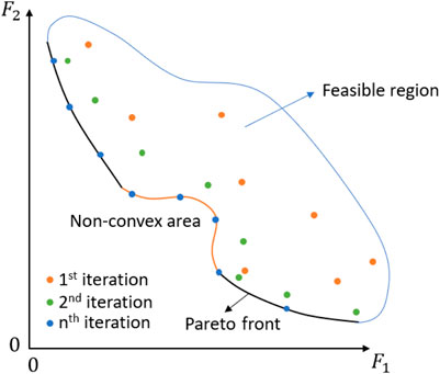
FIGURE 1. General representation of a solving method for multi-objective optimisation problems based on an evolutionary algorithm. Both objective functions are minimised.

The solutions displayed in Figure 1 as the solutions of the first iteration, are the randomly generated solutions within the feasible space. Via subsequent selection, mutation and crossover actions during the following generations, the generated solutions move closer to the Pareto front. The solutions of the final nth iteration are located in the close proximity of the Pareto front. Non-convex areas of the Pareto front can be reached as well as convex areas. Additionally, while scalarisation methods tend to converge to local optima, evolutionary algorithms generally produce global optima of the concerned MOOP.

The high computational complexity of the early evolutionary algorithms was a consequence of the used non-dominated sorting approach. Computational complexities reached as high as $O\left(M{N}^3\right)$ (with M the number of objectives and N the size of the solution-population). These computational complexities were reduced in newer algorithms via the use of less complex sorting approaches. Other improvements seen in these algorithms, are their use of elitism and crowded comparison. The sharing parameter of the early algorithms was replaced by the crowded comparison approach to keep enough diversity amongst the solutions in a set (Deb et al., 2002).

Thanks to these three major improvements, new algorithms like NSGA-II and NSGA-III have grown very popular and are commonly used. Nonetheless, further improvements can still be made. For instance, it would be desirable to create a Pareto front with a trade-off based adaptable solution resolution. The Pareto front can namely be subdivided in areas containing high trade-off solutions and areas containing low trade-off solutions. High trade-off solutions are of bigger interest for the decision maker and are located on steep segments of the Pareto front while solutions with a low trade-off are located on the flat sections (Hashem et al., 2017).

In the following, the trade-offs of generated solutions will be investigated more deeply and the question on how to eventually obtain a Pareto front with an adaptive resolution will be addressed. Firstly, the NSGA-II algorithm is thoroughly discussed.

3.2 NSGA-II

3.2.1 Algorithm Outline

The flow sheet of the NSGA-II algorithm is depicted in Figure 2. NSGA-II is a multi-objective evolutionary algorithm developed as an answer to the shortcomings of the early EAs. It uses non-dominated sorting and sharing, like all other EAs, but it was one of the first EAs to employ elitism and crowded comparison. NSGA-II uses a fast non-dominated sorting mechanism which allowed the reduction of the computational complexity of the algorithm to $O\left(M{N}^2\right)$ (Deb et al., 2002).

FIGURE 2

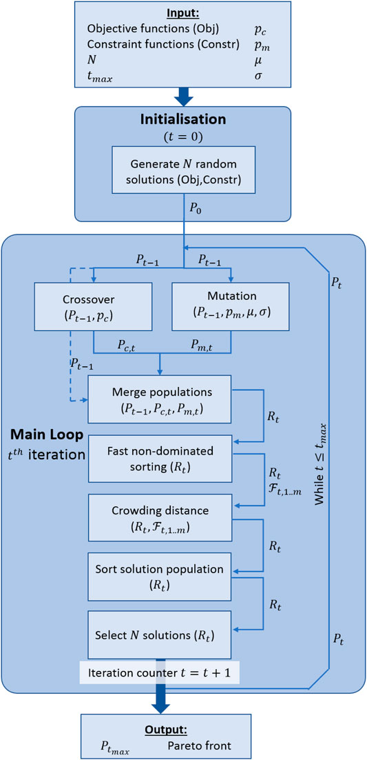
FIGURE 2. Flow sheet of the NSGA-II algorithm.

During the first iteration, N initial random solutions are generated and are added to the parent set P₀. The initial random parent solutions are used to generate the offspring set $Q_1$ ($Q_1=P_{c,1}\cup P_{m,1}$ and $\left|Q_1\right|=N$). Offspring solutions are achieved via recombinations and mutations of the solutions in the parent set (Deb et al., 2002).

Considering the t-th generation of the algorithm, the elitist step of the NSGA-II algorithm consists of merging the parent set $P_{t-1}$ and the corresponding offspring set Q_t into a combined population R_t, with $\left|R_t\right|=2N$. This enables the algorithm to retain the fittest solutions of the previous generation unchanged in the current one. All the $2N$ solutions of the combined population are subsequently sorted in their corresponding non-dominated fronts and their crowding distances are calculated. Then, based on the rank of the non-dominated front to which they belong and their crowding distance, only the best N solutions are retained. Solutions that are located in the first few non-dominated fronts and have a high crowding distance are favoured. These solutions form the parent set P_t, i.e., the parent set of the $\left(t+1\right)$-th iteration. The iteration process is repeated until a maximum number of iterations is reached (Deb et al., 2002). Note that during the solution selection process, the fact whether or not solutions are of interest to the decision maker is not taken into account. Moreover, there is no possibility for the decision maker to provide any prior knowledge or preferences to the algorithm.

To solve a MOOP using NSGA-II, the number of iterations, the size of the solution population and the conventional EA-parameters, like the crossover probability and mutation probability, must be pre-defined by the user. For more details on the different steps of the algorithm, the interested reader is referred to (Deb et al., 2002; Deb et al., 2005; Jain and Deb, 2014; Valadi and Siarry, 2014; Liagkouras and Metaxiotis, 2017).

The stopping criterion used in NSGA-II is a default stopping criterion which is commonly used in other evolutionary algorithms as well: when a pre-defined number of iterations $t_{max}$ are reached, the algorithm is stopped. However, this stopping criterion has no relevance to the optimisation problem itself, while it does not take the quality of the solutions into account. Under-estimating the number of iterations required will result in a poor solution convergence, whereas an over-estimation will result in wasted computational time. A problem-relevant stopping criterion can be used to assess the performance of the optimisation algorithm and save computational time. Marti et al., (2016) mention that in case of evolutionary optimisation algorithms, a global stopping criterion that assesses the algorithm’ performance can become as complicated as the optimisation problem itself. Additionally, they point out that although the need for a problem-relevant stopping criterion has been previously frequently suggested as a research need, it has not received much attention in research concerned with the development of evolutionary algorithms. Most evolutionary algorithms bypass the need of developing a problem-relevant stopping criterion by resorting to the already mentioned default, but problem-irrelevant, stopping criterion. Marti et al., (2016) have introduced a novel global stopping criterion for evolutionary optimisation algorithms, which is based on information gathering techniques. When developing the stopping criterion, Marti et al., (2016) especially focussed on many-objective optimisation problems. A simpler, yet still problem-relevant stopping criterion will be presented in section 3.3.2, with a focus on low-dimensional optimisation problems.

3.2.2 Shortcomings

Based on the discussions above, two major shortcomings of the NSGA-II algorithm can be identified:

1. The solution selection process does not take into account if solutions are of interest to the decision maker. The latter has, additionally, no possibility to provide the algorithm with prior knowledge and/or solution preferences.

2. As a result of a problem-irrelevant stopping criterion (reaching a pre-defined number of iterations), a large part of the computational time will be uselessly spent on the continuation of the iteration process, even once all solutions have converged to the Pareto front.

Considering the shortcomings mentioned above, the main objective of this article is to present a novel genetic algorithm that is capable to assess the added value of solutions to the decision maker. This will done based on their mutual trade-off. Additionally, the novel algorithm will be equipped with a problem-relevant stopping criterion to avoid the unnecessary continuation of the optimisation process once all solutions have converged sufficiently.

3.3 tDOM-NSGA-II: Exploiting Trade-Off to Improve Efficiency

The tDOM-NSGA-II algorithm is developed to remedy the major shortcomings of the constrained NSGA-II algorithm. The main focus during the development of the tDOM-NSGA-II algorithm was to introduce a problem-relevant stopping criterion in order to avoid unnecessary excess iterations. Due to their design features, genetic algorithms are widely used in the context of complex black-box optimisation problems as, amongst others, they do not require derivative information. These black-box optimisation problems are often coupled with process simulators to generate solutions (i.e., simulate the process’s response on the proposed controls and settings in order to calculate the objective costs). In this scenario, the generation of solutions becomes the computationally expensive step, rather than the optimisation itself. Reducing the number of solutions that have to be generated becomes the main focus in the context of these complex optimisation problems. Therefore, during the development of the tDOM-NSGA-II, the main focus was on developing a genetic algorithm (using the original NSGA-II structure) that can assess if solutions have converged sufficiently and the optimisation process can be stopped, so that excess iterations are avoided. The fact that the proposed stopping criterion requires more solution comparison per iteration, is point not considered as an issue, as the anticipated significant decrease in iterations required would vastly outweigh the added computational cost due to the extra comparison required.

Additionally, the tDOM-algorithm is capable to distinguish between solutions based on their trade-off. This is achieved by the introduction of regions of practical insignificant trade-off (PIT-regions). If a solution is located in the PIT-region of another solution, both solutions are not considered to be significantly different by the decision maker. The crowdedness of the PIT-region of a solution is thus measure for its trade-off. The less crowded the PIT-region of a solution is, the higher its trade-off. The density of the PIT-region of a solution is accordingly introduced as a second crowding distance, making it an additional selection parameter.

The problem-relevant stopping criterion is based on the same concept by extrapolating it to the entire solution population: if two subsequent solution populations are entirely located in each others PIT-regions, they are not considered to be significantly different from one another by the decision maker. If this is the case, no significantly different solutions have been generated. As the framework of the NSGA-II algorithm is used as the backbone structure of the tDOM-NSGA-II algorithm, elitism is ensured. This implies that with evolving iterations, selected solutions are at least equally well converged and diverse as the solutions selected during the previous iteration. Therefore, once the algorithm starts repeatedly generating solutions that display little differences with respect to the previous solution generation, it can be concluded that the solutions have converged to the Pareto front. The concept of PIT-regions, or t-domination, is used in the context of the tDOM-NSGA-II algorithm to quantify the point when the difference between two subsequent solution generations become negligibly small and the algorithm can be terminated.

Hashem et al., (2017) already presented the idea of using the trade-off of solutions as a stopping criterion. In their divide and conquer scheme for deterministic algorithms, the exploration of a certain area of the Pareto front is ceased if the generated solution no longer displays the required trade-off or distribution. The tDOM-algorithm, which is presented in the remainder of this section, adapts the concept stated above to genetic algorithms.

In the remainder of this section, the novel tDOM-algorithm is presented. Firstly, the concepts PIT-region and t-domination are introduced. Subsequently, the trade-off function is presented which enables the algorithm to select solutions based on their trade-off and generate a trade-off based algorithm termination parameter.

3.3.1 PIT-Region: Trade-Off as a Second Crowding Distance

The trade-off $\text{Δ}t$ and distribution $\text{Δ}r$ of a solution p can be seen as properties imposed on the spatial distribution of other solutions around solution p, and show therefore great resemblances to the crowding distance of a solution, as used in NSGA-II. The crowding distance of a solution is defined as the average length of the edges of the cuboid formed around the concerned solution, with its neighbouring solutions as vertices. Because the desired solution trade-off $\text{Δ}t$ and distribution $\text{Δ}r$ are generally different for each objective function, the spatial form that they describe will often be much more complicated than a cuboid. Mattson et al., (2004) presented in this respect the region of practically insignificant trade-off, or the PIT-region. The PIT-region of a solution is depicted in Figure 3 for a bi-objective optimisation problem. Solutions that are located in the PIT-region of a solution p (red solutions) have no significant trade-off in regard to solution p and also to do not contribute to the overall solution diversity. They render no added value to the solution population and can therefore be discarded. The solutions located outside of the PIT-region of the concerned solution p are kept in population (green solutions).

FIGURE 3

FIGURE 3. Graphical representation of the PIT-region of a solution p for an optimisation problem with normalised objectives ${F^{\prime }}_1$ and ${F^{\prime }}_2$ [adapted from Mattson et al., (2004)].

The PIT-region, as presented by Mattson et al., (2004) has a cross-like shape in case of a bi-objective problem. The PIT-region presented by Mattson et al., (2004) only consisted out of the shaded sections. Because in the presented trade-off function, the trade-off and distribution of solutions will be determined one non-dominated front at a time, the PIT-region can be simplified to a complete cross, built up out of rectangles circumventing the concerned solutions. Solutions that are located in sections 1) or 2) of the PIT-region will be part of a lower or higher non-dominated front respectively. As already mentioned, note that the dimensions of the PIT-region, defined by $\text{Δ}t$ and $\text{Δ}r$, are not necessarily the same for each objective.

Mattson et al., (2004) used the PIT-region to reduce the size of a initially large solution population to eventually obtain two population sets: one set P₁ that contains all the discarded solutions and another set P₂ consisting out of the selected solutions that meet the required trade-off $\text{Δ}t$ and distribution $\text{Δ}r$. For this purpose, all the solutions are sorted in ascending order according to the objectives. Subsequently the solutions are visited in ascending order and the PIT-region is constructed around the concerned solution. While the visited solution is allocated to the population set P₂, all the solutions that are located in its PIT-region are discarded and are allocated to population set P₁. The discarded solutions are not visited and their PIT-region is therefore not constructed.

The main disadvantage of such an a posteriori selection step however is that this method requires a large number of solutions, of which a substantial fraction is discarded at the end of the selection process. Removing those solutions from the population set simultaneously implies that a large amount of computing time is used to generate useless solutions. To avoid this, the trade-off of a solution is introduced as an inherent solution property (like its objective cost, optimisation variables, etc.) in the tDOM-algorithm, based on which it can be sorted. The tDOM-algorithm constructs the PIT-region of all the generated solutions, one non-dominated front at a time, and assess the solution density of each PIT-region. The number of solutions located in the PIT-region of a concerned solution p is defined as its trade-off counter. The lower the value of this trade-off counter, the higher the trade-off of the concerned solution p is. Accordingly, during the sorting and selection step of the tDOM-algorithm, the solutions are additionally sorted in ascending order based on their trade-off counter. This results in emphasising solutions with a sparse PIT-region or with a high trade-off, a high crowding distance and a low non-dominated rank. After each iteration step of the tDOM-algorithm, only the N fittest solutions are selected for the parent set of the next iteration, eventually resulting in a solution population which largely consist out of diverse, non-dominated solutions with high trade-offs.

3.3.2 t-Domination: Trade-off as a Stopping Criterion

In the previous section, the concept of the PIT-region and how the trade-off of a solution can be used as a second crowding distance, was introduced. Up until this point, the minimal required trade-off $\text{Δ}t$ and distribution $\text{Δ}r$ have only been used as an additional crowding distance or diversification measure. The trade-off of solutions can, however, also be used as a stopping criterion. In order to do so, two additional inherent properties of the solution must be considered. In a first instance, the algorithm must be able to determine if a concerned solution is generated in the current iteration or in the previous one. The second additional inherent solution property is used to determine if the tDOM-algorithm can be stopped. To explain how the trade-off of a solution is used as stopping criterion, the concept of t-domination is introduced in the remainder of this section. For the ease of formulation, solutions that are generated via a tDOM-algorithm, will be further denoted as tDOM-solutions.

The concept of non-domination or Pareto-optimality has been mathematically introduced in Section 2. As a reminder: a solution $\mathbf{x}$ is non-dominated or Pareto-optimal if there exists no solution ${\mathbf{x}}^{\ast }$ for which for all $i\in \left\{1,\dots ,M\right\}:f_i\left({\mathbf{x}}^{\ast }\right)\le f_i\left(\mathbf{x}\right)$ and there exists at least one $i\in \left\{1,\dots ,M\right\}:f_i\left({\mathbf{x}}^{\ast }\right)<f_i\left(\mathbf{x}\right)$ with $f_i,i\in \left\{1,\dots ,M\right\}$ the M objective function of the concerned optimisation problem. Figure 4A graphically represents the concept of non-domination in case of a bi-objective problem. Based on the above non-domination definition, solution p₁ is dominated by solution q₄. q₄ is therefore a non-dominated solution. t-domination however also takes the PIT-region of the solution into account. A solution z is t-non-dominated if there exists no solution ${\mathbf{z}}^{\ast }$ for which $\forall i\in \left\{1,\dots ,M\right\}:f_i\left({\mathbf{z}}^{\ast }\right)\le f_i\left(\mathbf{z}\right)$ and $\exists i\in \left\{1,\dots ,M\right\}:f_i\left({\mathbf{z}}^{\ast }\right)<f_i\left(\mathbf{z}\right)$ and ${\mathbf{z}}^{\ast }\notin PIT\left(\mathbf{z}\right)$, with $f_i,i\in \left\{1,\dots ,M\right\}$ the M objective function of the concerned optimisation problem. t-domination is graphically represented in Figure 4B in case of a bi-objective problem. Although q₂ dominates p₁, it does not t-dominate p₁ while it is located in the PIT-region of p₁. q₁ on the other hand does t-dominate p₁, and is therefore t-non-dominated.

FIGURE 4

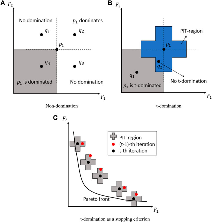
FIGURE 4. Graphical representation of non-domination (A), t-domination (B) and t-domination as a stopping criterion (C) in case of a bi-objective problem.

In section 3.3.1, it was mentioned that if a solution q is located in the PIT-region of another solution p, there is no significant difference between the two solutions. Because solution q does not display the required trade-off $\text{Δ}t$ or distribution $\text{Δ}r$ in comparison to solution p, it does not contribute to the diversification of the solution population, nor does it represent a significantly different process design than solution p. There is therefore no need of keeping q in the solution population and it can be discarded or downgraded.

If the concept of t-domination is extended to the whole solution population, it can be turned into a stopping criterion: if all the solutions of two subsequent solution populations are located in each others PIT-regions, there is no significant difference between the two populations and therefore the algorithm, or iteration process, can be stopped. This is graphically represented in Figure 4C. Because all the solutions of the (t − 1)-th iteration are located in the PIT-regions of the solutions of the t-th generation, the algorithm will be stopped because no new t-non-dominated solutions have been created. The black solutions of the t-th generation represent thus the final solution population.

The two concepts presented above are incorporated in the tDOM-algorithm in the form of a trade-off function, which is introduced in the next section.

3.3.3 Trade-Off Function

The presented trade-off function has a dual function. Mainly it is used to enable the tDOM-algorithm to sort and select solutions based on their trade-off. Just like solutions with a low crowding distance are disfavoured and downgraded during the selection procedure, solutions with a crowded PIT-region are disfavoured as well. The main functionality of the trade-off function is to quantify the amount of solutions in the PIT-region of a concerned solution. The introduced trade-off counter of a solution amounts to the number of solutions that are located in the PIT-region of the concerned solution. The more crowded the PIT-region of a solution is, the higher its trade-off counter will be. As a result of the cross-like shape of the PIT-region, solutions that are located in high trade-off areas of the Pareto front, i.e., steep segments and knees, will have a sparsely crowded PIT-region and their trade-off counter will therefore amount to a low value. Solutions located in the flat, low trade-off areas of the Pareto front on the other hand, will have a densely crowded PIT-region and their trade-off counter will amount to a high value.

Additionally the trade-off function is used to generate a termination parameter. It is opted to make this parameter an inherent solutions property, in the form of a logical value. If the termination parameters of all the solutions of a certain population are set to $\mathtt{t}\mathtt{r}\mathtt{u}\mathtt{e}$, the algorithm can be stopped. In order to determine the logical value of this termination parameter, the solutions of two subsequent population must be compared with one another. Because this is a computational expensive step, this is only done when ${\mathrm{ℱ}}_1\ge N$ or fraction of Pareto-optimal solutions (FPOS) $\ge$ 1. Because the trade-off function is executed before the N fittest solutions are selected, it is possible that the first non-dominated front contains more than N non-dominated solutions. The pseudo code of the trade-off function is presented in Algorithm 1.

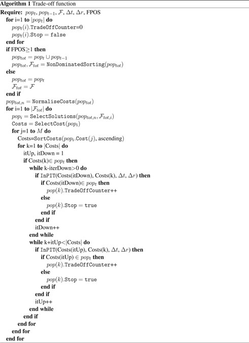
The trade-off function requires the current solution population $po{p}_t$, which is sorted in its non-dominated fronts $\mathrm{ℱ}$, the solution population generated during the previous iteration $po{p}_{t-1}$, the desired trade-off $\text{Δ}t$ and distribution $\text{Δ}r$, pre-defined by the decision maker, and the FPOS value of the current solution population. For the sake of clarity it is assumed that $\text{Δ}t$ and $\text{Δ}r$ have the same value for all the M objective functions. In a first instance the trade-off counters of all the solutions in $po{p}_t$ are reset to zero and their termination parameters are set to $\mathtt{f}\mathtt{a}\mathtt{l}\mathtt{s}\mathtt{e}$.If FPOS $\ge$ 1, the current solution population $po{p}_t$ and the solution population of the previous iteration are merged into the total solution population $po{p}_{tot}$. $po{p}_{tot}$ is subsequently sorted into its non-dominated fronts ${\mathrm{ℱ}}_{tot}$. This step is only done if FPOS $\ge$ 1, because the non-dominated sorting step of the obtained $po{p}_{tot}$ solution population will be computationally expensive, while it contains $3N$ solutions. If FPOS $<$ 1, $po{p}_t$ and $\mathrm{ℱ}$ are redefined as $po{p}_{tot}$ and ${\mathrm{ℱ}}_{tot}$ respectively for the sake of conformity. While $\text{Δ}t$ and $\text{Δ}r$ are disclosed as percentages, the objective costs of all the solutions in $po{p}_{tot}$ are normalised, rendering the normalised solution population $po{p}_{tot,n}$.The trade-off counter of the solutions is determined at a rate of one non-dominated front at a time. A new solution population $po{p}_i$ is constructed for the ith non-dominated front, which contains all the solutions that are allocated to this front. The objective costs of the solutions in $po{p}_i$ are clustered in the $M\times \left|po{p}_i\right|$ objective costs matrix, $Costs$. One column of $Costs$ contains all the objective costs of one solution and can be considered as the column vector in the objective space between the objective space origin and the solution. The trade-off function continues by sorting the column vectors of $Costs$ in ascending order according to the concerned objective of the optimisation problem. Subsequently, for each k-th column vector of the sorted objective cost matrix $Costs$, which is part of the current solution population $po{p}_t$, it is determined if the neighbouring objective costs, both in ascending en descending order according to the concerned objective, are located in its PIT-region. If this is the case, and the concerned neighbouring solutions is also part of the current solution population $po{p}_t$, the trade-off counter of the solution corresponding with the objective costs in the k-th column vector, is incremented by 1. If however the concerned neighbouring solution is part of $po{p}_{t-1}$ (which can only occur if FPOS $\ge$ 1), the termination parameter of the solution corresponding with the objective costs in the kth column vector is set to $\mathtt{t}\mathtt{r}\mathtt{u}\mathtt{e}$.Subsequently in the tDOM-algorithm, the trade-off counter is used as an additional sorting parameter. Ahead of sorting the solutions of the combined solution set $R_t$ according to their crowding distance and non-dominated rank, they are sorted according to their trade-off counter in ascending order (see 3.3.5). This result in emphasising solutions with a sparsely crowded PIT-region. Because the dimension of the PIT-region of a solution is not only dependent on a desired objective trade-off but also on a minimal solution diversity requirement, solution diversity will be more emphasised in the tDOM-algorithm.

3.3.4 Applicability of the t-domination Concept

In this paper, the concept of t-domination is only applied to the NSGA-II algorithm. This is done because the NSGA-II algorithm is one of the most widely used population-based optimisation methods. Note that this is also applicable to the NSGA-III algorithm which is derived from the NSGA-II algorithm. Other population-based optimisation methods, like Strength Pareto Evolutionary Algorithm (SPEA) (Zitzler and Thiele, 1999), Interactive Adaptive-Weight Genetic Algorithm (IAWGA) (Lin and Gen, 2009), and Pareto-Archived Evolutionary Strategy (PAES) (Knowles and Corne, 1999), can be equipped with the presented t-domination concept as a stopping criterion and/or selection parameter.

3.3.5 Algorithm Outline

The tDOM-algorithm requires, just like the constrained NSGA-II algorithm, the objective functions (Obj), the constraints (Constr), the desired population size N, the maximum number of iterations $t_{max}$ and the genetic operation parameters $p_m$, μ, σ, and $p_c$. Additionally the tDOM-algorithm requires the trade-off parameter $\text{Δ}t$ and the distribution parameter $\text{Δ}r$. The pseudo code of the tDOM-algorithm is presented in Algorithm 2.

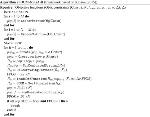
The initialisation step consists of the generation of the random initial solution population. In order to guarantee that the initial population already displays an adequate solution diversity, the anchor points are included in the initial population. These are the individual minimisers of the concerned objective functions, which are determined upfront. The $N-M$ remaining solutions are randomly generated within the feasible space which is defined by the constraint functions.The main loop starts with the generation of new offspring solutions via a mutation and crossover step of the solution population of the previous iteration. Just like in NSGA-II, the elitist step of the tDOM-NSGA-II algorithm is accomplished by merging the set of offspring solutions with the solution population of the previous iteration. The obtained combined solution set $R_{it}$ is sorted into its non-dominated fronts ${\mathrm{ℱ}}_{it}$, after which the crowding distance of all the solutions of $R_{it}$ is determined. Up until this point, the tDOM-NSGA-II algorithm is the complete analogue of the NSGA-II algorithm (the anchor points not taken into account).The NSGA-II algorithm would at this point continue by sorting the solutions of $R_{it}$ according to their crowding distance and non-dominated front. The tDOM-NSGA-II algorithm however utilises three fitness parameters: the non-dominated rank, the crowding distance, and the solution trade-off. The trade-off of a solution, or more specifically its trade-off counter, is determined with the trade-off function (see 3.3.3). This algorithm step is preceded with the calculation of the FPOS value of the $R_{it}$ solution population. If FPOS $<$ 1, then the trade-off function is only used to determine the trade-off counter of the solutions of $R_{it}$. All the termination parameters of the solutions of $R_{it}$ are set to $\mathtt{f}\mathtt{a}\mathtt{l}\mathtt{s}\mathtt{e}$. If however FPOS $\ge$ 1, the trade-off function is additionally used to determine the termination parameters of the solutions in $R_{it}$ (see 3.3.3).In order to sort the solutions of $R_{it}$ according their fitness, tDOM-NSGA-II uses a tDOM-sort function. $R_{it}$ can be considered as an array containing solutions in a certain sequence. In a first instance, the solutions are sorted in ascending order according to their trade-off counter. Thus solutions with a high trade-off (i.e., solutions with a sparsely crowded PIT-region) are sorted in the highest positions of the population array. Subsequently the obtained array is sorted in descending order according to the crowding distance and finally in ascending order according to the non-dominated rank. Solutions with a low non-dominated rank and a high trade-off and crowding distance are sorted in the top positions of the population array. Selecting the N fittest solutions is now simplified to selecting the first N solutions of the obtained population array.The last step of the tDOM-NSGA-II main loop consists of updating the non-dominated fronts of the generated population $pop$. If FPOS = 1 and all the termination parameters of the solutions in $pop$ are set to $\mathtt{t}\mathtt{r}\mathtt{u}\mathtt{e}$, the main loop is terminated.

4 Benchmark Case Studies and Methods

To test the performance of the developed algorithm, both NSGA-II and tDOM-NSGA-II have been applied to five benchmark case studies have been: four scalar bi-objective case studies and one scalar three-objective case study. The Williams-Otto reactor case study has been implemented to illustrate the use of the algorithm for the optimisation of dynamic chemical processes. These case studies are presented below. MATLAB R2018b is used as the optimisation platform and is run on a 64-bit Windows 10 system with an Intel Core i5-8500 CPU @ 3.00 GHz processor and 16 GB of RAM installed.

4.1 Bi-objective Case Studies

The bi-objective case studies are represented in this section with their corresponding mathematical definitions.

4.1.1 Numerical Bi-objective Problem

The numerical bi-objective problem (BIOBJ) is based on a problem defined by Mattson et al., (2004). The problem is mathematically formulated as follows:

$\underset{\mathbf{z}}{\text{min}}\left(F_1,F_2\right)(3)$

with

$F_i=z_i,i=\mathrm{1,2}(4)$

and

${\left(\frac{z_1-10}{10}\right)}^8+{\left(\frac{z_2-5}{5}\right)}^8-1\le 0(5)$

$z_1\in [-\mathrm{10,10}](6)$

$z_2\in [-\mathrm{10,10}](7)$

The Pareto front has a sharp curve in the origin area of the objective space and a long and flat regions for higher objective values. The sharp curve represents a high trade-off region while the flat areas represent low trade-off regions.

4.1.2 DO2DK-Problem

The DO2DK-problem is based on a problem described by Branke et al., (2004). It is developed to test (genetic) algorithms on their ability to generate a Pareto front that has a certain skewness and a number of high trade-off knees. The skewness of the DO2DK-problem can be altered via the variable s. The amount of knees can be altered via the variable k. The variable n represents the number of decision variables. The variables s, n, and k are the so-called additional DO2DK variables. The DO2DK-problem is mathematically formulated as follows:

$\underset{\mathbf{z}}{\text{min}}\left(F_1,F_2\right)(8)$

with

$F_1\left(\mathbf{z}\right)=g\left(\mathbf{z}\right)r\left(z_1\right)\text{sin}\left(\pi \frac{z_1}{2^{s+1}}+\left(1+\frac{2^s-1}{2^{s+2}}\pi \right)+1\right)(9)$

$F_2\left(\mathbf{z}\right)=g\left(\mathbf{z}\right)r\left(z_1\right)\left(\text{cos}\left(\pi \frac{z_1}{2}+\pi \right)+1\right)(10)$

and

$g\left(\mathbf{z}\right)=1+\frac{9}{n-1}\stackrel{n}{{\displaystyle \sum }_{i=2}}{z}_i(12)$

$r\left(z_1\right)=5+10{\left(z_1-0.5\right)}^2+\frac{1}{k}\text{cos}\left(2k\pi z_1\right)2^{s/2}(13)$

$z_i\in [0,1],i=\mathrm{1,2},\dots ,n(14)$

The DO2DK variables of the benchmark Pareto front, are set as follows: $s=1.00$, $n=300$, $k=4$. The Pareto front indeed shows four knees or high trade-off areas.

4.1.3 CONSTR-Problem

The CONSTR-problem is provided by Deb et al., (2002). It is mathematically formulated as follows:

$\underset{\mathbf{z}}{\text{min}}\left(F_1,F_2\right)(14)$

with

$F_1\left(\mathbf{z}\right)=z_1(15)$

$F_2\left(\mathbf{z}\right)=\left(1+z_2\right)/z_1(16)$

subjected to

$g_1\left(\mathbf{z}\right)=z_2+9z_1\ge 6(17)$

$g_2\left(\mathbf{z}\right)=-z_2+9z_1\ge 1(18)$

and

$z_1\in [0.1,1.0](19)$

$z_2\in [0,5](20)$

The Pareto front of the CONSTR-problem is characterised by a steep section, preceded by a sharp knee and a flat region. Although this problem is comparable to the numerical bi-objective problem, the CONSTR-problem is also included in the case studies because it was observed that the constrained NSGA-II algorithm delivers a better representations of the Pareto front of this problem than that of the numerical bi-objective problem. To be able to compare the functionalities of the constrained NSGA-II algorithm with the novel tDOM-NSGA-II algorithm, it is important to dispose of case studies for which the initial algorithms also already show good convergence and solution diversity.

4.1.4 TNK-Problem

The TNK-problem is provided by Deb et al., (2002) and is based on a problem formulated by Tanaka et al., (1995). It is mathematically formulated as follows:

$\underset{\mathbf{z}}{\text{min}}\left(F_1,F_2\right)(21)$

with

$F_j=z_j,j=\mathrm{1,2}(22)$

subjected to

$g_1\left(\mathbf{z}\right)=-z_1^2-z_2^2+1+0.1\text{cos}\left(16\text{arctan}(z_1/z_2)\right)\le 0(23)$

$g_2\left(\mathbf{z}\right)={(z_2-0.5)}^2+{(z_1-0.5)}^2\le 0.5(24)$

and

$z_j\in [0,\pi ],j=\mathrm{1,2}(25)$

The Pareto front contains several discontinuities, which represent additional difficulties for the genetic algorithms.

4.2 Three-Objective Case Study

The selected numerical three-objective case study is the three-objective variant of the DTLZ2-problem, described by Deb et al., (2005). This is a scalable case study and can be adjusted to contain a desired amount of objective functions. In the context of a three-objective case study, the case study is scaled to the DTLZ2.3-problem, containing three objective functions. The DTLZ2.3-problem is mathematically formulated as follows (Deb et al., 2005):

$\underset{\mathbf{z}}{\text{min}}\left(F_1,F_2,F_3\right)(26)$

with

$F_1=\left(1+g\left(\mathbf{z}\right)\right)\text{cos}\left(z_1\frac{\pi }{2}\right)\text{cos}\left(z_2\frac{\pi }{2}\right)(27)$

$F_2=\left(1+g\left(\mathbf{z}\right)\right)\text{cos}\left(z_1\frac{\pi }{2}\right)\text{sin}\left(z_2\frac{\pi }{2}\right)(28)$

$F_3=\left(1+g\left(\mathbf{z}\right)\right)\text{sin}\left(z_1\frac{\pi }{2}\right)(29)$

and

$g\left(\mathbf{z}\right)={\displaystyle \sum }_{i=3}^{12}{\left(z_i-0.5\right)}^2(30)$

$z_i\in [0,1],\forall i\in \left\{\mathrm{1,2},\dots ,12\right\}(31)$

The DTLZ2.3-problem consists out of 3 objectives $F_i$ and 12 decision variables $z_j$. Pareto-optimal solutions are located on the sphere segment with a radius of 1 and as centre the origin of the objective space.

4.3 Bi-Objective Williams-Otto Reactor Case Study

As a relevant chemical case study for the developed algorithm, the Williams-Otto fed-batch reactor (Williams and Otto, 1960; Hannemann and Marquardt, 2010; Logist et al., 2012) has been implemented. In this reactor, two reactants A and B are converted into two products P and E, and a side-product G, via the following reaction scheme:

$A+B\to C(32)$

$B+C\to P+E(33)$

$P+C\to G(34)$

with C an intermediate. The reactant A is the only reactant initially present in the reactor, whereas B is continuously fed to the reactor. The heat generated by the exothermic reactions is removed using a cooling jacket. The reaction dynamics are described as follows:

$\frac{d{x}_A}{dt}=-\frac{x_A{u}_1}{1000V}-k_1{\eta }_1{x}_A{x}_B(35)$

$\frac{d{x}_B}{dt}=\frac{\left(1-x_B\right)u_1}{1000V}-k_1{\eta }_1{x}_A{x}_B-k_2{\eta }_2{x}_B{x}_C(36)$

$\frac{d{x}_C}{dt}=-\frac{x_C{u}_1}{1000V}+k_7{\eta }_1{x}_A{x}_B-k_3{\eta }_2{x}_B{x}_C-k_6{\eta }_3{x}_P{x}_C(37)$

$\frac{d{x}_P}{dt}=-\frac{x_P{u}_1}{1000V}+k_2{\eta }_2{x}_B{x}_C-k_4{\eta }_3{x}_P{x}_C(38)$

$\frac{d{x}_E}{dt}=-\frac{x_E{u}_1}{1000V}+k_3{\eta }_2{x}_B{x}_C(39)$

$\frac{d{x}_G}{dt}=-\frac{x_G{u}_1}{1000V}+k_5{\eta }_3{x}_P{x}_C(40)$

$\frac{dT}{dt}=\frac{\left(T_F-T\right)u_1}{1000V}+k_8{\eta }_1{x}_A{x}_B+k_9{\eta }_2{x}_B{x}_C+k_{1}0{\eta }_3{x}_P{x}_C-h\left(T-1000u_2\right)(41)$

$\frac{dV}{dt}=\frac{u_1}{1000}(42)$

with $x_i$ the dimensionless reactant and product concentrations, T the reactor temperature, and V the reactor volume. The initial conditions are: ${\mathbf{x}}_0=\left\{\mathrm{1,0,0,0,0,0,65,2}\right\}$. $k_j$, with $j\in \left\{\mathrm{1,2},\dots ,10\right\}$, are the pre-exponential reaction constants (for their numerical values, the reader is referred to Hannemann and Marquardt (2010)). The heat transfer coefficient $h=2.43\times {10}^{-4}$ and $T_F$ is the temperature of the cooling fluid (i.e., $T_F=35{}^{\circ }\text{C}$). The temperature dependencies of the three reactions are given by the Arrhenius terms ${\eta }_m$:

${\eta }_1=\text{exp}\left(\frac{-6666.7}{T+273.15}\right)(43)$

${\eta }_2=\text{exp}\left(\frac{-8333.3}{T+273.15}\right)(44)$

${\eta }_3=\text{exp}\left(\frac{-11111.0}{T+273.15}\right)(45)$

The two process variables that can be manipulated for the process optimisation are the feeding rate $u_1$ of the reactant B in the reactor, and the scaled temperature $u_2$ of the coolant in the cooling jacket. Due to safety precautions and structural constraints, the entire system is constrained as follows:

$60\le T\left(t\right)\le 90(46)$

$0\le u_1\left(t\right)\le 5.784(47)$

$0.02\le u_2\left(t\right)\le 0.1(48)$

$V\left(t_f\right)\le 5(49)$

The derivatives are calculated using ode15s, a MATLAB integrator.

The goal of the optimisation is to maximise the yield of P and E at the final process time $t_f$, by manipulating the values of $u_1$ and $u_2$ whilst observing the system’s constraints:

$\underset{\mathbf{u}}{\text{min}}\left(J_1,J_2\right)(50)$

with

$J_1=-x_P\left(t_f\right)V\left(t_f\right)(51)$

$J_2=-x_E\left(t_f\right)V\left(t_f\right)(52)$

4.4 Performance Parameters

To objectively evaluate and compare the convergence, the solution diversity and the overall performance of the different algorithms, the following three performance parameters are used (Rabiee et al., 2012; Asefi et al., 2014):

Fraction of Pareto-optimal solutions (FPOS): the ratio of the number of generated non-dominated solutions $N_{nd}$ to the total number of generated solutions N (Asefi et al., 2014):

$FPOS=\frac{N_{nd}}{N}(53)$

FPOS is a number between 0 and 1 and the closer to 1, the higher the overall performance of the algorithm Asefi et al., (2014).

Mean ideal distance MID: the mean Euclidean distance between the generated solutions and the ideal, or Utopia point c, i.e., the point containing all minima of the individual objective functions (Rabiee et al., 2012; Asefi et al., 2014):

$MID=\frac{{{\displaystyle {\displaystyle \sum _{i=1}^{N_{nd}}\sqrt{{\displaystyle \sum _{j=1}^M{\left(F_j\left(i\right)-F_j\left(c\right)\right)}^2}}}}}^{\text{}}}{N_{nd}}(54)$

The smaller the MID value of a certain problem and algorithm, the higher the convergence of the corresponding generated Pareto-optimal solutions. In this work a normalized version of MID with the utopia point at the origin of the objective space is used (Rabiee et al., 2012).

Spread of non-dominated solutions (SNDS): the standard deviation of the average Euclidean distance (MID) between the ideal point c and the generated solutions (Asefi et al., 2014; Rabiee et al., 2012):

$SNDS=\sqrt{\frac{{\displaystyle \sum _{i=1}^{N_{nd}}{\left(MID-{\displaystyle \sum _{j=1}^M\left(F_j\left(i\right)-F_j\left(c\right)\right)}\right)}^2}}{N_{nd}-1}}(55)$

with $N_{nd}$ the number of non-dominated solutions and $F_j$ the jth objective with $j=1,\mathrm{..},M$.

5 Results and Discussion

Both the constrained NSGA-II algorithm as well as the newly developed tDOM-NSGA-II algorithm are applied to the scalar benchmark case studies and the dynamic optimisation problem. The obtained Pareto fronts, as well as the evolution and final values of the performance parameters, will be presented and discussed in this section. To be able to handle non-linearly constrained optimisation problems, the used source codes of the NSGA-II algorithm, provided by Kalami Heris (2015), have been modified accordingly (hereafter referred to as constr. NSGA-II). The settings of both algorithms are summarised in Table 1.

TABLE 1

TABLE 1. Algorithm parameter settings used for the case studies with a and b the lower and upper boundary respectively of the optimisation variables.

5.1 Bi-objective Case Studies

The obtained Pareto fronts of the bi-objective numerical case studies are represented in Figure 5. For the BIOBJ-problem (see Figure 5A), the solutions obtained by the constr. NSGA-II algorithm are all clustered in the knee of the Pareto front. Note that although these solutions are located in a high trade-off region, this interest was not specified by the decision maker. Instead, a uniform spread of solutions on the Pareto front would have been the preferred outcome of the optimisation process. The solutions obtained using the tDOM-NSGA-II algorithm display, on the other hand, a better distribution over the entire length of the Pareto front. The density of solutions in the high trade-off region, i.e., the knee, is a lot higher than the solution density on the low trade-off Pareto front plateaus, indicating that the trade-off-based selection process performs satisfactorily. Contrastingly, for all the other bi-objective case studies, both algorithms display a satisfactorily solution diversity. The CONSTR-problem (see Figure 5C) displays, just like the BIOBJ-problem, distinct high and low trade-off areas. Nevertheless, at first glance, the performance of both algorithms is better for the CONSTR-problem than for the BIOBJ-problem, indicating that the algorithms’ performance could be problem-dependent. Additionally, it can be seen that for all four case studies, the resolution of solutions generated by the tDOM-NSGA-II is highly depend on the trade-off of the considered Pareto front area, whereas the constr. NSGA-II algorithm does not make this distinction.

FIGURE 5

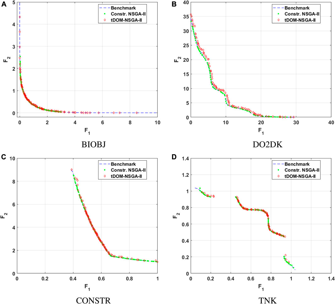
FIGURE 5. Pareto front of the biobjective problems generated via tDOM-NSGA-II.

Another observation that can be made based on the visual representation of the generated Pareto fronts, is that the solutions generated by the tDOM-NSGA-II algorithm for the DO2DK-problem would appear to have not fully converged to the benchmark Pareto front. This apparent loss in convergence is a consequence of the introduction of the trade-off of solutions as a stopping parameter. When the PIT-regions of the solutions making up the benchmark Pareto front are constructed, a so-called zone of insignificance is formed in the close proximity of the Pareto front (see Figure 6). Solutions located within this zone of insignificance are not considered to be significantly different to the benchmark solutions by the decision maker. Thus if the loss of convergence is limited to this to zone of insignificance, the solutions have sufficiently converged according to the decision maker. In Figure 7, the zone of insignificance for the DO2DK-problem is graphically displayed as well as the solutions generated with the tDOM-NSGA-II algorithm. From a visual analysis, it can be clearly seen that all solutions generated with the tDOM-NSGA-II algorithm have converged within the zone of insignificance.

FIGURE 6

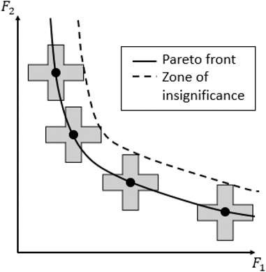
FIGURE 6. Zone of insignificance of a bi-objective optimisation problem.

FIGURE 7

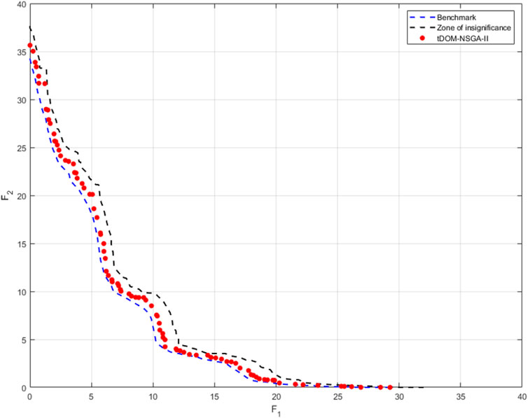
FIGURE 7. Graphical representation of the zone of insignificance of the DO2DK-problem.

If, however, the decision maker requires a closer approximation of the Pareto front, this can be obtained by decreasing the $\text{Δ}t$ and $\text{Δ}r$ values, defining the PIT-region. By doing so, the width of the zone of insignificance will also decrease, allowing solutions to converge more closely to the Pareto front, whilst reducing the trade-off-based resolution of the Pareto front (i.e., more insignificant solutions will be displayed).

Finally, considering the discontinuous Pareto front of the TNK-problem (seeFigure 5D), it can be seen that both algorithms have no difficulties with generating a discontinuous Pareto front. No solutions were generated in the discontinuous areas and the extremities of the continuous parts of the Pareto front are not problematic points. Additionally, all the generated solutions have converged to the benchmark TNK Pareto front.

To obtain a quantitative indication on the algorithm’s performance, the performance parameters FPOS, MID, and SNDS are calculated during every iteration of the algorithm. The optimisation process for each case study is repeated 10 times, to be able to statistically analyse both algorithms’ performances. The evolution of the performance parameters in function of the amount of iterations for the bi-objective numerical case studies is represented in Figure 8. Note that the iteration-axis was cropped for the sake of clarity. The final values of all the performance parameters are summarised in Table 2. The final FPOS-value is not reported in Table 2 as it always reached it’s maximum value of 1.00 for the constr. NSGA-II. On the other hand, the trade-off-based stopping criterion of the tDOM-NSGA-II algorithm requires that the FPOS of the solution population was equal to 1.00, otherwise the stopping criterion was not activated.

FIGURE 8

FIGURE 8. Comparing performance plots of the tDOM-NSGA-II algorithm and the constrained NSGA-II algorithm (average taken over 10 runs) for the BIOBJ-problem (A), the DO2DK-problem (B), the CONSTR-problem (C), and the TNK-problem (D). The iteration axis is cropped.

TABLE 2

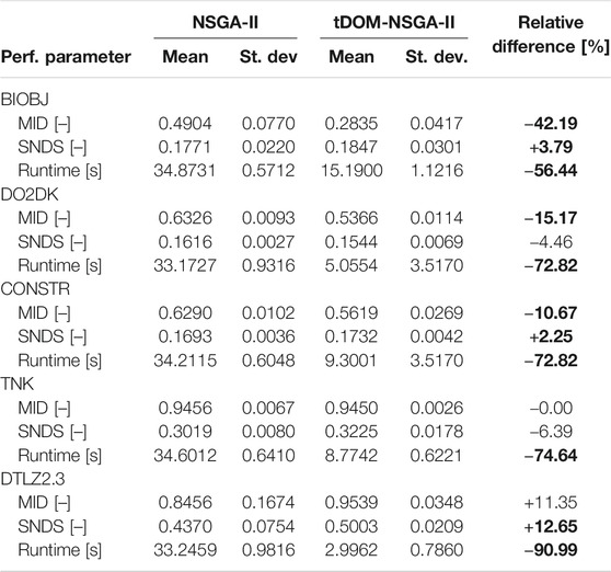
TABLE 2. Performance parameters and runtime of the bi- and three-objective case studies, generated with the constrained NSGA-II algorithm (Constr. NSGA-II) and the developed t-DOM-NSGA-II algorithm. Relative differences marked in bold indicate that the tDOM-NSGA-II algorithm outperformed the NSGA-II algorithm.

The fact that, in the case of the constr. NSGA-II algorithm, the FPOS performance parameter is always equal to 1.00, means that the final solution population always consisted out of non-dominated solutions. Moreover it was observed that the maximum number of iterations, i.e., 75, was set too high. The solution population already consisted entirely out of non-dominated solutions after only a fraction of the iterations. Continuing the constr. NSGA-II optimisation-process after the FPOS reached 1.00 meant that a lot of computation time was spent on unnecessary further iterations. Two valid arguments to continue the optimisation-process nonetheless, are on one side the anticipation that the solutions will further converge to the Pareto front, and on the other side the anticipation that solution diversity will increase.

The first argument however implies that eventually, whilst the iteration process continues, new non-dominated solutions are generated. Because these solutions are more closely located to the Pareto front, it can be expected that they will dominate one or more solutions of the non-dominated solutions of the previous iteration. Thus, if it were the case that the solutions would further converge to Pareto front, it is likely that the number of non-dominated solutions would fluctuate. This is however not the case. Once the solution population consists entirely out of non-dominated solutions, it stays this way until the maximum number of iterations is reached. On the performance plots in Figure 8 it can be seen that once the FPOS-value reaches its maximum value of 1.00, the standard deviation also decreases to 0.00, indicating that over the ten repetitions, the FPOS-value of the solution population did not fluctuate once it reached its maximum value.

Concerning the MID- and SNDS-values presented in Figure 8, the average MID-values of the BIOBJ- and CONSTR-problem increase after the FPOS has reached its maximum value and the iteration process continues. The average MID-values of the DO2DK- and TNK-problem on the other hand reach a constant value after FPOS has reached its maximum value and the algorithm is not stopped. An increase in MID means that the average Euclidean distance between the solutions and the Utopia point increases, i.e., the solutions move away from the Utopia point. This is obviously an unwanted scenario because this means that convergence of the solutions to the Pareto front diminishes if the algorithm is not stopped. Although an increase in MID can also indicate an increase in solution diversity, it is not considered to be the case in this scenario while the increased MID is accompanied with an SNDS that stabilises when the iteration process is continued. The observed stabilisation or decrease in convergence further renders the first argument to continue the iteration process after FPOS equals 1, i.e., the anticipated increased convergence, invalid.

The second argument to continue the iteration process after the FPOS has reached its maximum value, i.e., the anticipation that the solution diversity will increase, is also proven invalid based on Figure 8. An increase in solution diversity is indicated by an increase in the SNDS-value. However, it can be seen for all the bi-objective case studies that the SNDS-value stabilises. The continuation of the iteration process thus has no major influence on the solution diversity. This observations proves that the anticipated increase in solution diversity is no valid argument to continue the iteration process after FPOS equals 1.

Table 2 indicates a significant decrease in runtime for all the bi-objective case studies, ranging from 56.44% up to 84.76% faster on average. In terms of convergence, Table 2 signifies a decrease in MID for all the bi-objective case studies when the Pareto front is generated with the tDOM-NSGA-II algorithm. Based on the visual representation of the Pareto fronts in Figure 5 however, this is contradictory. As already mentioned, the Pareto front of the DO2DK-problem displays an apparent decreased convergence in comparison with the Pareto front generated with the constr. NSGA-II algorithm due to the presence of the zone of insignificance. The decrease in MID is in this scenario thus most likely not the result of an increased convergence. It is found that the normalisation step of the objective functions is the cause of the decreased MID. Because the anchor points are included in the solution population, the objective range at which solutions are generated becomes larger. The majority of solutions however is generated within the same range as it were the case with the constrained NSGA-II algorithm. Yet, these solutions are in case of the tDOM-NSGA-II algorithm relatively closer to the Pareto front than the constrained solutions because the anchor points now determine the objective range.

5.2 Three-Objective Case Study

The Pareto fronts and corresponding benchmark of the DTLZ2.3-problem are represented in Figure 9A. The corresponding performance plots are represented in Figure 9B. The values of the performance parameters after the iteration process is terminated are included in Table 2.

FIGURE 9

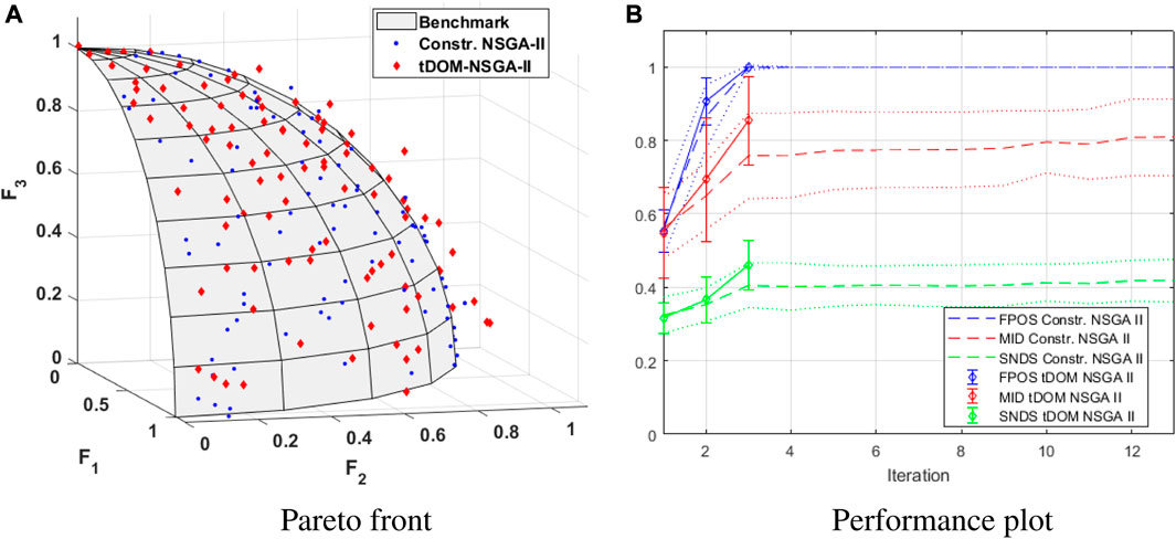
FIGURE 9. Pareto front (A) and performance plot (B) of the DTLZ2.3-problem, generated via tDOM-NSGA-II.

Figure 9B displays that the FPOS of the solution populations generated by the constr. NSGA-II algorithm quickly reaches its maximum value. The MID of the constr. NSGA-II algorithm keeps increasing, but this is accompanied with an increase in SNDS while FPOS <1. In case of the constr. NSGA-II algorithm, the early increase in MID is therefore most likely the result of the diversification of the solution population. However, once the FPOS reached its maximum value of 1.00 and the optimisation process was continued, the MID of the constr. NSGA-II algorithm continued to increase but the SNDS tended to stabilise. This increase in MID is no longer the result of the diversification of the solution population but a result of the diminishing convergence of the solutions. Based on these observations, it can again be concluded that the continuation of the optimisation process after FPOS = 1 is futile.

When considering the solutions generated with tDOM-NSGA-II, on first glance it would again seem that the solution convergence is less in comparison with the solutions generated with the constr. NSGA-II algorithm. Anew, this can be the consequence due the introduction of the trade-off as an additional selection parameter. Nonetheless, the convergence of the solutions for this case study, is unsatisfactory especially for low $F_3$ objective costs. The performance parameters are represented in Table 2. The most significant gain of the tDOM-NSGA-II over the constr. NSGA-II is the decrease in runtime of 90.99% on average.

5.3 Bi-objective Williams-Otto Reactor Case Study

The Pareto fronts generated by NSGA-II and tDOM-NSGA-II are displayed in Figure 10A. A first observation that can be made, is that the convergence of the tDOM-NSGA-II algorithm is not as good as that of the NSGA-II algorithm. As already mentioned, this apparent loss in convergence is due to the introduction of the trade-off-based solution selection (i.e., the zone of insignificance). Nonetheless, the tDOM-NSGA-II algorithm is capable of producing a qualitatively decent representation of the Pareto front. Note as well that the solution density in the low trade-off areas on the extremities of the Pareto front, is lower whereas the NSGA-II algorithm does not make this distinction. tDOM-NSGA-II needed, on average over 10 runs, 28 iterations, or a runtime of 413.1 s ± 110.3, while the NSGA-II algorithm completed all 75 iterations, requiring, on average, 1,086.0 s ± 27.6, resulting in a runtime reduction of 61.96% on average. The performance plots of the NSGA-II and tDOM-NSGA-II algorithms are represented in Figures 10B,Crespectively. Although the convergence of the tDOM-solutions is seemingly lower, based on Figure 10A, the average MID-value of the tDOM-NSGA-II algorithm is slightly lower than that of the NSGA-II algorithm, indicating a better convergence. This could be the result of the higher solution density in the knee, or central, area of the Pareto front. Solutions located in this area are nearer to the Utopia point than solutions located on the extremities of the Pareto front. The larger share of high trade-off solutions in the case of the tDOM-NSGA-II algorithm could have caused this lower MID-value, despite the lower overall convergence of tDOM-solutions.

FIGURE 10

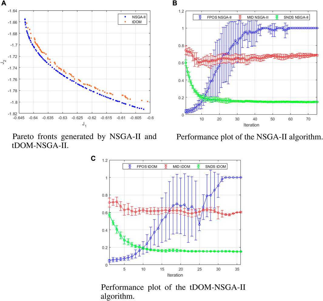
FIGURE 10. Pareto fronts of the Williams-Otto reactor case study generated by NSGA-II and tDOM-NSGA-II (A), and their respective performance plots (B) and (C).

Based on the bi-objective, three-objective, and Williams-Otto reactor case studies it can be concluded that the t-domination based stopping criterion results in an extensive reduction in runtime. Additionally the high trade-off solutions are emphasised by the tDOM-algorithm. The two major targets during the development of the tDOM-algorithm are thus fulfilled.

5.4 Overall Discussion

The two most significant and noticeable improvements of the tDOM-NSGA-II algorithm over the NSGA-II algorithm, are 1) the decreased number of iteration needed and the corresponding decrease in runtime, and 2) the trade-off-based solution resolution of the Pareto front.

The trade-off-based stopping criterion results in terminating the algorithm once all solutions in the current solution population are insignificantly different from those that made up the previous solution population from a trade-off point of view. Although introducing the trade-off function resulted in additional solution comparison and, thus, a more complex algorithm, it still performed better runtime-wise than its simpler counterpart, NSGA-II. This is due to the fact that the number of iterations that are ultimately needed during the optimisation process have a far greater influence than the number of comparison that are required during one single iteration. Note as well that the case studies presented in this contribution are computational inexpensive problems. While these optimisation algorithms will ultimately be employed for the optimisation of, i.a., complex (bio-)chemical processes, (logistic) network problems, etc., the generation of the solutions will become the most expensive step of the entire optimisation process. Generating solutions in these scenarios often involves computational expensive simulations, so it is essential in those scenarios that the overall amount of solutions that has to be generated in order to obtain a satisfactory Pareto front is kept to an absolute minimum. Reducing the amount of iterations required in order to obtain this Pareto front, will have the biggest influence on this. Even for the inexpensive numerical and dynamic case studies presented in this contribution, iteration reductions between 57.33 and 90.67%. The three-objective case study even displayed a 96.00% reduction in iterations required.

The introduction of this trade-off-based stopping criterion, however, resulted in an apparent loss in solution convergence due to the introduction of the so-called zone of insignificance. The reasoning behind the functionality of the trade-off-based stopping criterion also relies on an elitist approach built into the algorithm. This implies that the best solutions of the previous iteration are kept unchanged in the current one. This assures the user that, with progressing iterations, the solutions in the solution population are at least equally well converged and diverse as those of the previous iterations. If all solutions have converged sufficiently enough to the Pareto front, the difference between two subsequent solution generations will become smaller. The trade-off-based stopping criterion’s functionality is based on this principle and, in essence, is used to quantify how small this difference between two subsequent solution generations has to become in order to call it negligible and, as a result, stop the algorithm. It states that once all solutions of two subsequent solution generations are located within each others’ PIT-region, the difference between those two solution generations has become negligibly small for the decision maker. Improvement-based stopping criteria are already implemented in the context of single-objective evolutionary algorithms (Zielinski and Laur, 2008). The concept of t-domination allows for assessing the improvement evolution of solutions in a multi-dimensional objective space. The trade-off parameters can be seen as threshold values for improvement, just like the gradient based optimisation algorithms offer a termination criterion based on the threshold established for the first-order optimality. The comparison of solution generations is made as they evolve towards the Pareto front, as the benchmark Pareto front is unknown in real-life optimisation scenarios. Nonetheless, for the presented case studies, the benchmark Pareto front is known and the convergence of the generated solutions can be compared to it. The benchmark Pareto front inevitably consists of solutions itself, all of which possess a PIT-region. If the same reasoning is followed, the solutions on the Pareto front can be regarded as the utopian final solution generation. The algorithm will stop if the solution population that was obtained in the antecedent iteration was located entirely in the PIT-regions of the solutions located on the Pareto front. In other words, this antecedent solution population would have converged into the zone of insignificance which consists out of the PIT-regions of the solutions on the Pareto front. From the decision maker’s point of view, however, this antecedent solution population is equally good as the one that is fully located on the Pareto front as the decision maker does not consider the difference between the two to be significant. Therefore, as in real-life optimisation processes the Pareto front is unknown upfront, the goal is to converge until all solutions are located in the zone of insignificance.

The design of the tDOM-NSGA-II algorithm allows decision makers to quickly explore where the high trade-off regions are located for their proposed problem because of the trade-off-based stopping criterion and solution selection process, which was the second objective when developing the tDOM-NSGA-II algorithm. The trade-off-based solution selection step results in a less cluttered Pareto front, only displaying solutions of interest to the decision maker. The generated Pareto fronts of the presented cases studies with the tDOM-NSGA-II algorithm indeed display a trade-off-based resolution, with a high solution density in high trade-off Pareto front areas. If desired, these high trade-off areas can be further explored, potentially also with a view to increase the solution convergence to the Pareto front.

Regarding these observations, a next step could be to make the optimisation process more interactive. Bortz et al., (2014) already introduced the concept of interactive Pareto front navigation and exploration with the use of deterministic algorithms. The presented tDOM-NSGA-II algorithm is, as it is a swift but, potentially, cruder optimisation algorithm, perfectly suited to quickly generate highly informative Pareto fronts. Especially in the context of black-box optimisation problems, it would be a well-suited go-to algorithm for generating a cruder, but yet highly informative, Pareto front as the algorithm is additionally capable of including the decision makers’ preferences into the optimisation process. Based on the presented Pareto front, the decision makers could then be able to indicate which (high trade-off) Pareto front areas they want to explore in more detail by interacting accordingly with the algorithm. This process could additionally be coupled with a decision making support approach, guiding the decision makers’ through the decision making process. This would eventually result in highly customised Pareto fronts and optimal working points (i.e., the eventually selected solution(s)).

6 Conclusion

A sustainable process operation requires optimality with respect to multiple, often conflicting, objectives. A typical example of such conflicting objectives are economic, societal and environmental objectives. Such problems consisting of different conflicting objectives are called multi-objective optimisation problems (MOOPs). In such a case, not a single optimal solution exists, but multiple trade-off solutions exist. The set of these equally optimal trade-off solutions is called the Pareto set, from which a decision maker can select an operating point for implementation.

Different algorithms exist to solve MOOPs. The focus of this article has been on the evolutionary multi-objective optimisation algorithm NSGA-II. The basic philosophy of these algorithms is based on biological reproduction and evolution. Based on evolutionary principles, new solutions are created from parent solutions and by only selecting the best solutions for further reproduction, the generated solutions eventually converge to the most optimal solutions of the MOOP, or the Pareto front.

NSGA-II is widely acclaimed by researchers and users alike. Based on the results of five numerical benchmark case studies, two shortcomings were pointed out: 1) the algorithm lacks the ability to distinguish high trade-off solutions from low trade-off solutions and 2) the default stopping criterion proposed by Deb et al., (2002) based on reaching a user-defined maximum number of iterations, had no relevance to the concerned problem.

The tDOM-NSGA-II algorithm has been developed to overcome these shortcomings. This algorithm can distinguish between solutions based on their trade-off via the construction of regions of practically insignificant trade-off (PIT-regions). The more crowded the PIT-region of a solution is, the less favourable the trade-off of the solution is. The tDOM-algorithms stops if all the solutions of two subsequently generated solution populations are located within each other PIT-region. The tDOM-NSGA-II algorithm has been applied to five scalar benchmark case studies and one dynamic benchmark case study. The novel algorithm is capable of generating a Pareto front with a trade-off based solution resolution and displays a significant decrease in computation time required. This reduction in runtime ranges from 56.44% faster on average, up to 84.76% faster on average for the bi-objective case studies. For the three-objective case study, a runtime reduction of 90.99% on average was even obtained. The average runtime of the dynamic case study was reduced by 61.96%. The solutions generated by the tDOM-NSGA-II algorithm do display an apparent loss in convergence, due to the introduction of the zone of insignificance, which is made up out of the overlapping PIT-regions of solutions located on the Pareto front itself. Once solutions have converged into this zone of insignificance, defined by the $\text{Δ}t$ and $\text{Δ}r$ values provided by the decision maker, the decision maker does not consider the solutions of the population to be significantly different from those on the Pareto front.

Data Availability Statement

The original contributions presented in the study are included in the article/Supplementary Material, further inquiries can be directed to the corresponding author.

Author Contributions

Conceptualisation: VDB, PN, IH, CAML, and JVI; Investigation and literature review: VDB; Resources: VDB, PN, IH, CAML, and JVI; Writing, original draft preparation: VDB and PN; Writing, review and editing: VDB, PN, and JVI; Visualisation: VDB; supervision: JVI; Project administration: JVI; Funding acquisition: JVI. All authors contributed to the article and approved the submitted version.

Funding

This work was supported by the KU Leuven Research Council (OPTEC Center-of-Excellence Optimization in Engineering OPTEC and project C24/18/046), by the ERA-NET FACCE-SurPlus FLEXIBI Project, co-funded by VLAIO project HBC.2017.0176, by the Fund for Scientific Research-Flanders (projects G.0863.18 and G.0B41.21N), and by the European Union’s Horizon 2020 Research and Innovation Programme (Marie Sklodowska-Curie grant agreement numbers 813329 and 956126). VDB is supported by FWO-SB grant 1SC0920N. CAML holds VLAIO-Baekeland grant HBC.2017.0239. IH is supported by FWO-SB grant 1S54217N.

Conflict of Interest

The authors declare that the research was conducted in the absence of any commercial or financial relationships that could be construed as a potential conflict of interest.

References

Asefi, H., Jolai, F., Rabiee, M., and Tayebi Araghi, M. E. (2014). A hybrid nsga-ii and vns for solving a bi-objective no-wait flexible flowshop scheduling problem. Int. J. Adv. Manuf Technol. 75, 1017–1033. doi:10.1007/s00170-014-6177-9

CrossRef Full Text | Google Scholar

Back, T. (1996). Evolutionary algorithms in theory and practice: evolution strategies, evolutionary programming, genetic algorithms. New York, NY: Oxford University Press. doi:10.1108/k.1998.27.8.979.4

CrossRef Full Text

Bhaskar, V., Gupta, S. K., and Ray, A. K. (2000). Applications of multiobjective optimization in chemical engineering. Rev. Chem. Eng. 16, 1–54. doi:10.1515/revce.2000.16.1.1

CrossRef Full Text | Google Scholar

Bortz, M., Burger, J., Asprion, N., Blagov, S., Böttcher, R., Nowak, U., et al. (2014). Multi-criteria optimization in chemical process design and decision support by navigation on pareto sets. Comput. Chem. Eng. 60, 354–363. doi:10.1016/j.compchemeng.2013.09.015

CrossRef Full Text | Google Scholar

Branke, J., Deb, K., Dierolf, H., and Osswald, M. (2004). “Finding knees in multi-objective optimization,” in Parallel problem solving from nature - PPSN-VIII, Editor X. Yao (Berlin, Heidelberg: Springer) 722–731. doi:10.1007/978-3-540-30217-9_73

CrossRef Full Text | Google Scholar

Das, I., and Dennis, J. (1997). A closer look at drawbacks of minimizing weighted sums of objectives for pareto set generation in multi-criteria optimization problems. Struct. Optim. 14, 63–69. doi:10.1007/bf01197559

CrossRef Full Text | Google Scholar

Das, I., and Dennis, J. (1998). Normal-boundary intersection: a new method for generating the pareto surface in nonlinear multicriteria optimization problems. SIAM J. Optim. 8, 631–657. doi:10.1137/s1052623496307510

CrossRef Full Text | Google Scholar

Deb, K., and Goel, T. (2001). “Controlled elitist non-dominated sorting genetic algorithms for better convergence,” in Evolutionary multi-criterion optimization. Editors E. Zitzler, L. Thiele, K. Deb, C. A. Coello Coello, and D. Corne (Berlin, Heidelberg: Springer), 67–81. doi:10.1007/3-540-44719-9_5

CrossRef Full Text | Google Scholar

Deb, K., and Jain, H. (2014). An evolutionary many-objective optimization algorithm using reference-point-based nondominated sorting approach, part I: solving problems with box constraints. IEEE Trans. Evol. Computat. 18 (4), 577–601. doi:10.1109/tevc.2013.2281535

CrossRef Full Text | Google Scholar

Deb, K., Pratap, A., Agarwal, S., and Meyarivan, T. (2002). A fast and elitist multiobjective genetic algorithm: NSGA-II. IEEE Trans. Evol. Computat. 6 (2), 182–197. doi:10.1109/4235.996017

CrossRef Full Text | Google Scholar

Deb, K., Thiele, L., Laumanns, M., and Zitzler, E. (2005). Scalable test problems for evolutionary multiobjective optimization. London, UK: Springer, 105–145. doi:10.1007/1-84628-137-7_6

CrossRef Full Text

Ernst, P., Zimmermann, K., and Fieg, G. (2017). Multi-objective optimization-tool for the universal application in chemical process design. Chem. Eng. Technol. 40, 1867–1875. doi:10.1002/ceat.201600734

CrossRef Full Text | Google Scholar

Haimes, Y., Lasdon, L., and Wismer, D. (1971). On a bicriterion of the problems of integrated system identification and system optimization. IEEE Trans. Syst. Man, Cybern. SMC 1, 296–297. doi:10.1109/tsmc.1971.4308298

CrossRef Full Text | Google Scholar

Hannemann, R., and Marquardt, W. (2010). Continuous and discrete composite adjoints for the hessian of the Lagrangian in shooting algorithms for dynamic optimization. SIAM J. Sci. Comput. 31, 4675–4695. doi:10.1137/080714518

CrossRef Full Text | Google Scholar

Hashem, I., Telen, D., Nimmegeers, P., Logist, F., and Van Impe, J. (2017). A novel algorithm for fast representation of a pareto front with adaptive resolution: application to multi-objective optimisation of a chemical reactor. Comput. Chem. Eng. 106, 544–558. doi:10.1016/j.compchemeng.2017.06.020

CrossRef Full Text | Google Scholar

Jain, H., and Deb, K. (2014). An evolutionary many-objective optimization algorithm using reference-point based nondominated sorting approach, part II: handling constraints and extending to an adaptive approach. IEEE Trans. Evol. Computat. 18 (4), 602–622. doi:10.1109/tevc.2013.2281534

CrossRef Full Text | Google Scholar

Kalami Heris, S. (2015). NSGA-II in MATLAB. Yarpiz, 2015. Available at: https://yarpiz.com/56/ypea120-nsga2.

Knowles, J., and Corne, D. (1999). “The pareto archived evolution strategy: a new baseline algorithm for pareto multi-objective optimisation,” in Proceedings of the 1999 congress on evolutionary computation-CEC99, Washington, DC, 6–9 July 1999 (IEEE), 98–105. doi:10.1109/CEC.1999.78191

Google Scholar

Liagkouras, K., and Metaxiotis, K. (2017). Enhancing the performance of moeas: an experimental presentation of a new fitness guided mutation operator. J. Exp. Theor. Artif. Intell. 29 (1), 91–131. doi:10.1080/0952813x.2015.1132260

CrossRef Full Text | Google Scholar

Lin, L., and Gen, M. (2009). Auto-tuning strategy for evolutionary algorithms: balancing between exploration and exploitation. Soft Comput. 13 (2), 157–168. doi:10.1007/s00500-008-0303-2

CrossRef Full Text | Google Scholar

Liu, T., Gao, X., and Yuan, Q. (2017). An improved gradient-based nsga-ii algorithm by a new chaotic map model. Soft Comput. 21, 7235–7249. doi:10.1007/s00500-016-2268-x

CrossRef Full Text | Google Scholar

Logist, F., Houska, B., Diehl, M., and Van Impe, J. (2010). Fast pareto set generation for nonlinear optimal control problems with multiple objectives. Struct. Multidisc Optim 42, 591–603. doi:10.1007/s00158-010-0506-x

CrossRef Full Text | Google Scholar

Logist, F., Vallerio, M., Houska, B., Diehl, M., and Van Impe, J. (2012). Multi-objective optimal control of chemical processes using ACADO toolkit. Comput. Chem. Eng. 37, 191–199. doi:10.1016/j.compchemeng.2011.11.002

CrossRef Full Text | Google Scholar

Marler, R. T., and Arora, J. S. (2010). The weighted sum method for multi-objective optimization: new insights. Struct. Multidisc Optim 41, 853–862. doi:10.1007/s00158-009-0460-7

CrossRef Full Text | Google Scholar

Martí, L., García, J., Berlanga, A., and Molina, J. M. (2016). A stopping criterion for multi-objective optimization evolutionary algorithms. Inf. Sci. 367–368, 700–718. doi:10.1016/j.ins.2016.07.025

PubMed Abstract | CrossRef Full Text | Google Scholar

Mattson, C. A., Mullur, A. A., and Messac, A. (2004). Smart pareto filter: obtaining a minimal representation of multiobjective design space. Eng. Optim. 36 (6), 721–740. doi:10.1080/0305215042000274942

CrossRef Full Text | Google Scholar

Messac, A., Ismail-Yahaya, A., and Mattson, C. (2003). The normalized normal constraint method for generating the pareto frontier. Struct. Multidiscip. Optim. 25, 86–98. doi:10.1007/s00158-002-0276-1

CrossRef Full Text | Google Scholar

Muñoz López, C. A., Telen, D., Nimmegeers, P., Cabianca, L., Logist, F., and Van Impe, J. (2018). A process simulator interface for multiobjective optimization of chemical processes. Comput. Chem. Eng. 109, 119–137. doi:10.1016/j.compchemeng.2017.09.014

CrossRef Full Text | Google Scholar

Rabiee, M., Zandieh, M., and Ramezani, P. (2012). Bi-objective partial flexible job shop scheduling problem: NSGA-II, NRGA, MOGA and PAES approaches. Int. J. Prod. Res. 50 (24), 7327–7342. doi:10.1080/00207543.2011.648280

CrossRef Full Text | Google Scholar

Reyes-Sierra, M., and Coello, C. A. C. (2006). Multi-objective particle swarm optimizers: a survey of the state-of-the-art. Int. J. Comput. Intell. Res. 2, 287–308. doi:10.1145/1143997.1144012

CrossRef Full Text | Google Scholar

Suman, B., and Kumar, P. (2006). A survey of simulated annealing as a tool for single and multiobjective optimization. J. Oper. Res. Soc., 57, 1143–1160. doi:10.1057/palgrave.jors.2602068

CrossRef Full Text | Google Scholar

Tanaka, M., Watanabe, H., Furukawa, Y., and Tanino, T. (1995). “Ga-based decision support system for multi-criteria optimization” in 1995 IEEE international conference on systems, man and cybernetics. Intelligent systems for the 21st century 5, Vancouver, BC, 22–25 October 1995 (IEEE), 1556–1561. doi:10.1109/ICSMC.1995.537993

Google Scholar

J. Valadi, and P. Siarry (2014). Applications of metaheuristics in process engineering. Cham, Switzerland: Springer International Publishing Switzerland. doi:10.1007/978-3-319-06508-3

CrossRef Full Text

Vallerio, M., Vercammen, D., Van Impe, J., and Logist, F. (2015). Interactive NBI and (E)NNC methods for the progressive exploration of the criteria space in multi-objective optimization and optimal control. Comput. Chem. Eng. 82, 186–201. doi:10.1016/j.compchemeng.2015.07.004

CrossRef Full Text | Google Scholar

Williams, T. J., and Otto, R. E. (1960). A generalized chemical processing model for the investigation of computer control. Trans. AIEE, Part I: Comm. Electron. 79, 458–473. doi:10.1109/tce.1960.6367296

CrossRef Full Text | Google Scholar

Yu, G., Chai, T., and Luo, X. (2011). Multiobjective production planning optimization using hybrid evolutionary algorithms for mineral processing. IEEE Trans. Evol. Computat. 15, 487–514. doi:10.1109/tevc.2010.2073472

CrossRef Full Text | Google Scholar

Yuen, S., Lou, Y., and Zhang, X. (2018). Selecting evolutionary algorithms for black box design optimization problems. Soft Comput. 23, 6511–6531. doi:10.1007/s00500-018-3302-y

CrossRef Full Text | Google Scholar

Zielinski, K., and Laur, R. (2008). Stopping criteria for differential evolution in constrained single-objective optimization. Berlin, Heidelberg: Springer Berlin Heidelberg, 111–138. doi:10.1007/978-3-540-68830-34

CrossRef Full Text

Zitzler, E., and Thiele, L. (1999). Multiobjective evolutionary algorithms: a comparative case study and the strength pareto approach. IEEE Trans. Evol. Computat. 3 (4), 257–271. doi:10.1109/4235.797969

CrossRef Full Text | Google Scholar