 C. Brabant
 V. Dubreuil*
95% of researchers rate our articles as excellent or good
Learn more about the work of our research integrity team to safeguard the quality of each article we publish.
Find out more
ORIGINAL RESEARCH article
Front. Built Environ. , 05 September 2024
Sec. Urban Science
Volume 10 - 2024 | https://doi.org/10.3389/fbuil.2024.1455047
This article is part of the Research Topic Urban Morphology and Urban Thermal Environment View all 4 articles
The growth of a city is typically accompanied by densification and sprawl, the former through verticalization, urban renewal, and the filling in of empty spaces. All of these activities extend and intensify the urban heat island (UHI), which is quantified in this study as the difference in daily minimum temperature between urban and rural areas. Here, we investigate this phenomenon in the area of Rennes (France) and 17 surrounding cities using the Rennes Urban Network which comprises 93 weather stations. This study aims to 1) determine the optimal method for spatializing UHI in Rennes, France, 2) estimate and spatialize the UHI in the small peri-urban cities surrounding Rennes. For this, we model mean UHI and intense UHI using three methods of interpolation—multi-linear regression (MLR), ordinary kriging (OK), and regression kriging (RK)—based on data from 2022. We find that the RK method is the most suitable overall, with an RMSE of 0.11°C for mean UHI and 0.25°C for intense UHI. This approach allows stochasticity to be taken into account, and thus provides a better representation of UHI variation within Rennes and its peri-urban cities.
The urban heat island (UHI) effect is a climatic phenomenon caused by the expansion and verticalization of a city. It is expressed as the difference in near-surface air temperature between the city center and the surrounding rural areas (Oke, 1987) and has numerous impacts on the urban environment, including on human health, patterns of pollution (Rousseau, 2005; Stéphan et al., 2005; Ledrans, 2006), and vegetation growth (Mimet et al., 2009; Jochner and Menzel, 2015). Compared to the (semi)natural environment, the low vegetation density in cities, along with the high amount of artificial surfaces, lead to reduced evapotranspiration. The net radiation is stored in building materials, causing heat accumulation during the day and release at night, resulting in higher temperatures (Oke, 1976; Landsberg, 1981; Oke, 1982). Most efforts have focused on large sized cities (Cantat, 2004; Oswald et al., 2012; Shi et al., 2018; Rogers et al., 2019; Dos Santos, 2020; Cecilia et al., 2023) containing more than one million inhabitants according to the UN-Habitat report1 or medium-sized cities But, in 2014, almost one out of two people worldwide lived in a city with fewer than 500,000 inhabitants (Nations United, 2014), leading to an increasing recent works on mid-sized cities (Eliasson and Svensson, 2003; Schatz and Kucharik, 2014; Foissard, 2015; Wicki et al., 2018; Foissard et al., 2019; Amorim et al., 2021; Burger et al., 2021; Dumas, 2021; Richard et al., 2021; Marques, 2023Alonso and Renard, 2020; Oukawa et al., 2022; Voelkel and Shandas, 2017). Indeed, knowing and assessing the intensities of UHI observed in medium and small cities will enable to support public policies in new urban planning for more people. This study maps the UHI of the city of Rennes (medium size) and the surrounding peri-urban small cities, a region who have known an economic attractiveness which has led to intensive urbanization of the peri-urban cities in recent years.
UHI monitoring can be performed using data from fixed meteorological stations or transect measurements, or with thermal infrared data obtained by remote sensing (land surface temperature). Sometimes, a combination of several approaches is employed (Amorim et al., 2015; Wicki et al., 2018; Barbosa and Dubreuil, 2020). Land surface temperature data can be used to estimate surface urban heat islands (SUHI), which provide relevant and spatialized, but indirect, information on the atmospheric UHI. Currently, the only way to monitor atmospheric UHI over time is using measurements from meteorological stations of local air temperatures, but the spatial coverage of this approach is often restricted and may lack accuracy for interpolating continuous climatic phenomena, depending on the temporal and spatial scales of observation. To overcome these limitations, interpolation methods can be used to estimate urban temperatures from fixed data. These include so-called geostatistical methods, such as splines or inverse distance weighting, and so-called deterministic methods such as ordinary kriging (OK), multi-linear regression (MLR), geographically weighted regression (GWR), or regression kriging (RK) (Hengl et al., 2007; Harris et al., 2010; Zhang et al., 2011; Szymanowski and Kryza, 2012).
Previous studies of the UHI of Rennes have employed MLR to take into account a combination of land use variables and data from up to 28 weather stations (Dubreuil et al., 2008; Foissard, 2015; Foissard et al., 2019; Dubreuil et al., 2020). Although the geographical variables used have enabled good predictions of the UHI over the studied space, as a stochastic method, MLR develops errors due to the non-stationarity of the phenomenon because it does not take into account meteorological factors that can influence the distribution of the UHI (Foissard et al., 2019). To address this problem, other methods can be tested, such as OK, which takes account of the phenomenon’s non-stationarity, but requires a dense measurement network (Hengl et al., 2007). Hence, the network of weather stations has been densified, reaching about one hundred connected stations. They are currently used to monitor the air temperature (Dubreuil et al., 2022) in the study area, inside the ring road of Rennes but also in the nearby peri-urban cities. But using the OK method does not make it possible to maintain the relationship with land use as for MLR. Our proposal is to use hybrid methods such as RK which can also keep the phenomenon’s relationship with land use, while integrating the problem of non-stationarity.
The first objective of this study is to compare several interpolation methods (OK, MLR, and RK) and to determine which one is the most suitable for spatializing the UHI in a territory that is heterogeneous in terms of urban morphology, topography and variations in land use in rural areas. The second objective is to estimate and spatialize the UHI in the 18 small peri-urban cities surrounding Rennes. We considered only atmospheric UHI, derived from the air temperature near each station.
The study site encompasses Rennes and the surrounding suburban and peri-urban cities, which are located in Brittany, in western France, 43 km from the sea (Figure 1). The study area straddles a plateau in the northwest (105 m above sea level, asl) and a valley (20 m asl) in the south. Two major rivers cross the site, the one from the northeast to the south (“Ille”) and another from east to west (“Vilaine”), and converge in the city of Rennes.
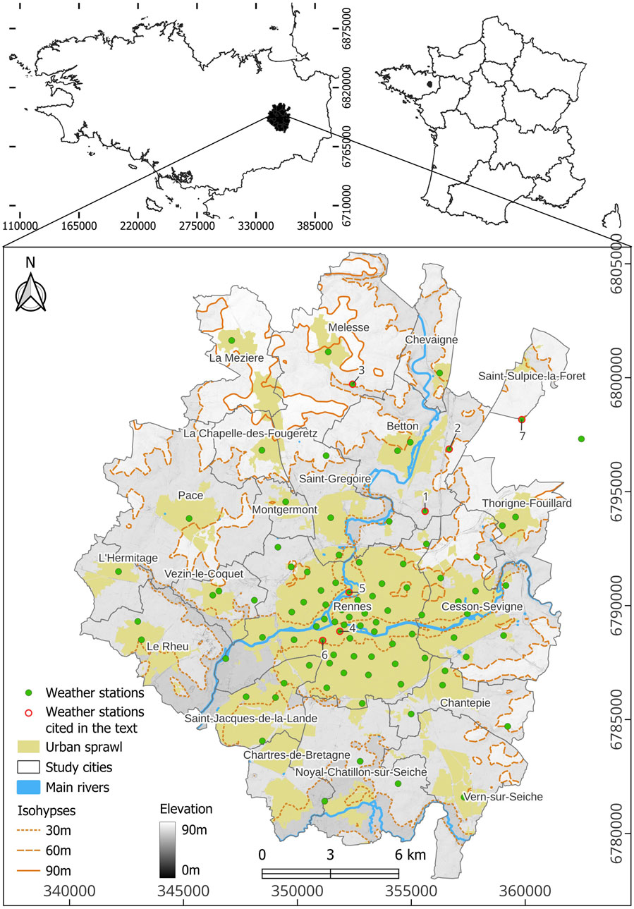
Figure 1. Urban sprawl of Rennes and peri-urban cities in 2020, with the location of weather stations indicated. Sources: AUDIARD and Corine Land Cover 2018. Datum: RGF93.
The temperate oceanic climate of Rennes is relatively cool and rainy, and is considered to be in class Cfb of the Köppen-Geiger classification (Eveno et al., 2016). The annual mean temperature is 12.4°C (1991–2020) with an average maximum daily temperature in July and August of 19.25°C and an average minimum of 6.22°C in January. The mean annual cumulative rainfall is 690 mm and the least rainy month is August, with 43.5 mm.
The population of Brittany has increased continuously since the middle of the 20th century. In 2019, this area had 3 323 355 residents (INSEE, www.insee.fr), and is predicted to face an increase of 12% by 2040 (400,000 more people, compared to 8% for mainland France). According to these scenarios, seniors (aged over 65) will represent 70% of the growth2. This population growth has been accompanied by a marked increase in urbanization (11.4% of Breton territory in 2016). Furthermore, the significant extension of artificial surfaces around major metropolises like Rennes (Figure 1) has enabled the development of a multitude of small and medium-sized towns. The conurbation of Rennes has experienced considerable urban sprawl over the last 30 years, with a 128% increase in artificial surfaces from 1985 to 2015 (SRADDET, 2019). Since the 2000s, Rennes has focused its efforts on slowing this sprawl and on densifying its existing impermeable surfaces and the population density of the city reaches 4500/km2 in 2020. This policy has had the effect of promoting the growth of peri-urban cities, making the Rennes region a model of an “archipelago city”. In total, the study area comprises 18 cities (Figure 1; Table 1), including Rennes and its smaller neighbors, which together host approximately 365,000 inhabitants in 352 km2. These small cities are representative of the interior of Brittany with respect to demographics, land pressure, and economics, and have grown rapidly in recent decades due to the influence of Rennes and the attraction of a “country” lifestyle. Specifically, this area features:
- One municipality of more than 200,000 inhabitants. Within Brittany, the five cities with more than 50,000 inhabitants (Rennes, Brest, Quimper, Lorient, and Vannes) represent 16% of the total population (INSEE).
- One municipality of approximately 17,000 inhabitants. Cities with a population between 10 and 20,000 inhabitants represent 12% of the population of Brittany.
- Eleven municipalities with a population between 5 and 15,000; cities of this size in Brittany represent 19% of the regional population.
- Five municipalities with a population between 2 and 5 000; cities of this size account for 27% of the population of Brittany.
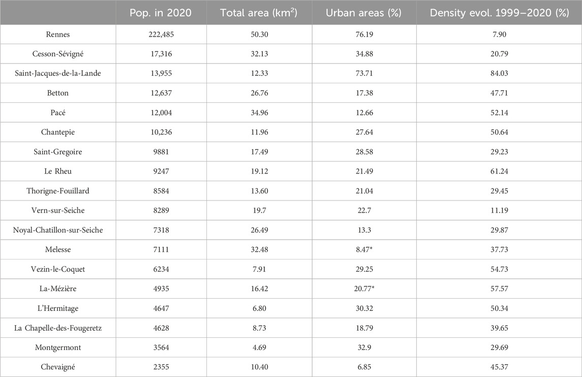
Table 1. Study cities and their overall population growth statistics. Sources: INSEE (2020 census), AUDIARD (data: “Urban sprawl” of Rennes metropolis from 2020), and *Corine Land Cover 2018 (Copernicus program, European space agency).
Historically, only the UHI of Rennes was studied from up to 28 weather stations. The network of weather stations has been densified inside the ring road of Rennes, reaching 51 connected stations. In addition, the nearby peri-urban cities have also been equipped to measure the intensity of UHI effects. In all, 127 connected stations are currently used to monitor the air temperature. The Rennes Urban Network consists of 32 Davis Vantage Pro2 (complete) weather stations connected by the internet and 95 Rising HF stations (Temperature and Humidity) connected by LoRaWAN, and is therefore available in real time3. Measurement sites are selected based on the local climate zones (LCZ), the choice of which is detailed in Dubreuil et al., 2022. The recording time step for Rising HF stations is 15 min. These temperatures are then averaged on an hourly basis.
To characterize the UHI, 93 Rising HF stations are used in this study; two are excluded from the analysis because more than 20% of their data are outliers or missing. The weather stations are only used to fill in missing temperature data from the 93 Rising HF stations (representing 6% of the dataset in 2022). Missing temperature are filled in using stations with similar thermal behavior. To do this, a Pearson correlation is first calculated between the stations. Second, a linear regression is performed on daily minimum temperatures between the station with missing data and the one with the highest correlation. Next, the prediction of missing data is obtained using the regression model.
The UHI is defined as a difference in air temperature between urban and rural areas, and its presence is determined by a variety of weather conditions (Oke, 1982; Cantat, 2004). The optimal conditions for the formation of a UHI are a combination of low average daily wind (≤5 m/s) and a clear sky. In Rennes, the UHI is nocturnal phenomenon (Foissard et al., 2019). The daily UHI is estimated as the difference between minimum temperature recorded by each station and the rural reference. This method incorporates the coolest hour of the night, corresponding to the body’s recovery phase after a hot day (Stéphan et al., 2005; Foissard, 2015). In order to estimate the intensity of a UHI, it is critical to first define a pair of urban-rural stations as references. Furthermore, with these reference stations, it is necessary to take into consideration the local effects inherent in their geographical situation (e.g., topographic hollow, exposure on a crest) (Dumas, 2021); their climatic situation, from the local scale to microscale (e.g., very localized rain, exposure to prevailing winds) (Morris et al., 2001); and/or their direct environment (e.g., large lake) (Mohsin and Gough, 2012). One solution is to use several stations as references, accounting for their direct environments and their location (north, east, south, west) relative to the urbanized spaces (Santamouris, 2015). This is especially important when a study focuses on a city at the bottom of a valley with an accentuated topography (Dumas, 2021). Here, we select the 3 rural stations (“La-Lice,” “La-Morinais,” “Melesse” respectively station 1, 2, 3 on Figure 1) with similar thermal behavior and identified as the coolest in the study area.
Next, we identified days in which a UHI is present, taking into account the connections between this phenomenon, land-use, and synoptic weather conditions. More precisely, the first step is to select all the absolute minimum temperatures that occurred at night (between 8 p.m. and 8 a.m.). We identified 191 days in which weather conditions are optimal for the formation of a UHI (wind speed ≤5 m/s and cumulative precipitation = 0 mm). Then, based on the recommendations of Garcia (1996), we filtered these results to retain only nights in which the UHI is at least of medium magnitude (≥2°C difference between the city center and rural reference). This yielded a total of 138 nights in 2022.
The purpose of interpolation techniques is to estimate unknown values in all points of the study area. This becomes complicated when, as is the case here, the phenomenon studied varies in space. This spatial variation can be separated into two components: the trend (first-order variation) and the spatial dependence (second-order variation) (Zhang et al., 2011). The trend can be modeled by spatial regression using georeferenced data with secondary characteristics, in our case, land use, urban morphology, or altitude. These data must be co-located with the data to be interpolated (here, UHI effects from temperature measurements). Instead, the spatial dependence can be characterized using a covariance function that estimates a semi-variogram, as proposed by kriging methods. The entire methodology is summarized in Figure 2 and described in more detail below. We first present MLR method and then kriging methods, including the one applied on MLR residuals.
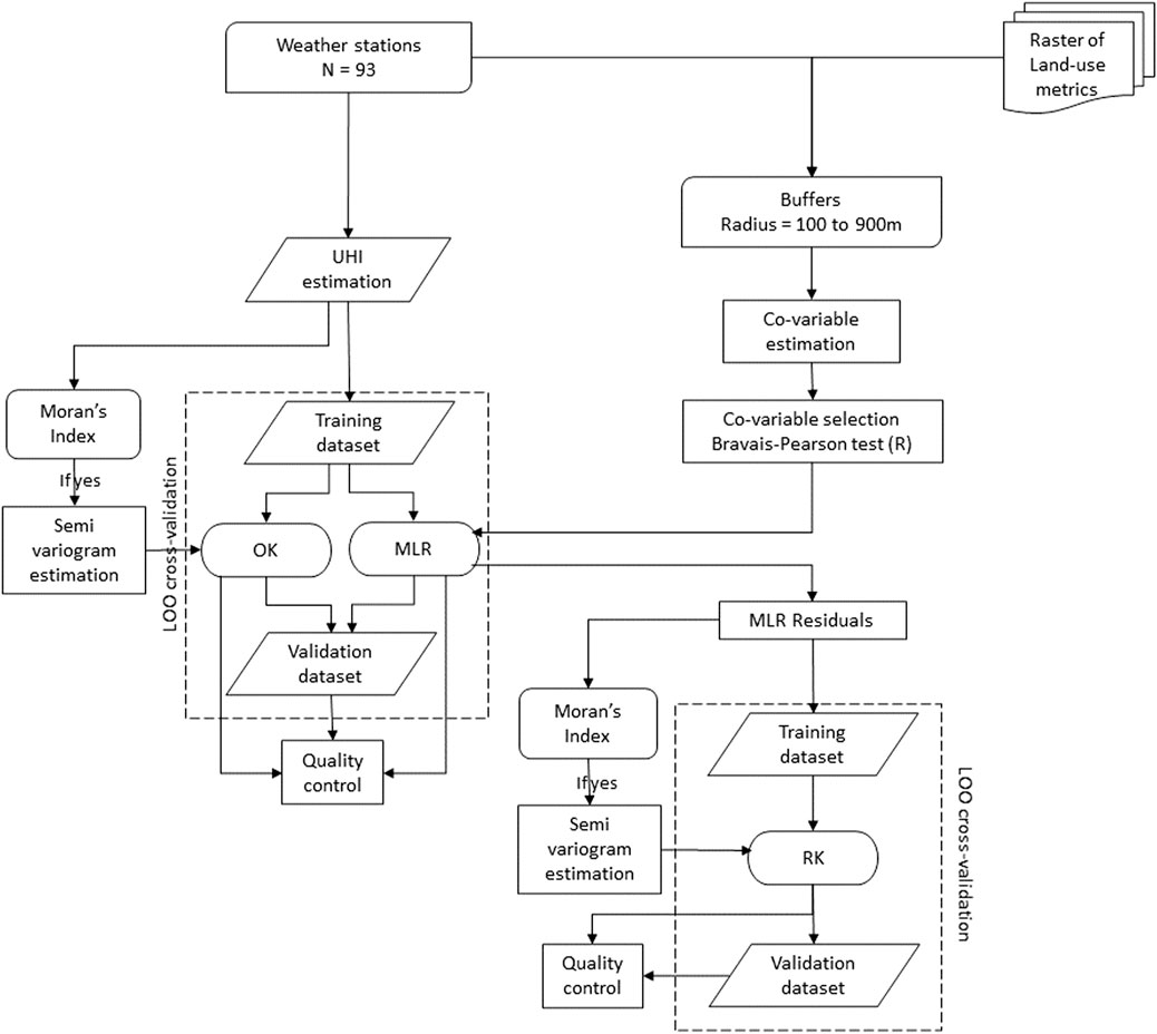
Figure 2. Flowchart of the applied methodology.
MLR, also called multi-criteria spatial regression, is considered an approximate global interpolation method. It provides the estimate and its associated error based on a statistical model, which can be expressed by Equation 1:
where
This method utilizes land use information as potential co-variables, which must be obtained from dense, accurate, and homogenous data networks. Here, we obtained these data from the National Institute of Geographic and Forest Information (IGN), which supplies geographical data (every year, here for 2021) under a free license (Etalab 2.0). IGN provides a variety of information on the ground surface, including the height of buildings, the road network, water surfaces, cultivated areas, and altitude. For information on vegetation in public and private areas, we obtained a GIS classification layer characterizing the fine-scale vegetation of the area from the services of “Rennes Métropole” (for 2017).
Using these data, we obtained the following metrics as potential co-variables (Table 2): built-up cover, height of buildings, impervious surfaces, high and low vegetation cover, water surfaces, distance to the center of Rennes (i.e., the distance to the “Boul-Liberté” station -station 4 on Figure 1- with the most intense UHI in Rennes), distance to the center of each city (distance to the city center station) and altitude. In addition, the sky view factor (SVF) is calculated based on altitude and the morphology of buildings (height and surface area); this gives an indication of building density and street geometry. SVF measures the diffuse radiation emitted by the surrounding surfaces: a low SVF is associated with increased net heat storage in buildings and therefore an increased UHI. The final resolution of all metrics is 3 m.
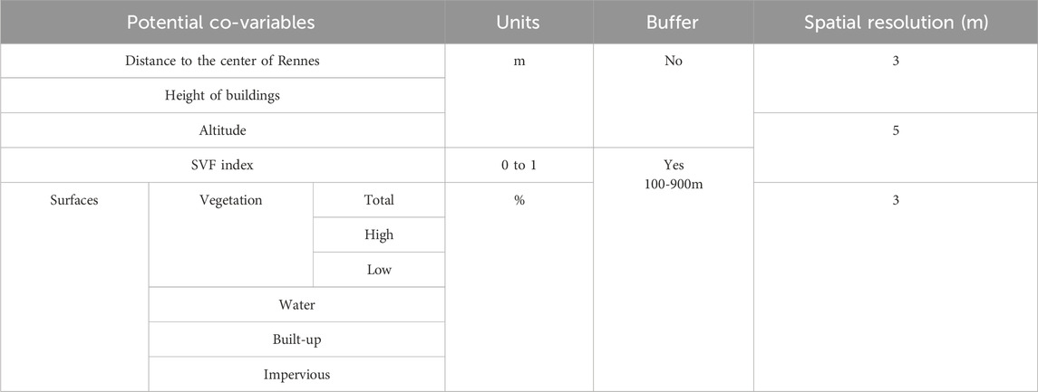
Table 2. Summary of co-variates and their characteristics.
As the land use surrounding the stations has a fluctuating influence on temperature in both time and space (Voogt and Oke, 2003; Amorim et al., 2015; Foissard, 2015), all metrics are re-calculated using multiple buffer sizes around the stations. Different radius sizes are tested, from 100 to 900 m with a step of 100 m, to determine the global influence of each metric, and the combination of metric and buffer size is subsequently called a co-variable. A detailed description of the method is given in the Supplementary material. This method is often used to determine the influence of a surrounding area on the UHI. For example, the influence of buildings on atmospheric temperatures is usually defined using a circle with a radius of 500 m (Eliasson and Svensson, 2003; Stewart and Oke, 2010; Zhao et al., 2011).
Finally, a linear regression model is built following the procedure explained by Foissard et al., 2019. First, the co-variables with the highest explanatory power are selected (Bravais-Pearson test - R); the total number of co-variables is limited to three in order keep the model as parsimonious as possible. Collinearity is also tested from the Variance Impact Factor and remains below 3 (maximum value = 2.17). Then, the best model is applied to the selected rasterized co-variables.
When data on land use are not available or sufficiently descriptive, or when the city is the finest scale of observation possible, geostatistical methods can be used. Many methods exist with various characteristics: stochastic or deterministic, local or global, and exact or inexact.
The most commonly used method is krige (krige, 1951; Matheron, 1967), which brings together a set of different geostatistical interpolation techniques. This approach measures the strength of statistical correlation as a function of distance, i.e., it quantifies the principle that objects closer to each other tend to be more similar than those farther away. Kriging assumes that the distance or direction between sample points reflects a spatial correlation that can explain variation in the parameter under study, and therefore its spatial structure distribution (at a regionalized scale). Kriging is considered an optimal and unbiased linear estimation method that uses the structural properties of the semi-variogram. In this study, if a variable is considered to be stationary but of unknown mean, ordinary kriging (OK) is used (Equation 2). The OK estimate is a linear weighted average of n observations defined as:
where
where Ε is the mathematical expectation in Equation 3 (detailed information available in Lloyd, 2005). Parameters and functions are optimized using the gstat and automap packages of R software.
The two methods explained above (MLR and kriging) can be combined to improve the results of the linear regression. Regression kriging (RK) takes into account both the trend and the spatial dependence. Regression (Equation 4) is used to fit the explanatory variables (the trend component, the deterministic part), and simple kriging (SK) with an expected value of 0 (the variable is stationary and of known mean) is then performed to fit the residuals of the linear model (the unexplained variation, the stochastic part), as follows:
where RKUHIi is the UHI effect calculated with SK on residuals for grid i, yi is the UHI effect calculated from regression, and εi is the regression residual interpolated with the SK approach. The predicted SK value εi for location i calculated as follow in Equation 5:
Where
The mathematical process is similar to universal kriging or kriging with external drift (KED), but the advantage of RK is the ability to extend it to a range of other regression techniques (Li and Heap, 2014). In addition, it is possible to interpret the two components of the interpolation method separately. This approach has been employed in many fields, for example, to examine soil properties (Odeh et al., 1995; Hengl et al., 2004; Zhu and Lin, 2010), remote sensing (Hengl et al., 2007; Kilibarda et al., 2014), climate (Bostan et al., 2012), and urban climate (Szymanowski and Kryza, 2009; 2012; Schatz and Kucharik, 2014; Touati et al., 2020; Colaninno and Morello, 2022; Ding et al., 2023).
The performance of each interpolation procedure is evaluated and compared for both of the UHI variables considered (see below) using cross-validation. Due to variability in land use across the study area (urban versus rural), the leave-one-out method (LOOCV) is chosen for cross-validation in order to analyze the optimal performance of each interpolation method. LOOCV uses a dataset of k = n-1 observations to calibrate the model on the training set, and n iterations of k = 1 for the validation set. The mean predictions from the validation dataset are compared to the observed data for each of the 93 test datasets. The quality and performance of interpolation are then evaluated based on the R2 value (or R2aj for multiple co-variables) as an indicator of the overall quality of the model and the RMSE as an indicator of the quantity of errors made by the model.
Given the RMSE’s sensitivity to outliers and the heterogeneity of the territory, spatial autocorrelation is assessed using the global Moran’s index and the tendency for clustering is evaluated with the local Moran’s index. Spatial autocorrelation is an extension of the principle of correlation between 2 variables, but takes into account the spatial location of the variable. The global Moran’s index is used to account for spatial correlation over an entire region. Its calculation is based on a weighted matrix which depicts the relationship between observations and their surroundings and measures their similarities between them as the product of their differences (Huo et al., 2012). Moran’s index provides insights into the predictive capacity of the model and helps to identify the spatial pattern of the UHI and any spatial outliers (Anselin, 1995; Szymanowski and Kryza, 2012; Lu et al., 2014; Colaninno and Morello, 2022). This index is calculated for both UHI variables (Section 2.4) and their residuals after MLR and before RK.
The mean absolute error (MAE) is also calculated as an indication of the overall quantity of errors from the model. Finally, the residual values obtained by the cross-validation process, extreme values, and their frequencies are studied in order to understand the model’s tendency to over- or under-estimate the UHI effect.
In this study, the interpolation methods described above are carried out using two estimates of UHI: the mean daily UHI in 2022, which took into account all 138 nights in which a UHI is present, and the mean of intense UHI in 2022, which is based on the 21 nights in which the UHI effect is ≥5°C (representing 6% of nights in 2022). The threshold of 5°C is chosen as a compromise—Garcia (1996) used 4°C as the definition of intense UHIs, but this yielded a much larger number of nights in Rennes in 2022 (18%), and ran the risk of smoothing out the local effects that we are trying to represent. Conversely, a threshold of 6°C produced a much smaller number of nights (only 6), which risked producing exacerbated microscale effects.
To reliably represent the local scale in an urban context and take the smallest buffer size into account (i.e., local variability), the spatial resolution of the final grid is 100*100 m over 352 km2. The parameters resulting from the analyses are then applied to each cell in order to reconstitute a continuous field of the UHIs across the territory.
From a climatic point of view, 2022 was an exceptional year all over the world. In Rennes and its peri-urban cities, temperatures were above normal (1991–2020), with a mean temperature of 13.6°C (normal = 12.4°C) and a new heat record of 40.5°C, reached on July 18. Typically, precipitation is distributed throughout the year (cumulative annual average = 690 mm), but 2022 saw marked periods of drought: in March, only half of the normal amount of precipitation fell (25 mm) and in July it rained only 1 mm (normal = 44 mm). Over the entire year, the cumulative rainfall total was 578.6 mm. In addition, a new record was set for the amount of sunshine (more than 2088 h, with 1762 h as the historical average), and 73 days experienced maximum temperatures of at least 25°C (normal = 43.5 days). There were therefore numerous, long, and intense heat waves that first started at the end of March and finished at the end of October. Although the temperate oceanic climate is generally too variable to be favorable to the development of intense UHIs, the year 2022 was hot, dry, and sunny. Overall, 52% of nights in 2022 were favorable—clear sky and low wind (<5 m/s) —for the development of UHIs.
As a first step in comparing UHI data from 2022 with those from 16 previous years (published in Dubreuil et al., 2020), we calculated the annual mean difference between station 5 and station 3. In 2022, this was 2.7°C, which corresponds to the previous record (2.7°C in 2019). Such deviations do not necessarily result from UHI conditions—synoptic weather conditions may play a role—but may be relevant to long-term monitoring efforts regarding UHIs and climate change. The high mean can be partly explained by the number of days in which the UHI effect was over 4°C, which was around one night out of four; however, this frequency was not higher than that of 2011. What appeared to have made the difference was the number of nights with a UHI intensity ≥6°C, which represented 3.29% of occurrences in 2022 compared with a historical average of 1.4%. Moreover, new UHI records were set on the night of July 17–18, when there was a simultaneous maximum difference of 9.5°C between station 5 and station 3 and 8.25°C between the Rennes center and rural reference (the previous record was 8°C in 2011-Figure 3).
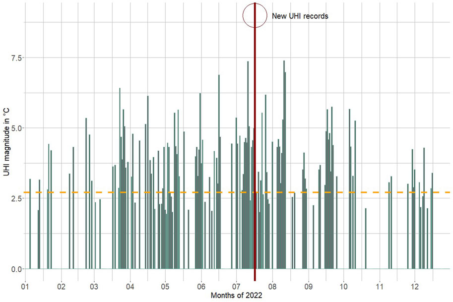
Figure 3. Distribution of UHI days in 2022. The conditions represented are: UHI ≥2°C, precipitation = 0 mm, and wind ≤5 m/s. Dashed yellow line: average UHI in 2022.
The first step in implementing MLR is selecting the most significant covariables to be used as the linear regression coefficients. To keep the results of the linear regressions comparable between mean UHI and intense UHI, the same co-variables are chosen in both cases. Both mean UHI and intense UHI are found to be highly correlated with SVF and the amount of impervious surfaces within a 600-m radius (R = −0.76 and 0.75) and a low amount of vegetation within a 100-m radius (R = −0.72). In the automated process, these metrics are selected most often for the models with relatively similar buffer sizes (at least on the same orders of magnitude). All three metrics are representative of the urban environment, since they reflect the extent of artificial surfaces and vegetation in a city along with its morphology and organization.
Based on analysis of the LOOCV error, RK is the most accurate method for spatial interpolation of both types of UHI (Table 3; Figures 4C,F), with an R2 = 0.98. For mean UHI, the RMSE is low, with only 0.15°C difference and residuals ranging from −0.60°C to 0.49°C. This degree of variability (under ±0.5°C) for residuals is considered low because this is within the range of measurement accuracy of the weather stations. Thus, RK demonstrated good predictive ability, with just one value over-estimated. For intense UHI, the RMSE remained low (0.25°C), with three extreme values, and the MAE remained very low, indicating the good predictive ability of the model. The variance explained by MLR under LOOCV is 78% for mean UHI and 75% for intense UHI (Table 3; Figures 4B,E). Despite this, the spatial variability of the phenomenon is only partially represented, as evidenced by the residuals which represented 30% of the dataset for mean UHI and 53% for intense UHI.
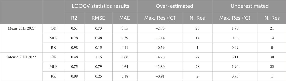
Table 3. Comparison of results between MLR, RK, and OK methods.
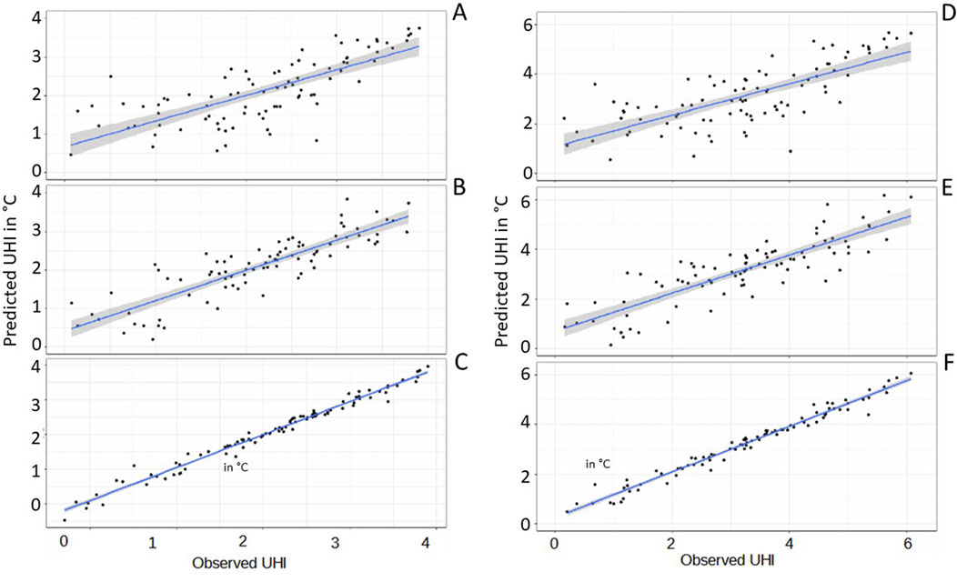
Figure 4. Scatterplots of observed versus predicted UHI according to LOOCV. On the left: mean UHI, on the right: intense UHI. (A) and (D) OK method, (B) and (E) MLR, (C) and (F) RK method.
The least accurate results are obtained with the OK method (Table 3; Figures 4A, 5D), which explained only about 50% of the variance. The conditions in this study are not optimal for OK since the spatial autocorrelation of both types of UHI is not uniform over the entire territory (Figures 6D, 7D). This invariably leads to prediction errors. Indeed, it has been stipulated that sampling points must be equally distributed over a territory in order to obtain satisfactory kriging (Hengl et al., 2007).
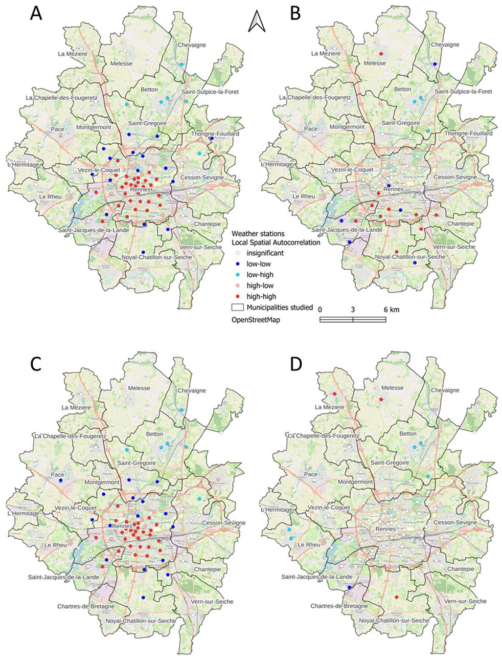
Figure 5. Statistically significant clustering tendency of Local Moran’s I for both types of UHI, (A) mean UHI, (B) MLR residuals; (C) intense UHI, (D) MLR residuals.
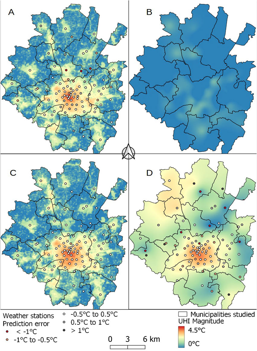
Figure 6. Interpolation of mean UHI. (A) MLR, (B) kriging on residuals of the MLR, (C) RK, (D) OK.
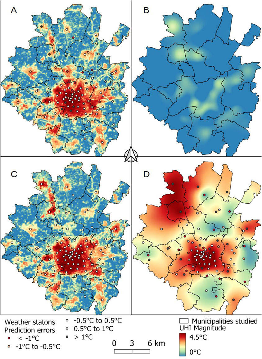
Figure 7. Interpolation of intense UHI. (A) MLR, (B) kriging on residuals of the MLR, (C) RK, (D) OK.
As expected, values of global Moran’s I are relatively strong for both mean UHI and intense UHI (Table 4). However, this analysis indicated that spatial autocorrelation is not uniform over the entire territory (close to 0). Rennes forms a hot spot, defined as High-High (Figure 5), while the vegetation belt around Rennes constitutes a cold spot (Low-Low) based on local Moran statistics. For the MLR residuals of both types of UHI, the global Moran’s I statistic reveals spatial autocorrelation (p-value <0.05), an essential condition for the use of RK. Furthermore, values of the Z-score of Moran’s I (Table 4) indicated that the spatial relationships are not uniform across the entire territory, supporting the existence of local dependencies or heterogeneity in residuals (High-Low or Low-High). In other words, the MLR performed well when predicting at a global scale (Moran’s I near 0) but is less accurate at the local scale, with some residual aggregations. This is expected due to the non-stationarity of the phenomenon arising from variability in land use within the territory (Anselin, 1995; Szymanowski and Kryza, 2012). One of the advantages of RK is that it is able to take into consideration the local trend within the search window (distance of the semi-variogram) by kriging non-stationary data (Li and Heap, 2014).
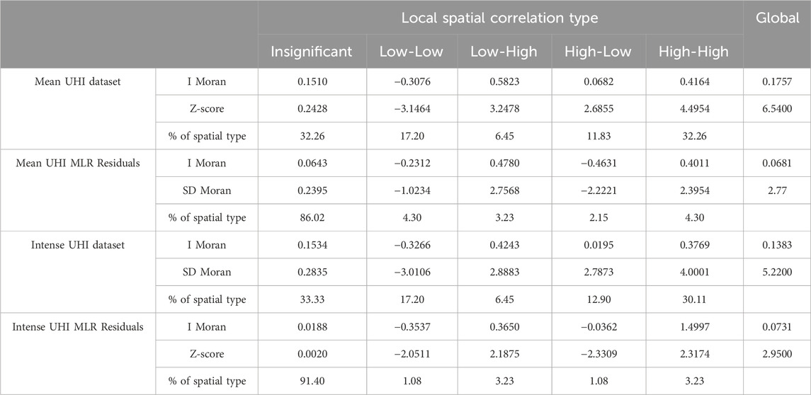
Table 4. Values of Moran’s I statistic, with Z-score, and local Moran’s I. p-value <0.05 for each test.
It is challenging to find a method that can estimate the spatial distribution of a UHI over a heterogeneous territory. The differences between the conurbation of Rennes, Cesson-Sévigné, and St-Grégoire and the small, peri-urban cities in the study area can cause difficulties with estimation, especially for the OK method. Moreover, the sampling pattern is irregular throughout the territory, which leads to the misestimation of peri-urban cities, non-representation of urban parks, and overestimation of rural areas.
MLR is able to estimate the mean UHI of the peri-urban cities and in Rennes (Figures 6A, 7A), with a clear gradient from the city center to the periphery. The historic center of the city of Rennes is a dense mix of midrise or low-rise buildings, with little vegetation (LCZ 2). The further one moves away from the city center, the more the city opens up into a tangle of individual and collective residential districts (LCZ 6 and 9). This gradient is not uniform, since the activity zones form certain hot spots that differed from urban or suburban areas (ZA-West, ZA North, ZA-South-East around Rennes, LCZ 8). In addition, these areas are also present in peri-urban cities such as Groupe PSA, Bourdonnais, and La Rigoudière. These highly artificialized and/or low-vegetation areas are characterized by differences of more than 2°C compared to the countryside. However, certain areas, such as the town of St-Grégoire and the rural area to the east, are overestimated by more than 1°C. Likewise, the “Prairies St. Martin” site, an urban park located in the northern part of the city of Rennes (station 5 on Figure 1) is also overestimated, with residuals of −0.89°C (mean UHI) and −1.18°C (intense UHI). This site has always presented difficulties for spatialization by MLR studies (Foissard, 2015; Foissard et al., 2019). Nevertheless, it has positive values of local Moran’s I (Low-Low) for both UHI types, while adjacent sites are characterized as High-Low. This is evidence of the cooling effect of this urban park at this spatial scale.
To the north of the study area, the cities of La-Mézière and Chapelle-des-Fougeretz have problems of underestimation. In that area, the spatial autocorrelation of MLR residuals revealed clusters in La-Mézière and Melesse (High-High), but only for intense UHI (Figure 5). Compared to other cities of comparable size (Table 1), these cities experience more-pronounced intense UHIs as a result of their topographic situation: they are located on a ridge at the base of higher ground (90 m versus 60 m - Figure 1), but higher than the Rennes valley (30 m), and thus do not benefit as much from the cold air that flows down into the valley and cools the countryside. Moreover, the land use in this area is largely dedicated to industrial zones and other activities known to store radiation during the day and release it at night in the form of heat. The southern districts of Rennes are also underestimated for both types of UHI. In this case, the underestimation may be due to larger spatial effects that could not be taken into account by the MLR, such as the influence of the synoptic winds. Indeed, it appears likely that the night wind has a structuring effect on UHI patterns: when the wind speed (>2 m/s) and direction (north/northeast/northwest) are favorable, the warm air moves from the city center towards the southern districts (Brabant et al., 2022).
Concerning intense UHI, MLR is able to estimate the phenomenon over the whole territory, but the errors are coarser and more heterogeneous than for the mean UHI. Patterns of over- and underestimation are the same as observed for the mean UHI.
The OK method is based on the principle of nearest-neighbor resemblance; if the sampling points do not represent a feature space with sufficient precision, then the spatial prediction will be poor (Hengl et al., 2007) and it will not be possible to correctly estimate the UHI. We find that this is particularly true when the phenomenon is intense and more heterogeneous in space (Figure 7D), because the spatial variability in the UHI represents a finer scale than can be captured by the distance between the measurement points.
With the RK method, the incorporation of stochasticity in the process of spatialization improved the results from both the quantitative and visual points of view (Figures 6C, 7C; Table 3). Similar errors that tended to cause clustering are eliminated, along with nearly all over- or underestimated areas. Indeed, the UHIs of the southern districts of the city of Rennes are more intense than those observed with the MLR, while the cooling effects of green spaces and peri-urban towns are better defined. Only one residual persisted for mean UHI (Station 5 on Figure 1: “Prairies Saint-Martin”; −0.59°C) and three for intense UHI: “Postuminus” (station 6) is underestimated by 0.95°C, while “Saint-Denis” (station 7) and “Prairies Saint-Martin” are overestimated by −0.54°C and −0.91°C, respectively.
Our first objective was to test several interpolation methods and determine which is best able to estimate UHI effects. In this study, we investigated several methods for predicting UHI based on data from a dense network of weather stations. We found that the most satisfactory method is the hybrid approach that combined multiple linear regression with kriging carried out on the residuals (RK). Our results demonstrated that regression kriging performed better in predicting spatial UHI patterns in and around Rennes than the previous method used in this area (MLR). Indeed, the use of RK better highlights extreme values that spatially form hotspots on the map. This makes it easier to identify areas where action to mitigate UHI is a priority.
The superior performance of RK has been demonstrated in numerous studies, but only a few have employed this method to analyze urban temperature (Colaninno and Morello, 2022; Ding et al., 2023; Touati et al., 2020) or UHI phenomena (Szymanowski and Kryza, 2009; Szymanowski and Kryza, 2012; Schatz and Kucharik, 2014). The drawback of this approach is that it requires a thorough knowledge of the kriging process, as well as high-quality input data in terms of number, geolocation, density, accuracy, and the spatial scale of representation, as described in Hengl et al., 2007.
The power of RK lies in the fact that it summarizes both the trend component (the deterministic part, explained by MLR) and the spatial dependence (the remaining stochasticity). RK then makes it possible to follow the spatial progression of a UHI (intensification or reduction) based on changes in land use. However, regression assumes the stationarity of the phenomenon, in other words, that the predictor seen as a stimulus yields the same response over the entire territory. For UHIs, this is not entirely true, as the local climate is necessarily influenced by other spatial processes (e.g., wind). In this study, the UHI is measured at numerous points, whose characteristics are related to the city’s complexity and morphology. Auxiliary data are also of good quality (IGN) and fine resolution, representing the fineness of the urban spaces (down town, rural and surrounding small cities, see 4.2). The question of the density of the network is also challenging: Ding et al. (2023) show that the number of stations in the center of Guangzhou can be reduced by 75% and that RK results remain similar. But for Foissard et al. (2019) were not able to use RK with only one-third of the stations we used for this study. As we added a greater area with new urbanization contexts it is not obvious to be able to reduce significantly the network density.
Szymanowski and Kryza, (2012); Schatz and Kucharik, (2014); Colaninno and Morello, (2022) tend to favor the use of local regression, and in particular, geographically weighted regression (GWR) (Fotheringham et al., 2003) in order to observe local variations in UHI. GWR produces MLR for every point in space using a subset of information from nearby points, and can therefore take into account the non-stationarity of the phenomenon. In particular, Szymanowski and Kryza (2012) demonstrated the utility of GWR for modeling UHI in the presence of significant winds using regular mobile measurements. Even in that case, though, GWR did not fully recognize the role of wind in shaping the UHI effect. Similar to the present work, those authors also showed that an analysis of residual stochasticity considerably improved the results both for MLR (RK) and GWR (GWRK). This provides a complementary perspective to the current study, and suggests that GWR or GWRK might be also relevant for estimating UHI in small and medium-sized cities.
Furthermore, this study did not take into account the temporal resolution of UHIs, only their intensity and annual averages. In studies that have focused on modeling at high temporal resolutions (infra-daily, hourly, day/night), the RK method has generally not been the most suitable approach (Szymanowski and Kryza, 2012; Schatz and Kucharik, 2014; Colaninno and Morello, 2022). One of the limitations of regression and kriging is that they are global methods. This means that they provide good results within a climatologically coherent area. When interpolation is applied to larger, more heterogeneous areas, the results are of lesser quality (Joly et al., 2008). This is because interpolation can be disrupted by the effects of opposing constraints, as is the case, for example, with accentuated relief (opposition between plains and mountains). The same is true at a more local spatial scale, where space is dependent on possibly different UHI formation systems for the same observation time window. In other words, the processes responsible for spatial variations in UHI do not operate in exactly the same way every time depending on meteorological situations.
Our second objective was to estimate the UHI effect in new territory (small cities) and to find an effective method for representing it as faithfully as possible in cities of different sizes. As described above, MLR is able of estimating the UHI of peri-urban cities, but the estimation errors due to the non-stationarity of the phenomenon are in some cases quite significant, particularly when the UHI is intense (Figure 7). In these situations, as well, RK is better able to estimate UHI effects.
As far as we know, this is the first study to compare the UHI of different-sized cities on a local scale. Although the peri-urban cities are small, they exhibited detectable UHIs that are not necessarily related to their size, as is the case for the towns of La-Mézière, Thorigné-Fouillard, and St-Jacques-de-la-Landes (Figures 5–7). We hypothesize that these towns are under the influence of more-local phenomena. For example, the Rennes Forest (not shown here) to the north of Thorigné-Fouillard may have a mitigating influence on synoptic winds from the north, increasing the stationarity of the phenomenon over the city and therefore its intensity. In the case of La-Mézière, its location on a ridge may have resulted in a higher amount of impervious surfaces being present and thus exacerbated its UHI, which is sometimes as intense as in Rennes. The question of temporal distribution also arises: In small cities, are the times of formation and peak intensity the same as in larger cities?
In Rennes, the UHI effect is particularly strong in 2022, setting a new record (8.25°C hotter in the city center than in the rural area). Within the city, the density of the measurement points increased the effectiveness of RK estimation; RMSEs are small and there is a better representation of the UHI over the southern districts and of the cooling capacity of the northern part of the city. This density enables us to better describe disparities between neighborhoods. It is well known that an interpolated surface is more variable where the sample density is high (Hengl et al., 2007; Li and Heap, 2014). This is illustrated here with Prairies St Martin (station 5 on Figure 1), which stood out as a true cooling island even when the UHI is intense (Figure 7). However, in the peri-urban cities, the low density of sampling stations hinders our understanding of the spatialization of this phenomenon and the processes involved.
This research explores the capabilities of several interpolation methods for estimating average and intense UHI in cities of different sizes around Rennes, France. The method has been carried out here to annual averages. It improves on the results for estimating the spatial distribution of previous studies of this city, which so far have only taken trend area into account, whereas here, spatial dependence is also used. Regression Kriging is the most suitable method for estimating the intensity of both UHIs, and also for reliably determining spatial patterns over the entire territory. This global method is widely used for a multitude of process observations but not so common for UHI mapping and monitoring. Moreover, as far as we know, this is the first study to take account of several cities of different sizes in a single interpolation.
In the continuity of the program in which this work is integrated, this method will be automated and tested in order to spatialize the UHI in real time. This will address new challenges for our methodology: for example, the MLR takes vegetation into account in its calculation, but if the UHI is studied on a finer temporal scale (seasonal, monthly, daily), so it will be necessary to input in our modeling the annual phenology of deciduous vegetation. Using auxiliary variables from remote sensing data on the greening of cities could provide additional relevant information. Indeed, studies estimating the UHI in winter have shown that the impact of deciduous vegetation is low, since it is dormant at this time of year. The integration of variables such as wind speed and direction could also provide additional insights, especially for daily UHI mapping.
In Rennes and surrounding cities, this could help in decision-making and intervention during heatwaves. Indeed, it reveals that even small cities experience UHIs of varying degrees of severity. This can lead to a cumulative effect of UHI and heat, putting the most sensitive populations (children, pregnant women, the elderly, etc.) at risk. For peri-urban cities, this work provides an initial basis for precise monitoring of their evolution. In particular, it can help decision-making on the future morphology of these cities, in order to reduce the intensity of UHIs as much as possible especially in small municipalities where this risk is often underestimated. With the increasing urbanization, and in view of climate change, our study can help to find solutions to anticipate and control the intensity of UHIs. In France, the Zéro Artificialisation Nette law aims to slow down and compensate for the artificialization of land. Initially, the aim is to halve the rate of artificialization by 2030 and, in a second phase, to halt the process altogether by 2050. This law therefore presumes to reduce the horizontal expansion of cities in favor of verticality and urban densification. However, the growing number of people living in urban areas, and a demographic increase of 0.4% per year (between 2014 and 2019), means that maintaining a certain level of comfort and adaptation will remain a challenge for the future.
The datasets presented in this article are not readily available because The full data set is not currently available to readers. It will be made available later in a larger project (SCO ALTELYS). Requests to access the datasets should be directed to https://run.letg.cnrs.fr/.
CB: Conceptualization, Data curation, Formal Analysis, Methodology, Visualization, Writing–original draft, Writing–review and editing. VD: Conceptualization, Data curation, Funding acquisition, Project administration, Supervision, Validation, Writing–review and editing. SD: Funding acquisition, Project administration, Supervision, Validation, Writing–review and editing.
The author(s) declare that financial support was received for the research, authorship, and/or publication of this article. CB is grateful to the Brittany Region and to ED ESC for funding her doctorate and to the LETG Laboratory for support in engaging the services of a professional language editor to correct this article. This work was partially funded by the CNES as part of the SCO-ALTELYS project.
This research is part of the project “CiCLAMEN: Cities, Climate and Vegetation: Modeling and Environmental Public Policies,” part of the larger CAPES-COFECUB program (2019–2023), whose objective is to initiate or develop scientific cooperation and relationships between French and Brazilian universities. The authors wish to thanks the Rennes Metropole authorities and all citizens and organizations (SNO OBSERVIL, Zone Atelier Armorique) who helped for field data acquisition as part of the City-Orchestra Project.
The authors declare that the research was conducted in the absence of any commercial or financial relationships that could be construed as a potential conflict of interest.
All claims expressed in this article are solely those of the authors and do not necessarily represent those of their affiliated organizations, or those of the publisher, the editors and the reviewers. Any product that may be evaluated in this article, or claim that may be made by its manufacturer, is not guaranteed or endorsed by the publisher.
The Supplementary Material for this article can be found online at: https://www.frontiersin.org/articles/10.3389/fbuil.2024.1455047/full#supplementary-material.
GWR, Geographically Weighted Regression; LOOCV, Leave-One-Out Cross-Validation; MLR, Multi-Linear Regression; OK, Ordinary Kriging; RK, Regression Kriging; SK, Simple Kriging; UHI, Urban Heat Island.
2https://www.insee.fr/fr/statistiques/4250821
Alonso, L., and Renard, F. (2020). A new approach for understanding urban microclimate by integrating complementary predictors at different scales in regression and machine learning models. Remote Sens. 12, 2434. doi:10.3390/rs12152434
Amorim, M. C. D. C. T., Dubreuil, V., and Amorim, A. T. (2021). Day and night surface and atmospheric heat islands in a continental and temperate tropical environment. Urban Clim. 38, 100918. doi:10.1016/j.uclim.2021.100918
Amorim, M.C. de C. T., Dubreuil, V., and Cardoso, R. D. S. (2015). Modelagem espacial da ilha de calor urbana em Presidente Prudente (SP) -Brasil. ABClima 16. doi:10.5380/abclima.v16i0.40585
Anselin, L. (1995). Local indicators of spatial association-LISA. Geogr. Anal. 27, 93–115. doi:10.1111/j.1538-4632.1995.tb00338.x
Barbosa, H. P., and Dubreuil, V. (2020). L’utilisation des transects mobiles nocturnes et des données satellitaires pour caractériser les ilots de chaleur urbains dans l’agglomération rennaise (Bretagne, France). Rennes: Presented at the XXXIIIeme Colloque de l’Association International de Climatologie.
Bostan, P. A., Heuvelink, G. B. M., and Akyurek, S. Z. (2012). Comparison of regression and kriging techniques for mapping the average annual precipitation of Turkey. Int. J. Appl. Earth Observation Geoinformation 19, 115–126. doi:10.1016/j.jag.2012.04.010
Brabant, C., Dubreuil, V., Dufour, S., Delaunay, G., and Nabucet, J. (2022). “Influence de la taille de tache urbaine sur l’ilot de chaleur urbain: étude sur des communes d’ille et vilaine,” in Le changement climatique, les risques et l’adaptation (Toulouse: Presented at the 35e Colloque de l’Association Internationale de Climatologie), 6.
Burger, M., Gubler, M., Heinimann, A., and Brönnimann, S. (2021). Modelling the spatial pattern of heatwaves in the city of Bern using a land use regression approach. Urban Clim. 38, 100885. doi:10.1016/j.uclim.2021.100885
Cantat, O. (2004). L’îlot de chaleur urbain parisien selon les types de temps. norois, 75–102. doi:10.4000/norois.1373
Cecilia, A., Casasanta, G., Petenko, I., Conidi, A., and Argentini, S. (2023). Measuring the urban heat island of Rome through a dense weather station network and remote sensing imperviousness data. Urban Clim. 47, 101355. doi:10.1016/j.uclim.2022.101355
Colaninno, N., and Morello, E. (2022). Towards an operational model for estimating day and night instantaneous near-surface air temperature for urban heat island studies: outline and assessment. Urban Clim. 46, 101320. doi:10.1016/j.uclim.2022.101320
Ding, X., Zhao, Y., Fan, Y., Li, Y., and Ge, J. (2023). Machine learning-assisted mapping of city-scale air temperature: using sparse meteorological data for urban climate modeling and adaptation. Build. Environ. 234, 110211. doi:10.1016/j.buildenv.2023.110211
Dos Santos, R. S. (2020). Estimating spatio-temporal air temperature in London (UK) using machine learning and earth observation satellite data. Int. J. Appl. Earth Observation Geoinformation 88, 102066. doi:10.1016/j.jag.2020.102066
Dubreuil, V., Brabant, C., Delaunay, G., Nabucet, J., Quenol, H., Clain, F., et al. (2022). “Rennes, une ville climato-intelligente ? - L’IoT au service du suivi des îlots de chaleur,” in Les technologies numériques au service de la ville et de la personne. doi:10.51257/a-v1-sc8020
Dubreuil, V., Foissard, X., Nabucet, J., Thomas, A., and Quénol, H. (2020). Fréquence et intensité des îlots de chaleur à rennes: bilan de 16 années d’observations (2004-2019). Climatologie 17, 6. doi:10.1051/climat/202017006
Dubreuil, V., Quénol, H., Planchon, O., and Clergeau, P., 2008. Variabilité quotidienne et saisonnière de l’îlot de chaleur urbain à Rennes: premiers résultats du programme ECORURB 8.
Dumas, G. (2021). Co-construction d’un réseau d’observation du climat urbain et de services climatiques associés: cas d’application sur la métropole toulousaine (Doctoral dissertation). Toulouse: Université de Toulouse 3 Paul Sabatier.
Eliasson, I., and Svensson, M. K. (2003). Spatial air temperature variations and urban land use — a statistical approach. Metall. Apps 10, 135–149. doi:10.1017/S1350482703002056
Eveno, M., Planchon, O., Oszwald, J., Dubreuil, V., and Quénol, H. (2016). Variabilité et changement climatique en France de 1951 à 2010: analyse au moyen de la classification de Köppen et des « types de climats annuels. Climatologie 13, 47–70. doi:10.4267/climatologie.1203
Foissard, X., 2015. L’îlot de chaleur urbain et le changement climatique: application à l’agglomération rennaise 248.
Foissard, X., Dubreuil, V., and Quénol, H. (2019). Defining scales of the land use effect to map the urban heat island in a mid-size European city: rennes (France). Urban Clim. 29, 100490. doi:10.1016/j.uclim.2019.100490
Fotheringham, A. S., Brunsdon, C., and Charlton, M. (2003). Geographically weighted regression: the analysis of spatially varying relationships. John Wiley and Sons.
Garcia, F. F. (1996). Manual de climatología aplicada. Clima, medio ambiente y planificación. adrid: Editorial síntesis, SA.
Harris, P., Fotheringham, A. S., Crespo, R., and Charlton, M. (2010). The use of geographically weighted regression for spatial prediction: an evaluation of models using simulated data sets. Math. Geosci. 42, 657–680. doi:10.1007/s11004-010-9284-7
Hengl, T., Heuvelink, G. B. M., and Rossiter, D. G. (2007). About regression-kriging: from equations to case studies. Comput. and Geosciences 33, 1301–1315. doi:10.1016/j.cageo.2007.05.001
Hengl, T., Heuvelink, G. B. M., and Stein, A. (2004). A generic framework for spatial prediction of soil variables based on regression-kriging. Geoderma 120, 75–93. doi:10.1016/j.geoderma.2003.08.018
Huo, X.-N., Li, H., Sun, D.-F., Zhou, L.-D., and Li, B.-G. (2012). Combining geostatistics with Moran’s I analysis for mapping soil heavy metals in Beijing, China. Int. J. Environ. Res. Public Health 9, 995–1017. doi:10.3390/ijerph9030995
Jochner, S., and Menzel, A. (2015). Urban phenological studies – past, present, future. Environ. Pollut. 203, 250–261. doi:10.1016/j.envpol.2015.01.003
Joly, D., Brossard, T., Cardot, H., Cavailhes, J., Hilal, M., and Wavresky, P. (2008). Interpolation par recherche d’information locale. Climatologie 5, 27–47. doi:10.4267/climatologie.714
Kilibarda, M., Hengl, T., Heuvelink, G. B. M., Gräler, B., Pebesma, E., Perčec Tadić, M., et al. (2014). Spatio-temporal interpolation of daily temperatures for global land areas at 1 km resolution. JGR Atmos. 119, 2294–2313. doi:10.1002/2013JD020803
Ledrans, M. (2006). Impact sanitaire de la vague de chaleur de l’été 2003: synthèse des études disponibles en août 2005. Bull. épidémiologique Hebd., 130–137.
Li, J., and Heap, A. D. (2014). Spatial interpolation methods applied in the environmental sciences: a review. Environ. Model. and Softw. 53, 173–189. doi:10.1016/j.envsoft.2013.12.008
Lloyd, C. D. (2005). Assessing the effect of integrating elevation data into the estimation of monthly precipitation in Great Britain. J. Hydrology 308, 128–150. doi:10.1016/j.jhydrol.2004.10.026
Lu, B., Charlton, M., Harris, P., and Fotheringham, A. S. (2014). Geographically weighted regression with a non-Euclidean distance metric: a case study using hedonic house price data. Int. J. Geogr. Inf. Sci. 28, 660–681. doi:10.1080/13658816.2013.865739
Marques, E. (2023). Etude à fine échelle de l’îlot de chaleur urbain par modélisation bayésienne à partir de données opportunes (Doctoral dissertation). Toulouse: CNRM: Centre National de Recherches Météorologiques.
Mimet, A., Pellissier, V., Quénol, H., Aguejdad, R., Dubreuil, V., and Rozé, F. (2009). Urbanisation induces early flowering: evidence from Platanus acerifolia and Prunus cerasus. Int. J. Biometeorology 53, 287–298. doi:10.1007/s00484-009-0214-7
Mohsin, T., and Gough, W. A. (2012). Characterization and estimation of urban heat island at Toronto: impact of the choice of rural sites. Theor. Appl. Climatol. 108, 105–117. doi:10.1007/s00704-011-0516-7
Morris, C. J. G., Simmonds, I., and Plummer, N. (2001). Quantification of the influences of wind and cloud on the nocturnal urban heat island of a large city. J. Appl. Meteor. 40, 169–182. doi:10.1175/1520-0450(2001)040<0169:qotiow>2.0.co;2
Nations United (2014). “World urbanization prospects: the 2014 revision, highlights (Population Division No. 32),” in Departement of economic and social affairs.
Odeh, I. O. A., McBratney, A. B., and Chittleborough, D. J. (1995). Further results on prediction of soil properties from terrain attributes: heterotopic cokriging and regression-kriging. Geoderma 67, 215–226. doi:10.1016/0016-7061(95)00007-B
Oke, T. R. (1976). The distinction between canopy and boundary-layer urban heat islands. Atmosphere 14, 268–277. doi:10.1080/00046973.1976.9648422
Oke, T. R. (1982). The energetic basis of the urban heat island. Q. J. R. Meteorological Soc. 108, 1–24. doi:10.1002/qj.49710845502
Oswald, E. M., Rood, R. B., Zhang, K., Gronlund, C. J., O’Neill, M. S., White-Newsome, J. L., et al. (2012). An investigation into the spatial variability of near-surface air temperatures in the Detroit, Michigan, metropolitan region. J. Appl. Meteorology Climatol. 51, 1290–1304. doi:10.1175/JAMC-D-11-0127.1
Oukawa, G. Y., Krecl, P., and Targino, A. C. (2022). Fine-scale modeling of the urban heat island: a comparison of multiple linear regression and random forest approaches. Sci. Total Environ. 815, 152836. doi:10.1016/j.scitotenv.2021.152836
Richard, Y., Pohl, B., Rega, M., Pergaud, J., Thevenin, T., Emery, J., et al. (2021). Is Urban Heat Island intensity higher during hot spells and heat waves (Dijon, France, 2014–2019)? Urban Clim. 35, 100747. doi:10.1016/j.uclim.2020.100747
Rogers, C. D. W., Gallant, A. J. E., and Tapper, N. J. (2019). Is the urban heat island exacerbated during heatwaves in southern Australian cities? Theor. Appl. Climatol. 137, 441–457. doi:10.1007/s00704-018-2599-x
Rousseau, D. (2005). Analyse fine des surmortalités pendant la canicule 2003: L’évènement météorologique de la nuit du 11 au 12 août 2003 en Île-de-France. La Météorologie 8, 16. doi:10.4267/2042/34912
Santamouris, M. (2015). Regulating the damaged thermostat of the cities—status, impacts and mitigation challenges. Energy Build. 91, 43–56. doi:10.1016/j.enbuild.2015.01.027
Schatz, J., and Kucharik, C. J. (2014). Seasonality of the urban heat island effect in madison, Wisconsin. J. Appl. Meteorology Climatol. 53, 2371–2386. doi:10.1175/JAMC-D-14-0107.1
Shi, Y., Katzschner, L., and Ng, E. (2018). Modelling the fine-scale spatiotemporal pattern of urban heat island effect using land use regression approach in a megacity. Sci. Total Environ. 618, 891–904. doi:10.1016/j.scitotenv.2017.08.252
SRADDET, 2019. Schéma Régional d’Aménagement, de Développement Durable et d’Egalité des Territoires.
Steeneveld, G. J., Koopmans, S., Heusinkveld, B. G., Van Hove, L. W. A., and Holtslag, A. A. M. (2011). Quantifying urban heat island effects and human comfort for cities of variable size and urban morphology in The Netherlands. J. Geophys. Res. 116, D20129. doi:10.1029/2011JD015988
Stéphan, F., Ghiglione, S., Decailliot, F., Yakhou, L., Duvaldestin, P., and Legrand, P. (2005). Effect of excessive environmental heat on core temperature in critically ill patients. An observational study during the 2003 European heat wave. Br. J. Anaesth. 94, 39–45. doi:10.1093/bja/aeh291
Stewart, I., and Oke, T. (2010). “Thermal differentiation of local climate zones using temperature observations from urban and rural field sites,” in Presented at the ninth symposium on urban environnment. Keystone: CO, 2–6.
Szymanowski, M., and Kryza, M. (2009). GIS-based techniques for urban heat island spatialization. Clim. Res. 38, 171–187. doi:10.3354/cr00780
Szymanowski, M., and Kryza, M. (2012). Local regression models for spatial interpolation of urban heat island—an example from Wrocław, SW Poland. Theor. Appl. Climatol. 108, 53–71. doi:10.1007/s00704-011-0517-6
Theeuwes, N. E., Steeneveld, G.-J., Ronda, R. J., and Holtslag, A. A. M. (2017). A diagnostic equation for the daily maximum urban heat island effect for cities in northwestern Europe. Int. J. Climatol. 37, 443–454. doi:10.1002/joc.4717
Touati, N., Gardes, T., and Hidalgo, J. (2020). A GIS plugin to model the near surface air temperature from urban meteorological networks. Urban Clim. 34, 100692. doi:10.1016/j.uclim.2020.100692
Voelkel, J., and Shandas, V. (2017). Towards systematic prediction of urban heat islands: grounding measurements, assessing modeling techniques. Climate 5, 41. doi:10.3390/cli5020041
Voogt, J. A., and Oke, T. R. (2003). Thermal remote sensing of urban climates. Remote Sens. Environ. 86, 370–384. doi:10.1016/S0034-4257(03)00079-8
Wicki, A., Parlow, E., and Feigenwinter, C. (2018). Evaluation and modeling of urban heat island intensity in basel, Switzerland. Climate 6, 55. doi:10.3390/cli6030055
Zhang, K., Oswald, E. M., Brown, D. G., Brines, S. J., Gronlund, C. J., White-Newsome, J. L., et al. (2011). Geostatistical exploration of spatial variation of summertime temperatures in the Detroit metropolitan region. Environ. Res. 111, 1046–1053. doi:10.1016/j.envres.2011.08.012
Zhao, C., Fu, G., Liu, X., and Fu, F. (2011). Urban planning indicators, morphology and climate indicators: a case study for a north-south transect of Beijing, China. Build. Environ. 46, 1174–1183. doi:10.1016/j.buildenv.2010.12.009
Keywords: urban heat island, rennes urban network, multi-linear regression, regression kriging, ordinary kriging, medium-size city
Citation: Brabant C, Dubreuil V and Dufour S (2024) Evaluation of spatial interpolation techniques for urban heat island monitoring in small and medium sized cities. Front. Built Environ. 10:1455047. doi: 10.3389/fbuil.2024.1455047
Received: 26 June 2024; Accepted: 23 August 2024;
Published: 05 September 2024.
Edited by:
Qiong Wu, Jilin University, ChinaReviewed by:
Hasim Altan, Prince Mohammad bin Fahd University, Saudi ArabiaCopyright © 2024 Brabant, Dubreuil and Dufour. This is an open-access article distributed under the terms of the Creative Commons Attribution License (CC BY). The use, distribution or reproduction in other forums is permitted, provided the original author(s) and the copyright owner(s) are credited and that the original publication in this journal is cited, in accordance with accepted academic practice. No use, distribution or reproduction is permitted which does not comply with these terms.
*Correspondence: V. Dubreuil, dmluY2VudC5kdWJyZXVpbEB1bml2LXJlbm5lczIuZnI=
Disclaimer: All claims expressed in this article are solely those of the authors and do not necessarily represent those of their affiliated organizations, or those of the publisher, the editors and the reviewers. Any product that may be evaluated in this article or claim that may be made by its manufacturer is not guaranteed or endorsed by the publisher.
Research integrity at Frontiers
Learn more about the work of our research integrity team to safeguard the quality of each article we publish.