The quintenary influence of industrial wastes on the compressive strength of high-strength geopolymer concrete under different curing regimes for sustainable structures; a GSVR-XGBoost hybrid model

The production of geopolymer concrete (GPC) with the addition of industrial wastes as the formulation base is of interest to sustainable built environment. However, repeated experimental trials costs a huge budget, hence the prediction and validation of the strength behavior of the GPC mixed with some selected industrial wastes. Data gathering and analysis of a total 249 globally representative datasets of a high-strength geopolymer concrete (HSGPC) collected from experimental mix entries has been used in this research work. These mixes comprised of industrial wastes; fly ash (FA) and metallurgical slag (MS) and mix entry parameters like rest period (RP), curing temperature (CT), alkali ratio (AR), which stands for NaOH/Na₂SiO₃ ratio, superplasticizer (SP), extra water added (EWA), which was needed to complete hydration reaction, alkali molarity (M), alkali activator/binder ratio (A/B), coarse aggregate (CAgg), and fine aggregate (FAgg). These parameters were deployed as the inputs to the modeling of the compressive strength (CS). The range of CS considered in this global database was between 18 MPa and 89.6 MPa. The FA was applied between 254.54 kg/m³ and 515 kg/m³ while the MS was applied between 0% and 100% by weight of the FA to produce the tested HSGPC mixes. The Gaussian support vector regression hybridized with the extreme gradient boosting algorithms (GSVR-XGB) has been deployed to execute a prediction model for the studied concrete CS. The basic linear fittings to determine agreement between the parameters and the Pearson correlation between the studied parameters of the geopolymer concrete were presented. It can be observed that the CS showed very poor correlations with the values of the input parameters and required an improvement of the internal consistency of the dataset to achieve a good model performance. This necessitated the deployment of the super-hybrid interface between the Gaussian support vector regression (GSVR) and the extreme gradient boosting (XGB) algorithms. The frequency histogram and the Gaussian support vector machine architecture for the output (CS) are presented and these show serious outliers in the support vector machine which were tuned by using the boosting algorithms combined in the computation interface to enhance the GSVR hyperplane. This eventually produced a super-performance and execution speed remarkable for its use in the forecasting of the CS of the high-strength geopolymer concrete (HSGPC) for sustainable concrete design, production and placement during construction activities. Furthermore, the measure of the performance evaluation in comparison between measured and predicted values are presented on the basis of the MAE, MSE, RMSE, MAPE and R² for the MLR and the SVR. It can be observed that the MAE produced 16.731 MPa, MSE produced 173.398 MPa, RMSE produced 0.452 MPa, MAPE produced 0.486 MPa and with R² of 0.720 for the MLR and the MAE produced 6.855 MPa, MSE produced 109.582 MPa, RMSE produced 10.468 MPa, MAPE produced 0.190 MPa and with R² of 0.994. These results show the super-performance display of the hybrid algorithms of the Gaussian support vector regression (GSVR) and the extreme gradient boosting (XGBoosting), which produced a superior and decisive model with excellent output compared to the MLR. Also, the execution time reduced from a 24-hour runtime to 1-hour runtime, which reduced the time and energy utilized in the model execution. Also, the GSVR-XGB produced minimal errors. The significant parameters that have a substantial effect on the outcome can be identified as AR and SP for the MLR and the GSVR-XGB, respectively and this presents insights into the behavior of geopolymer concrete.

1 Introduction

1.1 Background

Industrial wastes, such as fly ash, slag, and other by-products, can have a significant impact on the compressive strength of high-strength geopolymer concrete (Kumar et al., 2023). These industrial wastes are often used as binder materials in geopolymer concrete due to their pozzolanic properties and ability to react with alkali activators (Onyelowe et al., 2021). Fly ash is a commonly used industrial waste in geopolymer concrete (Zhang et al., 2021). It is a fine powder produced from coal combustion in power plants. Fly ash contains reactive silica and alumina, which can contribute to the geopolymerization process (Onyelowe et al., 2021a). When used as a binder material, fly ash can enhance the compressive strength of geopolymer concrete (Ahmad et al., 2022). It also improves workability, reduces water demand, and contributes to long-term durability. Slag is another industrial waste that can be utilized in geopolymer concrete. It is a by-product of the metallurgical industry, typically obtained during the production of iron and steel (Imtiaz et al., 2020). Slag contains high amounts of calcium, silicon, and aluminum oxides, which can react with alkali activators to form geopolymer gels (Sobhani et al., 2013). The incorporation of slag in geopolymer concrete can enhance its strength and improve resistance to chemical attacks (Ebid et al., 2023b). Besides fly ash and slag, other industrial wastes like silica fume, rice husk ash, and bottom ash can also be used in geopolymer concrete (Huo et al., 2022). These materials typically have pozzolanic properties, meaning they can react with calcium hydroxide and alkalis to form additional binding phases. By incorporating these industrial wastes, the compressive strength of geopolymer concrete can be improved (Ahmed et al., 2023). It is worth mentioning that the specific characteristics of industrial wastes, such as their chemical composition, fineness, and reactivity, can influence their effectiveness in geopolymer concrete (Qaidi et al., 2022a; Qaidi et al., 2022b; Alyousef et al., 2022). Therefore, it is crucial to conduct laboratory tests and optimize the mix design by adjusting the proportions and combinations of industrial wastes to achieve the desired compressive strength in high-strength geopolymer concrete (Ahmad et al., 2021). Additionally, the compressive strength of high-strength geopolymer concrete (HSGPC) is influenced by various other micro factors, including alkali activator-binder ratio, alkalis ratio (NaOH/Na2SiO3), molarity, superplasticizer (SP), fly ash (FA), metallurgical slag (MS), and curing regimes (CT). 1. Alkali Activator-Binder Ratio: The alkali activator-binder ratio refers to the ratio of the alkali activator solution (such as sodium hydroxide or potassium hydroxide) to the binder materials (such as fly ash and slag). The ratio affects the geopolymerization reaction and consequently the strength of the geopolymer concrete (Qaidi et al., 2022a). Generally, a lower activator-binder ratio leads to higher compressive strength. 2. Molarity: Molarity refers to the concentration of the alkali activator solution. Higher molarity solutions tend to result in higher compressive strength due to increased reactivity and geopolymerization (Qaidi et al., 2022b). However, extremely high molarity can lead to rapid setting and reduced workability. 3. Superplasticizer: Superplasticizers are chemical admixtures used to improve the workability and flowability of concrete. They can also influence the compressive strength of geopolymer concrete by enhancing particle dispersion and reducing water content. The appropriate dosage of superplasticizer should be determined experimentally to optimize the strength. 4. Fly Ash and Metallurgical Slag: Fly ash and metallurgical slag are commonly used as binder materials in geopolymer concrete. The chemical composition and fineness of these materials affect the geopolymerization reaction and subsequent strength development. Generally, higher amounts of fly ash and slag result in increased strength. However, the specific characteristics of the fly ash and slag, such as their reactive silica and alumina content, should be considered for optimal performance. 5. Curing Regimes: Curing regimes significantly impact the strength development of geopolymer concrete. The curing temperature, duration, and humidity conditions influence the rate of geopolymerization and the formation of a strong and durable structure (Tran, 2023). Generally, higher curing temperatures and longer durations lead to higher compressive strength (CS). Curing conditions should be carefully controlled to ensure proper strength development. It is important to note that the influence of each factor can vary depending on the specific materials, proportions, and mix design used. Therefore, conducting laboratory tests and optimization studies with different combinations of these factors is essential to determine the optimal conditions for achieving high compressive strength in geopolymer concrete under different curing regimes. The above background shows the particular interests previous research works have on the subject especially the investigation of the high strength geopolymer concrete (HSGPC) and the application of a hybridized version of the support vector regression using the extreme gradient trainer in the model interface. The present study has reported a gaussian application in the SVR model trained with XGB.

1.2 Support vector regression (SVR)

1.2.1 Mathematical formulation of SVR

Support Vector Regression (SVR) is a machine learning algorithm that performs regression analysis using support vector machines (Sathiparan and Jeyananthan, 2023). SVR aims to find a function that approximates the relationship between the input variables and the corresponding continuous target variable (Marangu, 2020). The mathematical formulation of Support Vector Regression can be defined as an optimization problem. Given a training dataset consisting of input-output pairs, Equation 4 depicts the local linear regression representation of Support Vector Regression (SVR) when provided with a training dataset, $\left\{y_i,x_i\left.,i=1,2,3...n\right\}\right.$, where $y_i$ denotes the $output$ vector, $x_i$ designates the feature course, and $n$ shows the size of the dataset.

$f\left(x,k\right)=k\times x+b(1)$

The dot product as $\left(x,k\right)$ is represented in the equation above, where $k$ is the vector heaviness, $x$ shows the normalized test design, and $b$ is the $bias$. To implement the $SVR$ theory, the empirical risk $R_{emp}\left(k,b\right)$ is optimized (minimal optimization), which can be shown by an equation. Equations 2, 3 shows that the experiential risk is computed using an $\epsilon$-insensitive damage function denoted by $L_{\epsilon }\left(y_i,f\left(x_i,k\right)\right)$.

$R_{emp}\left(k,b\right)=\frac{1}{n}{\displaystyle \sum _{i=1}^n}{L}_{\epsilon }\left(y_i,f\left(x_i,k\right)\right)(2)$

$L_{\epsilon }\left(y_i,f\left(x_i,k\right)\right)=\left\{\begin{array}{l}\epsilon ,if\left|y_i-f\left(x_i,k\right)\right|\le \epsilon \\ \left|y_i-f\left(x_i,k\right)\right|-\epsilon ,otherwise\end{array}\right.(3)$

1.2.2 Solving SVR

To solve the Support Vector Regression (SVR) optimization problem, we can use techniques from quadratic programming (Silva et al., 2020). The problem can be reformulated as a quadratic programming problem and solved using optimization algorithms (Ahmadi Maleki and Emami, 2019). Preprocessing the data: Scale the input variables and preprocess the target variable if necessary. Common techniques include standardization or normalization. Formulating the optimization problem: Write the SVR problem in its dual form, which involves solving for the Lagrange multipliers associated with the constraints (Tran, 2023). Constructing the kernel matrix: Compute the kernel matrix, \(K\), which represents the pairwise similarity between the input vectors. Popular choices for the kernel function include linear, polynomial, Gaussian (RBF), or sigmoid kernels. The kernel function is typically defined as; within the period of the process of the optimization, the $\epsilon$-insensitive loss function, denoted as $L_{\epsilon }\left(y_i,f\left(x_i,k\right)\right),$ estimates the error tolerance between the allowable outcome $y_i$ and the expected values of the outcome $f\left(x_i,k\right)$. The model train design, $x_i$, is also clear in this background. In problems of linear regression using the $\epsilon$-insensitive loss function, minimizing the average squared of the $weight$ vector, ${‖k‖}^2$, can distort or abridge the problem of the $SVR$ model. Additionally, a non $-$ negative slack mutable $\left({\phi }_i^{*}{\phi }_i\right)$ can be used to evaluate the non-conformity of the outside train data in the $\epsilon$-insensitive $0$, represented by ${\phi }_i$.

$\underset{k,b,\phi ,{\phi }^{*}}{\mathrm{Lim}}\left[\frac{1}{2}k.k+c\left({\displaystyle \sum _{i=1}^n}{\phi }_i^{*}+{\displaystyle \sum _{1=1}^n}{\phi }_i\right)\right]\text{\hspace{0.17em}Subjected\hspace{0.17em}to},\left\{\begin{array}{l}{y}_i-k.x_i-b\le \epsilon +{\phi }_i^{*}\\ k.x_i+b-y_i\le \epsilon +{\phi }_i,i=1,...,n\\ {\phi }_i^{*},{\phi }_i\ge 0\end{array}\right.(4)$

To address the issue mentioned above, finding the saddle point of the Lagrange function is very important thus;

$L\left(k,{\phi }^{*},\phi ,{\alpha }^{*},\alpha ,c,{\gamma }^{*},\gamma \right)=\frac{1}{2}k.k+c\left({\displaystyle \sum _{i=1}^n}{\phi }_i^{*}+{\displaystyle \sum _{1=1}^n}{\phi }_i\right)-{\displaystyle \sum _{i=1}^n}{\alpha }_i\left[y_i-k.x_i-b+\epsilon +{\phi }_i\right]-{\displaystyle \sum _{i=1}^n}{\alpha }_i^{*}\left[k.x_i+b-y_i+\epsilon +{\phi }_i^{*}\right]-{\displaystyle \sum _1^n}\left({\gamma }_i^{*}{\phi }_i^{*}+{\gamma }_i{\phi }_i\right)(5)$

The Lagrange function can be minimized by applying the Karush-Kuhn-Tucker (KKT) conditions, which entail taking the partial derivative of Equation 5 with respect to $k,b$, ${\phi }_i^{*},$ and ${\phi }_i$.

$\frac{\delta \mathrm{L}}{\delta \mathrm{k}}=\mathrm{k}+{\displaystyle \sum _{i=1}^n}{\alpha }_i{x}_i-{\displaystyle \sum _{i=1}^n}{\alpha }_i^{*}{x}_i=0,k={\displaystyle \sum _{i=1}^n}\left({\alpha }_i^{*}-{\alpha }_i\right)x_i(6)$

$\frac{\delta \mathrm{L}}{\delta \mathrm{b}}={\displaystyle \sum _{i=1}^n}{\alpha }_i-{\displaystyle \sum _{i=1}^n}{\alpha }_i^{*}=0,{\displaystyle \sum _{i=1}^n}{\alpha }_i={\displaystyle \sum _{i=1}^n}{\alpha }_i^{*}(7)$

$\frac{\delta \mathrm{L}}{\mathrm{\delta }{\phi }^{*}}=\mathrm{c}-{\displaystyle \sum _{i=1}^n}{\gamma }_i^{*}-{\displaystyle \sum _{i=1}^n}{\alpha }_i^{*}=0,{\displaystyle \sum _{i=1}^n}{\gamma }_i^{*}=c-{\displaystyle \sum _{i=1}^n}{\alpha }_i^{*}(8)$

$\frac{\delta \mathrm{L}}{\mathrm{\delta }\phi }=\mathrm{c}-{\displaystyle \sum _{i=1}^n}{\gamma }_i-{\displaystyle \sum _{i=1}^n}{\alpha }_i=0,{\displaystyle \sum _{i=1}^n}{\gamma }_i=c-{\displaystyle \sum _{i=1}^n}{\alpha }_i(9)$

The parameter $k$ in Equation 6 is connected to the parameter $k$ in Equations 7–9. The two-way function of the maximization or minimization is derived by substituting Equation 6 into the Lagrange function (4). It is shown as follows:

${\mathit{max}}_{\alpha ,{\alpha }^{*}}\left[k\left(\alpha ,{\alpha }^{*}\right)\right]={\mathit{max}}_{\alpha ,{\alpha }^{*}}\left[{\displaystyle \sum _{i=1}^n}{\gamma }_i\left({\alpha }_i^{*}-{\alpha }_i\right)-\epsilon {\displaystyle \sum _{i=1}^n}\left({\alpha }_i^{*}-{\alpha }_i\right)-\frac{1}{2}{\displaystyle \sum _{ij=1}^n}\left({\alpha }_i^{*}-{\alpha }_i\right)\left({\alpha }_i^{*}-{\alpha }_i\right)\left(x_i.x_j\right)\right]subjectedto\left\{\begin{array}{c}{\displaystyle \sum _{i=1}^n}\left({\alpha }_i^{*}-{\alpha }_i\right)=0\\ 0\le {\alpha }_i^{*},{\alpha }_i\le 0\end{array}\right.i=1,\dots ,n(10)$

The multiplier of Lagrange ${\alpha }_i^{*}$ and ${\alpha }_i$ are utilized to specify the optimisation problem (Khan et al., 2021). After solving Equation 10 with respect to the barriers given in Equation 11, the overall linear regression function is represented as follows:

$f\left(x,{\alpha }^{*},\alpha \right)={\displaystyle \sum _{i=1}^n}\left({\alpha }_i^{*}-{\alpha }_i\right)\left(x_i,x\right)+b(11)$

1.2.3 Solving SVR for forecasting CS of concrete

To solve Support Vector Regression (SVR) for forecasting the compressive strength of concrete, you would follow these steps: 1. Data preprocessing: Collect a dataset that includes input variables (features) related to concrete characteristics (e.g., cement content, water-to-cement ratio, age) and the corresponding target variable (compressive strength) (Khan et al., 2021). Preprocess the data by scaling the features and target variable if necessary. 2. Split the dataset: Divide the dataset into training and test sets. The training set will be used to train the SVR model, while the test set will be used to evaluate its performance. 3. Select a kernel function: Choose an appropriate kernel function for SVR. Common choices include the linear, polynomial, Gaussian (RBF), or sigmoid kernels. The choice of kernel depends on the characteristics of the data and the problem at hand. 4. Train the SVR model: Use the training set to train the SVR model. During training, the SVR algorithm optimizes the model parameters and finds the support vectors. 5. Set hyperparameters: Set hyperparameters such as the regularization parameter \(C\) and the width of the epsilon-insensitive tube. These hyperparameters control the trade-off between model complexity and accuracy. You may use techniques like cross-validation or grid search to find optimal values for these hyperparameters. 6. Make predictions: Once the SVR model is trained, use it to make predictions on the test set. Input the test set’s feature values into the trained SVR model, which will produce predicted compressive strength values. 7. Evaluate the model: Compare the predicted compressive strength values with the actual values from the test set. Use evaluation metrics such as mean squared error (MSE), root mean squared error (RMSE), or coefficient of determination (R²) to assess the model’s performance. 8. Refine and iterate: If the model’s performance is not satisfactory, you can refine it by adjusting hyperparameters, trying different kernel functions, or considering additional features. Iterate these steps until you achieve the desired forecasting accuracy. It is important to note that implementing SVR for concrete compressive strength forecasting may require domain knowledge and expertise in concrete engineering. Additionally, using a well-established machine learning library like scikit-learn in Python can simplify the implementation process by providing pre-implemented SVR algorithms and evaluation metrics.

1.2.4 Hyperparameters and kernel functions in SVR

Support Vector Regression (SVR) involves several hyperparameters and kernel functions that can be tuned to improve the model’s performance (Silva et al., 2020; Onyelowe et al., 2021). Here’s a brief explanation of the key hyperparameters and kernel functions used in SVR: 1. Hyperparameters: - Regularization parameter (C): C controls the trade-off between model complexity and the degree to which deviations from the training samples are allowed. A smaller value of C leads to a smoother solution, while a larger value allows the model to fit the training data more closely. It is crucial to choose an appropriate value for C to avoid overfitting or underfitting. - Epsilon (ε): Epsilon determines the width of the epsilon-insensitive tube around the training samples. It specifies the maximum deviation allowed for a data point to be considered within the tube. Larger values of ε allow more deviations, while smaller values enforce a stricter fit to the training data. - Kernel parameters: Some kernel functions, such as the polynomial or Gaussian kernels, have additional parameters that need to be set. For example, the polynomial kernel has a degree parameter that controls the polynomial degree, while the Gaussian kernel has a bandwidth parameter that determines the width of the Gaussian distribution. - Other hyperparameters: Depending on the specific implementation or library used, there may be additional hyperparameters to consider, such as the tolerance for convergence criteria or the maximum number of iterations for the optimization algorithm. 2. Kernel functions: - Linear kernel: The linear kernel computes the dot product between input feature vectors and is defined as Linear SVR may not be well-suited for handling complex real-world situations. Non-linear SVR addresses this limitation by transforming the input data into a high-dimensional feature space where linear regression can be applied. This involves converting the input training pattern, xi, into the feature space $\tau \left(x_i\right)$. The nonlinear function is deployed. The algorithm of optimization is subsequently employed in a manner analogous to linear optimization $SVR$ (Khan et al., 2021). As a result, the formulation of nonlinear $SVR$ can be represented as shown in Equation 12 below:

$f\left(x,k\right)=k\times \tau \left(x\right)+b(12)$

The limit vector is denoted by $k$ and $b$, while the charting purpose $\tau \left(x\right)$ is used to transform the outcome features into a higher order (n) dimensional feature space.

The support vectors, with the $\mathit{max}$ distance from the choice border is represented by the bold points represent. The $\epsilon$-insensitive loss function has an error tolerance $\epsilon$ and $upper$ and $lower$ bounds calculated by the slack variable (${\phi }_i^{*},{\phi }_i$). In conclusion, the nonlinear $SVR$ can be expressed as follows in Equation 13:

${\mathit{max}}_{\alpha ,{\alpha }^{*}}\left[k\left(\alpha ,{\alpha }^{*}\right)\right]={\mathit{max}}_{\alpha ,{\alpha }^{*}}\left[{\displaystyle \sum _{i=1}^n}{\gamma }_i\left({\alpha }_i^{*}-{\alpha }_i\right)-\epsilon {\displaystyle \sum _{i=1}^n}\left({\alpha }_i^{*}+{\alpha }_i\right)-\frac{1}{2}{\displaystyle \sum _{ij=1}^n}\left({\alpha }_i^{*}-{\alpha }_i\right)\left({\alpha }_i^{*}-{\alpha }_i\right)\left(\tau \left(x_i\right).\tau \left(x_j\right)\right)\right]subjectedto\left\{\begin{array}{c}{\displaystyle \sum _{i=1}^n}\left({\alpha }_i^{*}-{\alpha }_i\right)=0\\ 0\le {\alpha }_i^{*},{\alpha }_i\le 0\end{array}\right.i=1,\dots ,n(13)$

Due to the difficulty of the inner product $\tau \left(x_i\right).\tau \left(x_j\right),$ it is possible to substitute it with the kernel function $\tau \left(x_i\right).\tau \left(x_j\right)=H\left(x_i.x_j\right)$ (see Equation 14).

${\mathit{max}}_{\alpha ,{\alpha }^{*}}\left[k\left(\alpha ,{\alpha }^{*}\right)\right]={\mathit{max}}_{\alpha ,{\alpha }^{*}}\left[{\displaystyle \sum _{i=1}^n}{\gamma }_i\left({\alpha }_i^{*}-{\alpha }_i\right)-\epsilon {\displaystyle \sum _{i=1}^n}\left({\alpha }_i^{*}+{\alpha }_i\right)-\frac{1}{2}{\displaystyle \sum _{ij=1}^n}\left({\alpha }_i^{*}-{\alpha }_i\right)\left({\alpha }_i^{*}-{\alpha }_i\right)H\left(x_i.x_j\right)\right]subjectedto\left\{\begin{array}{c}{\displaystyle \sum _{i=1}^n}\left({\alpha }_i^{*}-{\alpha }_i\right)=0\\ 0\le {\alpha }_i^{*},{\alpha }_i\le 0\end{array}\right.i=1,\dots ,n(14)$

It can be used for problems where the relationship between features and the target variable is sigmoidal. The choice of kernel function depends on the characteristics of the data and the problem at hand. It is often beneficial to experiment with different kernel functions and their associated parameters to find the most suitable one for a specific problem. When tuning hyperparameters and selecting kernel functions, techniques such as cross-validation, grid search, or Bayesian optimization can be employed to find the optimal combination that yields the best performance.

2 Methodology

2.1 Data gathering and analysis method using GSVR-XGB, MLR, and ANOVA

Data gathering and analysis is the method employed in this research work. A total 249 globally representative datasets of a high-strength geopolymer concrete (HSGPC) was collected from experimental mix entries (Albitar et al., 2015; Verma and Dev, 2021). These mixes comprised of industrial wastes; fly ash (FA) and metallurgical slag (MS) and mix entry parameters like rest period (RP), curing temperature (CT), alkali ratio (AR), which stands for NaOH/Na₂SiO₃ ratio, superplasticizer (SP), extra water added (EWA), which was needed to complete hydration reaction, alkali molarity (M), alkali activator/binder ratio (A/B), coarse aggregate (CAgg), and fine aggregate (FAgg). The data entries were divided into 75% and 25% corresponding to training and testing of the models respectively in line with Ebid et al. (2023a) and the parameters were deployed as the inputs to the modeling of the CS. The range of CS considered in this global database was between 18 MPa and 89.6 MPa. The FA was applied between 254.54 kg/m³ and 515 kg/m³ while the MS was applied between 0% and 100% by weight of the FA to produce the tested HSGPC mixes. The Gaussian support vector regression hybridized with the extreme gradient boosting algorithms (GSVR-XGB) has been deployed to execute a prediction model for the concrete CS.

Gaussian Support Vector Regression (GSVR) is a machine learning algorithm used for regression tasks. It is based on the principles of Support Vector Machines (SVM) and utilizes a Gaussian kernel function to model the relationship between input variables and the corresponding output values (see Figure 1). The theory behind Gaussian SVR is as follows: 1. Basic Principles of SVR: SVR is a supervised learning algorithm that aims to find a function that approximates the mapping between input variables (features) and output values. In SVR, the goal is to minimize the deviation between the predicted outputs and the actual outputs while simultaneously maximizing a margin around the regression line. SVR achieves this by formulating the problem as an optimization task. 2. Kernel Trick: The kernel trick is a fundamental concept in SVM and SVR. It allows for the mapping of the input variables into a higher-dimensional feature space, where a linear regression problem can be solved more effectively. The kernel function determines the similarity between pairs of input samples. In Gaussian SVR, the Gaussian (or radial basis function) kernel is commonly used. 3. Gaussian Kernel: The Gaussian kernel is defined as (Equation 15):

$\mathrm{K}\left(\mathrm{x},{\mathrm{x}}^{\prime }\right)=\exp \left[-{\left(\mathrm{x}-{\mathrm{x}}^{\prime }\right)}^2/\left(2\mathrm{x}{\text{sigma}}^2\right)\right](15)$

where, x and x′ represent input feature vectors, (.) denotes the Euclidean distance between the feature vectors, and sigma is a parameter that controls the width of the kernel. The Gaussian kernel assigns higher weights to samples that are closer to each other in the feature space. 4. Model Training: In Gaussian SVR, the training process involves finding the support vectors and the corresponding coefficients that define the regression function. Support vectors are the training samples that lie closest to the regression line and play a crucial role in determining the shape of the regression function. The coefficients associated with the support vectors indicate their importance in the regression model. 5. Prediction: Once the model is trained, it can be used to make predictions on new, unseen data. Given a set of input feature vectors, the Gaussian SVR model calculates the predicted output values based on the learned regression function. The model takes into account the distances between the input samples and the support vectors, as well as the coefficients obtained during training. Gaussian SVR is a powerful regression algorithm that can effectively model complex relationships between input variables and output values. By using the Gaussian kernel, it captured non-linear patterns and provided accurate predictions in a wide range of machine learning regression of the HSGPC compressive strength problems. Furthermore, the extreme gradient boosting (XGBoosting) algorithm has been incorporated into the GSVR interface forming GSVR-XGB to improve its performance and speed further. GSVR-XGBoosting is not a specific algorithm itself, but rather a combination of two different algorithms: Gaussian Support Vector Regression (SVR) and XGBoost. GSVR is a regression algorithm that uses support vector machines operating with the Gaussian kernel function to model and predict continuous target variables, while XGBoost is a boosting algorithm known for its high performance in regression tasks. When they are combined, GSVR-XGBoosting utilizes the strengths of both algorithms to improve the accuracy and reliability of the regression model for forecasting compressive strength in high-strength geopolymer concrete. A general overview of how GSVR-XGBoosting can be deployed in this context: 1. Data Preparation: - Collect a dataset of high-strength geopolymer concrete samples, where each sample is associated with its compressive strength. - Preprocess the dataset by performing data cleaning, normalization, and feature engineering if necessary. 2. SVR Model Training: - Split the dataset into a training set and a testing/validation set. - Train an SVR model on the training set using appropriate hyperparameters, such as the kernel type, regularization parameter, and epsilon value. - Validate the trained SVR model using the testing/validation set and fine-tune the hyperparameters if needed. 3. XGBoost Model Training: - Take the residuals (the differences between the actual compressive strengths and the predictions made by the SVR model) from the SVR model as the target variable. - Combine the residuals with the original features and split the dataset into training and testing/validation sets again. - Train an XGBoost regression model on the training set using the combined dataset. - Validate the XGBoost model using the testing/validation set and optimize the hyperparameters. 4. Model Evaluation: - Evaluate the performance of the SVR-XGBoosting model using suitable evaluation metrics such as mean squared error (MSE), root mean squared error (RMSE), mean absolute error (MAE), mean absolute percentage error (MAPE) or R-squared (R²). - Compare the performance of the SVR-XGBoosting model with other regression models or techniques used for compressive strength prediction in high-strength geopolymer concrete. 5. Prediction: - Once the SVR-XGBoosting model is trained and validated, it can be used to make predictions on new/unseen geopolymer concrete samples, estimating their compressive strength. It is important to note that the specific implementation details and parameter configurations may vary depending on the dataset, problem complexity, and domain expertise. It is recommended to consult relevant research papers, documentation, or domain experts for further guidance and best practices when applying SVR-XGBoosting to the specific task of forecasting compressive strength in high-strength geopolymer concrete.

Figure 1

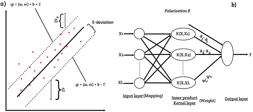
Figure 1. Gaussian support vector regression (GSVR) framework (A) scatter-space diagram and (B) layout diagram.

Conversely, Multilinear regression (MLR) and analysis of variance (ANOVA) are both important statistical techniques used in data analysis and modeling, particularly in the context of understanding relationships between variables and assessing the significance of these relationships. Multilinear regression is a statistical technique that extends simple linear regression to incorporate multiple independent variables to predict a dependent variable. Multilinear regression (MLR) and analysis of variance (ANOVA) are both important statistical techniques used in data analysis and modeling, particularly in the context of understanding relationships between variables and assessing the significance of these relationships. Multilinear regression is a statistical technique that extends simple linear regression to incorporate multiple independent variables to predict a dependent variable Y. In summary, MLR is a method used to model the relationship between a dependent variable and multiple independent variables, while ANOVA is a technique used to assess differences among group means. In the context of MLR, ANOVA serves as a tool for assessing the overall and individual significance of the model and its predictors.

2.2 Deployed performance indices (MSE, MAE, MAPE, RMSE, and R²)

The MSE (Mean Squared Error), MAE (Mean Absolute Error), MAPE (Mean Absolute Percentage Error), RMSE (Root Mean Squared Error), and R-squared (Coefficient of Determination) are widely used metrics in regression analysis. Here’s a brief overview of the significance of each metric: 1. Mean Squared Error (MSE): The MSE measures the average squared difference between the predicted values and the actual values in a regression model. It penalizes large errors more heavily than smaller ones due to the squaring operation. A lower MSE indicates better accuracy and goodness of fit. 2. Mean Absolute Error (MAE): The MAE measures the average absolute difference between the predicted values and the actual values. It provides a more interpretable measure of error compared to MSE as it is in the original scale of the data. Like MSE, a lower MAE indicates better accuracy. 3. Mean Absolute Percentage Error (MAPE): The MAPE measures the average percentage difference between the predicted values and the actual values. It is useful when you want to assess the relative error in terms of percentages. However, MAPE can be problematic when the actual values are close to zero, as it can result in division by zero or extremely large errors. 4. Root Mean Squared Error (RMSE): The RMSE is the square root of the MSE, and it represents the typical magnitude of the residuals or prediction errors. Like MSE, a lower RMSE indicates better accuracy. RMSE is often preferred when you want to report errors in the same unit as the dependent variable. 5. R-squared (Coefficient of Determination): R-squared measures the proportion of the variance in the dependent variable that is predictable from the independent variables in a regression model. It ranges from 0 to 1, where a higher value indicates a better fit. R-squared provides information about the goodness of fit of the model but does not indicate the accuracy of individual predictions. In summary, MSE, MAE, MAPE, RMSE, and R-squared are important metrics in regression analysis that provide insights into the accuracy, goodness of fit, and relative error of the model. It is recommended to use multiple metrics to have a comprehensive understanding of the model’s performance.

Here, Equations 16–20 are the formulas for calculating Mean Squared Error (MSE), Mean Absolute Error (MAE), Mean Absolute Percentage Error (MAPE), Root Mean Squared Error (RMSE), and R-squared (R²):

(a) Mean Squared Error (MSE):

$\text{MSE}=\left(1/\mathrm{n}\right)\mathrm{x}{\displaystyle \sum }{\left({\mathrm{y}}_i-\mathrm{ȳ}\right)}^2(16)$

where: - n is the number of samples. - y_i is the observed value of the i-th sample. - ȳ is the predicted value of the i-th sample.

(b) Mean Absolute Error (MAE):

$\text{MAE}=\left(1/\mathrm{n}\right)\mathrm{x}{\displaystyle \sum }\left({\mathrm{y}}_i-\mathrm{ȳ}\right)(17)$

where: - n is the number of samples. - y_i is the observed value of the i-th sample. - ȳ is the predicted value of the i-th sample.

(c) Mean Absolute Percentage Error (MAPE):

$\text{MAPE}=\left(1/\mathrm{n}\right)\mathrm{x}{\displaystyle \sum }\left[\left({\mathrm{y}}_i-\mathrm{ȳ}\right)/{\mathrm{y}}_{\mathrm{i}}\right]\mathrm{x}100(18)$

where: - n is the number of samples.- y_i is the observed value of the i-th sample.- ȳ is the predicted value of the i-th sample.

(d) Root Mean Squared Error (RMSE):

$\text{RMSE}=\sqrt{\left(\text{MSE}\right)}(19)$

where MSE is the Mean Squared Error.

(e) R-squared (R²):

${\mathrm{R}}^2=1-\left(\text{SSR\hspace{0.17em}}/\text{\hspace{0.17em}SST}\right)(20)$

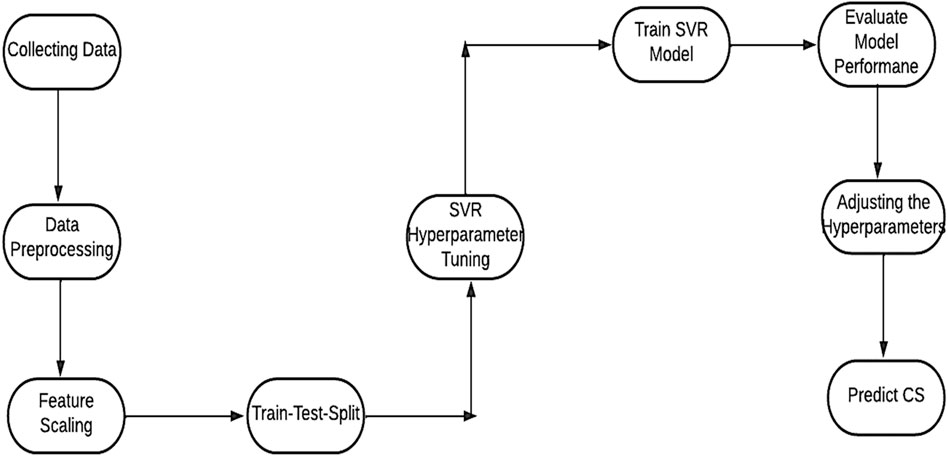
where: - SSR (Sum of Squared Residuals) = Σ(y_i - ȳ)² - SST (Total Sum of Squares) = Σ(y_i - ȳ̄)²- y_i is the observed value of the i-th sample. - ȳ is the predicted value of the i-th sample. - ȳ is the mean of the observed values. It is important to note that the above formulas assume a regression context, where y_i represents the actual values and ȳ represents the predicted values. The SVR flowchart is as presented in Figure 2.

Figure 2

Figure 2. The SVR flowchart.

2.3 Sensitivity analysis

Sensitivity analysis refers to the process of quantifying the impact of changes in input variables on the output of a model or system. It helps assess the robustness and stability of the model’s results. There are various methods for conducting sensitivity analysis, and different formulas may be used based on the specific technique employed. Here, I’ll describe two common methods along with their formulas:

1. One-Way Sensitivity Analysis: In one-way sensitivity analysis, the impact of varying one input variable while keeping others constant is analyzed. The formula for calculating the sensitivity index or the percentage change in the output per unit change in the input variable is given by:

$\text{Sensitivity\hspace{0.17em}Index}=\left(\text{Dy}/\text{Dx}\right)\mathrm{x}\left(\mathrm{x}/\mathrm{y}\right)(21)$

where: - Dy/Dx represents the change in the output variable (y) per unit change in the input variable (x). - x represents the input variable. - y represents the output variable.

2. Tornado Diagram: The tornado diagram is a graphical representation of sensitivity analysis that shows the relative importance of input variables. The formula for calculating the sensitivity index for each variable is the same as the one-way sensitivity analysis method in Equation 21. The sensitivity index is calculated for each input variable, and the variables are ranked based on the magnitude of their sensitivity indices. It is important to note that sensitivity analysis can be much more complex depending on the nature of the model and the specific analysis being conducted. The formulas provided above represent simplified versions for one-way sensitivity analysis and tornado diagram, respectively.

3 Results and analysis

3.1 Statistical and regression analysis

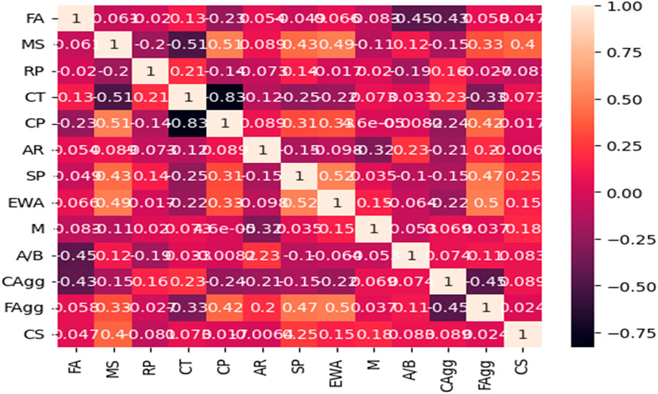
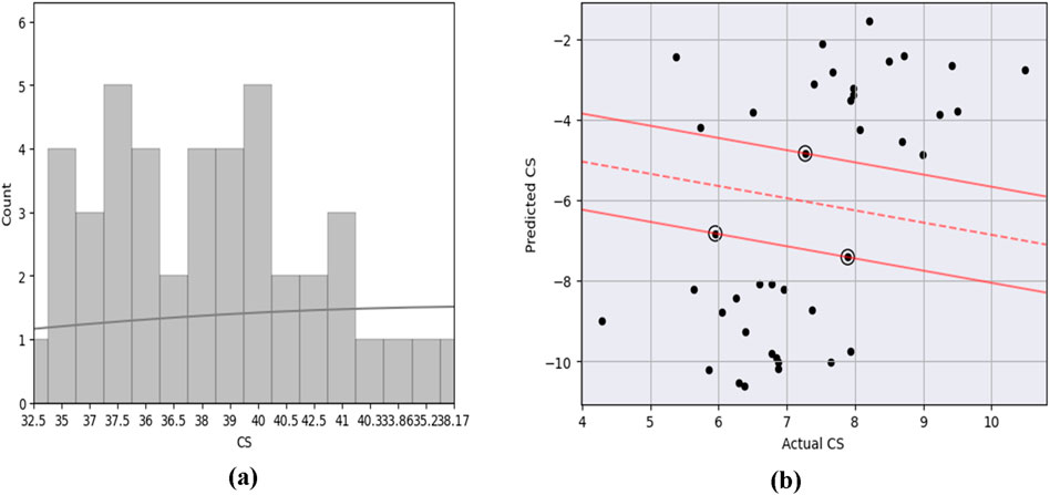
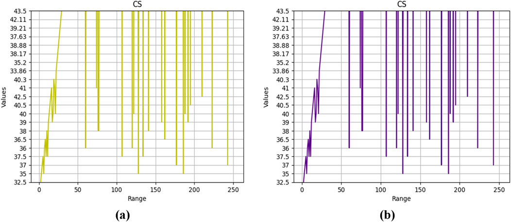
Figure 3 presents the basic linear fittings to determine agreement between the parameters and the Pearson correlation between the studied parameters of the geopolymer concrete. It can be observed that the CS showed very poor correlations with the values of the input parameters and required an improvement of the internal consistency of the dataset to achieve a good model performance. This necessitated the deployment of the super-hybrid interface between the GSVR and the XGB. Figure 4 presented the frequency histogram and the Gaussian support vector machine architecture for the output (CS). This shows serious outliers in the support vector machine which were tuned by using the boosting algorithm combined in the computation interface to enhance the GSVR hyperplane. This eventually produced a super-performance and execution speed remarkable for its use in the forecasting of the compressive strength (CS) of the high-strength geopolymer concrete for sustainable concrete design, production and placement during construction activities.

Figure 3

Figure 3. Pearson correlation between the studied parameters of the geopolymer concrete.

Figure 4

Figure 4. (A) Frequency histogram and (B) the support vector machine architecture for the output.

3.2 Measure of the performance indices

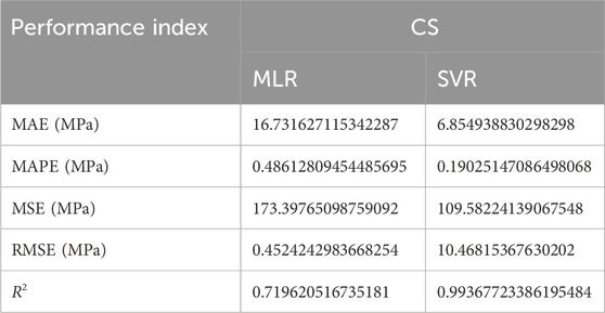
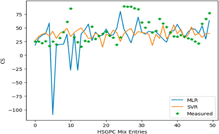
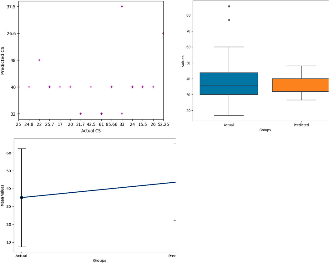
In Figure 5 and Table 1, the measure of the performance evaluation in comparison between measured and predicted values are presented on the basis of the MAE, MSE, RMSE, MAPE and R² for the MLR and the SVR. It can be observed that the MAE produced 16.731 MPa, MSE produced 173.398 MPa, RMSE produced 0.452 MPa, MAPE produced 0.486 MPa and with R² of 0.720 for the MLR and the MAE produced 6.855 MPa, MSE produced 109.582 MPa, RMSE produced 10.468 MPa, MAPE produced 0.190 MPa and with R² of 0.994. These results show the super-performance display of the hybrid algorithms of the Gaussian support vector regression (GSVR) and the extreme gradient boosting (XGBoosting), which produced a superior and decisive model with excellent output compared to the MLR. Also, the execution time reduced from a 24-hour runtime to 1-hour runtime, which reduced the time and energy utilized in the model execution. Also, the GSVR-XGB produced minimal errors as presented in Figure 5 and Table 1. Figure 6 shows the comparison between the MLR, GSVR-XGB, and Measured values. It can be seen that the GSVR produced values optimized to match the measured values better than the MLR. This shows how closely correlated the hybrid model is to the measured values in a more consistent relationship. Figure 7 shows the ANOVA representation of the comparison between the measured and predicted values of the strength of the studied concrete.

Figure 5

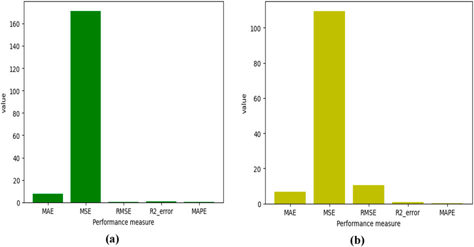
Figure 5. Measure of the performances indices based on MAE, MSE, RMSE, MAPE and R² for (A) MLR and (B) GSVR.

Table 1

Table 1. Performance evaluation in comparison between measured and predicted values.

Figure 6

Figure 6. The comparison of the MLR, SVR, and Measured values.

Figure 7

Figure 7. ANOVA comparison of the predicted and measured values.

3.3 Parametric study and sensitivity analysis

Figures 8, 9 present the parametric study and the sensitivity analyses of the CS studied parameters for the MLR and the GSVR-XGB. Performing a regression parametric study of compressive strength of geopolymer concrete using the Gaussian support vector regression (GSVR) incorporated into the super interface of the XGBoosting involves analyzing the relationship between the input parameters (independent variables) and the compressive strength (dependent variable) using the GSVR and XGB algorithms. A dataset was collected consisting of observations of geopolymer concrete samples. Each observation included the values of the input parameters (e.g., composition, curing time, temperature) and the corresponding compressive strength. The dataset was preprocessed by handling missing values, data normalization, and feature scaling where necessary. GSVR is sensitive to the scale of the input data, so it was important to ensure that the input variables are on a similar scale. The dataset was split into training and testing subsets. The training set was used to train the GSVR model, while the testing set was used for evaluating the model’s performance. GSVR model was trained on the training dataset. GSVR is a machine learning algorithm that learns the relationship between the input parameters and the compressive strength employing the Gaussian kernel function. It aims to find an optimal hyperplane that maximizes the margin while minimizing the error. The trained GSVR model was evaluated using the testing dataset. The predicted compressive strength values were calculated using the model and compared with the actual values. Appropriate evaluation metrics such as MSE, MAE, RMSE, or R-squared were used to assess the model’s performance. The parametric study was conducted by analyzing the impact of individual input parameters on the compressive strength. This was done by systematically varying one parameter while keeping others constant and observing the corresponding changes in the predicted compressive strength. The results of the parametric study are presented in Figure 9 to understudy the influence of each input parameter on the compressive strength. The significant parameters that have a substantial effect on the outcome can be identified as AR and EWA for the MLR and the GSVR-XGB as presented in Figures 9A, B, respectively and this presents insights into the behavior of geopolymer concrete with respect to the influential factors. This supports the concept that the extra water added (EWA) was needed to improve hydration and geopolymerization reactions in the geopolymer concrete (GPC) structural behavior. It is important to note that the impacts of the studied variables may vary depending on the GSVR-XGB implementation and the characteristics of the geopolymer concrete dataset (Ahmad et al., 2022).

Figure 8

Figure 8. The parametric study of the CS studied parameters for (A) MLR and (B) SVR.

Figure 9

Figure 9. The sensitivity analyses of the CS w.r.t. the input parameter for (A) MLR and (B) GSVR.

4 Conclusion

The quintenary influence of industrial wastes comprising fly ash (FA) and metallurgical slag (MS) on the compressive strength of high-strength geopolymer concrete under different curing regimes for sustainable structures has been studied with the deployment of the Gaussian support vector regression optimized with extreme gradient boosting algorithms to form the GSVR-XGBoost hybrid model. Rest time (RP), curing temperature (CT), superplasticizer (SP), alkali ratio (AR), extra water added (EWA), alkali molarity (M), alkali/binder ratio (A/B), coarse and fine aggregates were also considered as factors in the production of the high strength geopolymer concrete (HSGPC). The compressive strength of the HSGPC was tested as the output in the machine learning exercise, which optimized the utilization of the industrial waste in the production of the studied concrete. Multiple mixes of this concrete were studied to produce data entries corresponding to these parameters. The following can be concluded from the research exercise;

• The influence of the industrial wastes, FA and MS in the concrete mixes showed improvement in the compressive strength as shown in the strength responses with the addition of different dosages of FA and MS in the measured concrete mixes.

• The GSVR-XGBoost performed the model run with a speed higher than the normal gaussian-trained support vector regression (GSVR) due to the algorithmic boosting it received in the hybrid interface.

• The GSVR-XGBoost outclassed the MLR and previous works which had used other ML techniques on the same database as presented in the results discussion.

• The GSVR-XGBoost showed closer consistent predicted values compared to the measured values than the MLR, and this shows the decisive ability of the hybrid SVR in combination with XGB.

• The GSVR-XGBoost proved to be a decisive modeling tool for the prediction of the compressive strength of the HSGPC for the data range used on this research work beyond which a quick adjustment is required.

• However, the developed technique is valid within the considered range of each input parameter and it should be verified beyond these ranges. It is thus recommended that other machine learning methods be applied to the reported database to check model performance gaps.

Data availability statement

The original contributions presented in the study are included in the article/Supplementary Material, further inquiries can be directed to the corresponding author.

Author contributions

CG: Data curation, Investigation, Methodology, Validation, Visualization, Writing–review and editing. AA: Formal Analysis, Investigation, Methodology, Project administration, Resources, Validation, Writing–review and editing. SH: Investigation, Methodology, Project administration, Writing–review and editing. KO: Conceptualization, Data curation, Formal Analysis, Methodology, Software, Supervision, Validation, Visualization, Writing–original draft, Writing–review and editing. HI: Data curation, Formal Analysis, Investigation, Resources, Writing–review and editing. SH: Investigation, Methodology, Project administration, Resources, Writing–review and editing. BC: Data curation, Formal Analysis, Investigation, Methodology, Project administration, Writing–review and editing. MV: Data curation, Writing–review and editing.

Funding

The authors declare that no financial support was received for the research, authorship, and/or publication of this article.

Conflict of interest

The authors declare that the research was conducted in the absence of any commercial or financial relationships that could be construed as a potential conflict of interest.

Publisher’s note

All claims expressed in this article are solely those of the authors and do not necessarily represent those of their affiliated organizations, or those of the publisher, the editors and the reviewers. Any product that may be evaluated in this article, or claim that may be made by its manufacturer, is not guaranteed or endorsed by the publisher.

Supplementary material

The Supplementary Material for this article can be found online at: https://www.frontiersin.org/articles/10.3389/fbuil.2024.1433069/full#supplementary-material

References

Ahmad, A., Ahmad, W., Aslam, F., and Joyklad, P. (2022). Compressive strength prediction of fly ash-based geopolymer concrete via advanced machine learning techniques. Case Stud. Constr. Mater. 16, e00840. doi:10.1016/j.cscm.2021.e00840

CrossRef Full Text | Google Scholar

Ahmad, A., Ahmad, W., Chaiyasarn, K., Ostrowski, K. A., Aslam, F., Zajdel, P., et al. (2021). Prediction of geopolymer concrete compressive strength using novel machine learning algorithms. Polymers 13, 3389. doi:10.3390/polym13193389

PubMed Abstract | CrossRef Full Text | Google Scholar

Ahmadi Maleki, M., and Emami, M. (2019). Application of SVM for investigation of factors affecting compressive strength and consistency of geopolymer concretes. J. Civ. Eng. Mater. Appl. 3 (2), 101–107. doi:10.22034/jcema.2019.92507

CrossRef Full Text | Google Scholar

Ahmed, H. U., Mostafa, R. R., Mohammed, A., Sihag, P., and Qadir, A. (2023). Support vector regression (SVR) and grey wolf optimization (GWO) to predict the compressive strength of GGBFS-based geopolymer concrete. Neural Comput&lic 35, 2909–2926. doi:10.1007/s00521-022-07724-1

CrossRef Full Text | Google Scholar

Albitar, M., Visintin, P., Ali, M. S. M., and Drechsler, M. (2015). Assessing behaviour of fresh and hardened geopolymer concrete mixed with class-F fly ash. KSCE J. Civ. Eng. 19, 1445–1455. doi:10.1007/s12205-014-1254-z

CrossRef Full Text | Google Scholar

Alyousef, R., Ebid, A. A. K., Huseien, G. F., Mohammadhosseini, H., Alabduljabbar, H., Poi Ngian, S., et al. (2022). Effects of sulfate and sulfuric acid on efficiency of geopolymers as concrete repair materials. Gels 8, 53. doi:10.3390/gels8010053

PubMed Abstract | CrossRef Full Text | Google Scholar

Ebid, A. M., Onyelowe, K. C., and Deifalla, A. F. (2023a). “Data utilization and partitioning for machine learning applications in civil engineering,” in Conference: International Conference on Advanced Technologies for Humanity, ICATH, Rabat, Morocco, December 25–26, 2023, 25–26.

Google Scholar

Ebid, A. M., Onyelowe, K. C., Kontoni, D. P. N., Gallardo, A. Q., and Hanandeh, S. (2023b). Heat and mass transfer in different concrete structures: a study of self-compacting concrete and geopolymer concrete. Int. J. Low-Carbon Technol. 18, 404–411. doi:10.1093/ijlct/ctad022

CrossRef Full Text | Google Scholar

Huo, W., Zhu, Z., Sun, H., Ma, B., and Yang, L. (2022). Development of machine learning models for the prediction of the compressive strength of calcium-based geopolymers. J. Clean. Prod. 380 (Part 2), 135159. doi:10.1016/j.jclepro.2022.135159

CrossRef Full Text | Google Scholar

Imtiaz, L., Rehman, S. K. U., Memon, A. S., Khizar, K. M., and Faisal, J. M. (2020). A review of recent developments and advances in eco- friendly geopolymer concrete. Appl. Sci. 10, 7838. doi:10.3390/app10217838

CrossRef Full Text | Google Scholar

Khan, M. A., Zafar, A., Farooq, F., Javed, M. F., Alyousef, R., Alabduljabbar, H., et al. (2021). Geopolymer concrete compressive strength via artificial neural network, adaptive neuro fuzzy interface system, and gene expression programming with K-fold cross validation. Front. Mater. 8, 621163. doi:10.3389/fmats.2021.621163

CrossRef Full Text | Google Scholar

Kumar, A., Sinha, S., Saurav, S., and Chauhan, V. B. (2023). Prediction of unconfined compressive strength of cement–fly ash stabilized soil using support vector machines. Asian J. Civ. Eng. 25, 1149–1161. doi:10.1007/s42107-023-00833-9

CrossRef Full Text | Google Scholar

Marangu, J. (2020). Prediction of compressive strength of calcined clay based cement mortars using support vector machine and artificial neural network techniques. J. Sustain. Constr. Mater. Technol. 5 (1), 392–398. doi:10.29187/jscmt.2020.43

CrossRef Full Text | Google Scholar

Onyelowe, K. C., Mahesh, C. B., Srikanth, B., Nwa-David, C., Obimba-Wogu, J., and Shakeri, J. (2021). Support vector machine (SVM) prediction of coefficients of curvature and uniformity of hybrid cement modified unsaturated soil with NQF inclusion. Clean. Eng. Technol. 5, 100290. doi:10.1016/j.clet.2021.100290

CrossRef Full Text | Google Scholar

Onyelowe, K. C., Onyia, M. E., Bui Van, D., Baykara, H., and Ugwu, H. U. (2021a). Pozzolanic reaction in clayey soils for stabilization purposes: a classical overview of sustainable transport geotechnics. Adv. Mater. Sci. Eng. 2021. 7. doi:10.1155/2021/6632171

CrossRef Full Text | Google Scholar

Qaidi, S. M. A., Tayeh, B. A., Isleem, H. F., de Azevedo, A. R. G., Ahmed, H. U., and Emad, W. (2022a). RETRACTED: sustainable utilization of red mud waste (bauxite residue) and slag for the production of geopolymer composites: a review. Case Stud. Constr. Mater. 16, e00994. doi:10.1016/j.cscm.2022.e00994

CrossRef Full Text | Google Scholar

Qaidi, S. M. A., Tayeh, B. A., Zeyad, A. M., de Azevedo, A. R. G., Ahmed, H. U., and Emad, W. (2022b). Recycling of mine tailings for the geopolymers production: a systematic review. Case Stud. Constr. Mater. 16, e00933. doi:10.1016/j.cscm.2022.e00933

CrossRef Full Text | Google Scholar

Sathiparan, N., and Jeyananthan, P. (2023). Predicting compressive strength of cement-stabilized earth blocks using machine learning models incorporating cement content, ultrasonic pulse velocity, and electrical resistivity. Nondestruct. Test. Eval. 39, 1045–1069. doi:10.1080/10589759.2023.2240940

CrossRef Full Text | Google Scholar

Silva, P., Moita, G., and Arruda, V. (2020). Machine learning techniques to predict the compressive strength of concrete. Rev. Int. Métodosnumér. Cálc. Diseñoing. 36 (4). doi:10.23967/j.rimni.2020.09.008

CrossRef Full Text | Google Scholar

Sobhani, J., Khanzadi, M., and Ovahedian, A. H. (2013). Support vector machine for prediction of the compressive strength of no-slump concrete. Comput. Concr. 11 (4), 337–350. doi:10.12989/CAC.2013.11.4.337

CrossRef Full Text | Google Scholar

Tran, V. Q. (2023). Data-driven approach for investigating and predicting of compressive strength of fly ash–slaggeopolymerconcrete. Struct. Concr. 24, 7419–7444. doi:10.1002/suco.202300298

CrossRef Full Text | Google Scholar

Verma, M., and Dev, N. (2021). Sodium hydroxide effect on the mechanical properties of fly ash-slag based geopolymer concrete. Struct. Concr. 22 (S1), E368–E379. ISSN: 1751-7648. doi:10.1002/suco.202000068

CrossRef Full Text | Google Scholar

Zhang, D., Sun, F., and Liu, T. (2021). Prediction of compressive strength of geopolymer concrete based on support vector machine and modified cuckoo algorithm. Adv. Mater. Sci. Eng. 24. 1–14. doi:10.1155/2021/4286810

CrossRef Full Text | Google Scholar