 Bashar Al Shawa
- Joule Consulting Group, Bath, United Kingdom
To align the buildings sector with the 1.5°C climate change trajectory, enormous improvements in energy efficiency are needed. It is therefore crucial that the tools used to evaluate buildings’ energy use undergo robust testing. This paper tests, for the first time, the outcome of the Passive House Planning Package (PHPP) and an author-modified version of the Radiant Time Series Method (RTSM), following the Building Energy Simulation Test (BESTEST). The results show that while the validity of the modified-RTSM is slightly superior to that of the PHPP, both tools pass less than 35% of the cases—necessitating further calibration and challenging the widely-held belief that the PHPP is ‘validated’. As the PHPP and the modified-RTSM present a relatively simple and quick way of evaluating buildings’ energy performance, calibrating their methodologies so they pass the BESTEST cases could put them at an advantage over the fully dynamic and resource-intensive tools.
1 Introduction
The buildings sector is responsible for 30% of the world’s final energy consumption and 27% of global energy-related emissions (IEA, 2022a). Although various building energy codes and standards were introduced in recent years, the sector’s total energy demand and energy-related CO2 emissions increased by an average of 1.5% and 1.2% per year from 2010 to 2021 (IEA, 2022a; UNEP, 2022). The International Energy Agency (IEA) describes the sector as being “not on-track” to meet its deliverables under the Net Zero Emissions by 2050 Scenario—a scenario that offers a 50% chance of limiting the rise in global temperatures at 1.5°C above pre-industrial levels (IEA, 2021).
There are several factors implicated for this shortcoming. One such factor is the significant expansion of the sector’s built-up area, which has increased by 1.9% per year from 2010 to 2021 and is expected to almost double by 2060 (IEA, 2022b; 2017). Another factor is the sector’s ‘performance gap’—where a building’s calculated energy demand is different from that measured. This gap varies greatly and can be in either direction. For instance, a review by Shi et al. (2019) shows that the ratio between a building’s measured energy demand and that predicted can range from as little as 0.29 (i.e., where a building consumes less than predicted) to a substantial 4.0 (where a building consumes four times more than predicted).
The factors leading to this gap can be classified as either socioeconomic or technical and, in many instances, both types would be acting simultaneously. Socioeconomic factors include the rebound effect, where an improvement in the energy efficiency of a service leads to a less-than-predicted energy saving—and sometimes a higher energy consumption—due to the reduction in the perceived price of that service (Saunders, 1992). Within the buildings sector, this is estimated to range from 6% to a substantial 187%—meaning that 6%–187% of the predicted energy savings are not realised (Al Shawa, 2022). Another socioeconomic phenomenon is the income elasticity of energy demand—i.e., the percentage increase in energy demand with every 1% increase in income. Within the buildings sector, this ranges from 0.11 to 2.94—indicating that with every 1% increase in income, there could be a 0.11%–2.94% increase in energy demand.
The technical causes of the performance gap are several, and it is difficult the quantify the magnitude of each as they often act concurrently. For instance, poor construction quality is often cited as such cause, which is where the thermal performance of the delivered building does not match that assumed during the design stage. For instance, Asdrubali et al. (2014) compared the measured U-values of six external walls with those assumed in the energy models of various buildings in central Italy. They conclude that, in five of the six walls, the measured U-values were 15%–43% higher than those assumed in the energy model. Johnston et al. (2015) reach a similar conclusion for dwellings in the UK, where the measured U-values were approximately 60% higher than those assumed in the design stage’s energy model.
Another technical cause is the accuracy of the weather data used to predict the energy performance of a building. A study by Bhandari et al. (2012) analysed the difference between weather data supplied by two providers and that measured on-site in Oak Ridge, United States. They show that a variation of up to 90% can occur for a single variable, leading to a difference of up to 7% in building energy consumption and up to 90% in peak loads. Confirming these findings, Wang et al. (2012) compared the outcome of an EnergyPlus simulation using actual weather data and that using a Typical Meteorological Year (TMY3) weather file, and show that a variation of up to 6% can occur in building energy use.
Lastly, a third factor is building energy simulation programmes themselves. This includes their inherent simplification of various thermodynamic interactions occurring within buildings which, sometimes, limits their ability to accurately model unconventional heating, cooling, and air conditioning systems (Salehi et al., 2013), natural ventilation (Crawley et al., 2008), and complex building geometry (Herrando et al., 2016). This also includes whether a specific programme or methodology has undergone a robust testing procedure (Crawley et al., 2008) and if it did, how well it faired. It is this last factor that is the main focus of this paper, and which will be discussed in detail in the subsequent sections.
1.1 Verification, validation, and comparative testing of building energy simulation tools
Since their inception more than 50 years ago (Crawley et al., 2008), the number of building energy simulation tools has proliferated (Rittelmann and Ahmed, 1985). At the time, no robust procedures that can test the validity of these tools’ output had existed. Research conducted by the National Renewable Energy Laboratory (NREL, then called Solar Energy Research Institute) noted considerable unexplained differences between the output of four simulation tools—namely: DOE-2, BLAST, DEROB, and SUNCAT. In recognition of these discrepancies, the International Energy Agency (IEA) initiated various workstreams to develop a comprehensive methodology to test the validity of these tools. This included the Solar Heating and Cooling (SHC) tasks 8 and 12 established in 1977 (Judkoff and Neymark, 1995a).
At the most basic level, a tool is usually tested by comparing its annual output with a measured value. This approach is often preferred by tool developers as it mimics the way in which a tool would be used in reality (i.e., to predict the annual energy consumption of a building). However, such an approach does not isolate the multiple sources of potential error that could be acting simultaneously. Therefore, even if a tool correctly predicts a building’s annual energy consumption, it is possible that, due to compensating errors, that correct prediction is due to an internal error in the tool’s algorithm. Recognising this, the NREL developed a robust methodology for testing building energy simulation tools which could—to an extent—eliminate compensating errors and isolate the potential source(s) of error. Broadly speaking, the methodology starts with the simplest case and then changes a single parameter with each case, and the tests are conducted under various climates, building types, and modes of operation. The methodology proposed by the NREL was generally accepted by the IEA and has formed the basis for the various types of tests that were developed later on (Judkoff and Neymark, 1995a).
The tests stemming from that methodology often taken one of three forms: A) verification—where a tool’s ability to correctly perform its intended algorithm is tested; B) empirical validation—where the output of a tool is compared against measured physical phenomena; and C) comparative testing—where the output of a tool is compared with that of other tools (Judkoff and Neymark, 1995a; Trucano et al., 2006). Since 1980, both the NREL and the IEA have developed various tests for each of these three types. For instance, several tests were developed to verify a tool’s analytical solution for various problems such as wall conduction, mass charging, and infiltration. Tools that have undergone these tests include DEROB-3/4, DOE2.1, BLAST-3, and SUNCAT-2.4. In terms of empirical validation, an experiment was carried out where various tests cells were built in Denver (United States), Los Alamos (United States), and Ottawa (Canada), and the output of several simulation tools was then compared with the measured data of these cells. Lastly, comparative testing was initiated through IEA’s Solar Heating and Cooling (SHC) Task 12 and culminated in the development of the Building Energy Simulation Test (BESTEST) by NREL (Judkoff and Neymark, 1995a). BESTEST, in turn, formed the basis for the American Society of Heating, Refrigerating, and Air-conditioning Engineers’ (ASHRAE) (ASHRAE Standard 140-2011, 2011) —which is considered today as one of the most rigorous and widely-used software testing procedures (Judkoff and Neymark, 2013).
The BESTEST standard comprises a series of carefully selected test cases that assess a tool’s ability to model various phenomena, including conduction, infiltration, internal heat gain, solar transmission and incidence, and thermal mass. Eight public domain dynamic simulation tools (the definition of which is further explained in Section 1.3) from the United States and Europe were employed to run various test cases and their results were presented in the standard. The simulation tools that were employed are shown in Table 1.
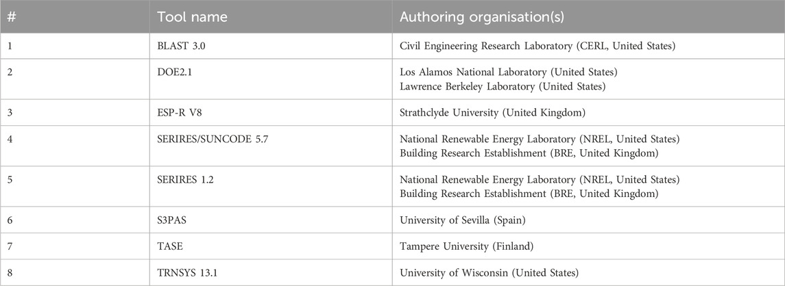
Table 1. The eight simulation tools used in the BESTEST standard (Judkoff and Neymark, 1995a).
While the range of results established by these tools does not constitute the “truth”, it does represent the results of state-of-the-art simulation tools that have been calibrated, scrutinised, and empirically validated over the past 50 years. Therefore, the result of a tool or a methodology falling outside that range does not necessarily mean it is incorrect, but it does merit the need for further calibration. The intention of the BESTEST standard is to assess the suitability of a simulation tool to run a particular problem and, based on the outcome, give the design and engineering communities a degree of confidence in that tool. While this may not be a perfect solution, it is a better approach when compared with using simulation tools “on blind faith” (Judkoff and Neymark, 1995a).
Having provided a brief introduction on the various methods and procedures used to test the robustness of building simulation tools, the paper will now discuss the degree to which two of these tools have been scrutinised. Namely, the Passive House Planning Package (PHPP) and the Radiant Time Series Method (RTSM). The selection of these two tools, rather than others, mainly stems from their popularity and their ability to estimate heating and cooling demands in a relatively simple and quick manner, as is further explained in the following sections 1.2 and 1.3.
1.2 Passive House Planning Package (PHPP)
Passivhaus is a German building energy efficiency standard developed by the Passive House Institute in 1990. It is based on a fabric-first approach and, through the efficient use of solar and internal heat gains and heat recovery, buildings designed to the Passivhaus criteria consume up to 75% less energy compared with a typical new build (Passive House Institute, 2019a). To date, there are more than 5,300 certified Passivhaus buildings worldwide, located across Europe, North America, Latin America, Africa, Asia, the Middle East, and the South Pacific. Compliance with the Passivhaus standard is now also mandated in various provinces around the world, including New South Wales (Australia), Vorarlberg (Austria), and Brussels and Antwerp (Belgium) (International Passive House Association, 2024).
All buildings seeking certification under the Passivhaus standard must demonstrate compliance through Passivhaus’ modelling tool—the Passive House Planning Package (PHPP) (Passivhaus Trust UK, 2024a). The PHPP is an energy balance tool introduced by the Passive House Institute in 1998 and has since undergone continuous development. It is an Excel-based tool comprising various inputs, and it enables designers to quickly assess the effect of various design interventions on a building’s energy consumption, peak loads, and thermal comfort.
The energy calculation engine of PHPP’s older versions (up to version 9) was based on the International Standardisation Organisation (ISO) Standard 13790’s monthly method, whereas that of the current version 10 is based on ISO 52016’s monthly method (Passive House Institute, 2019b; Passive House Institute, 2021). Current research demonstrates that there is little discernible difference between the two ISO standards (van Dijk, 2018) and, similar to the Radiant Time Series Method (RTSM) that will be discussed in the following Section 1.3, both methods can be considered as quasi-steady state (Kim et al., 2013). The quasi-steady state method, in turn, is where the dynamic effect of quantities such as internal temperature and heat flow rates—which would otherwise be constant over time under the steady state method—vary through the use of correction and adjustment factors derived from a large number of dynamic simulations (van Dijk, 2018; Corrado and Fabrizio, 2019). An important limitation of both the steady and quasi-steady state methods—and one that is apparent in the PHPP—is that the climatic data is processed based on average monthly or seasonal values, whereas a shorter time step (often hourly) is used in the dynamic method (Corrado and Fabrizio, 2019).
Since its inception, the PHPP was subjected to various tests to measure the accuracy of its output, both directly (i.e., testing the PHPP tool itself) and indirectly (i.e., testing its underlying calculation methodologies—e.g., ISO 13790 for PHPP version 9 and earlier and ISO 52016 for version 10). The first of these tests, which assessed the outcome of the PHPP tool itself, was the Cost Efficient Passive Houses as European Standards (CEPHEUS) study (Feist et al., 2001), where 221 Passivhaus-certified dwellings were built and closely monitored in Germany, Sweden, Austria, Switzerland, and France. The project proved the viability of the Passivhaus concept in that, on average, the measured space heating energy demand of Passivhaus dwellings was 84%–87% lower than that of typical newly built dwellings.
Another study that investigated the accuracy of the predictions made by the PHPP is Mitchell and Natarajan (2020), which analysed the measured performance of 97 Passivhaus-certified dwellings in the United Kingdom. The study highlighted the benefits of the Passivhaus concept in that the average space heating demand of Passivhaus dwellings in the United Kingdom is about one-fifth that of newly built homes.
Both the CEPHEUS project (Feist et al., 2001) and the Mitchell and Natarajan (2020) study are cited by the Passive House Institute as proof of the ‘validity’ of the PHPP (Passive House Institute, 2019b; Passipedia, 2023). But that conclusion is brought into question when closely examining both studies. For instance, in the CEPHEUS project, there is a considerable difference between the measured and PHPP-predicted space heating demand of dwellings located in the Austrian cities of Hörbranz (difference of −75%), Egg (difference of 33%), and Dornbirn (difference of 41%) (Feist et al., 2001). Similarly, in the Mitchell and Natarajan (2020) study, the measured space heating demand can be up to one-tenth (if it is less) and twice (if it is higher) that predicted by PHPP.
Another issue is that, even if the PHPP predictions closely matched the measured values, that would not necessarily validate PHPP’s output given the possibility of multiple sources of error acting concurrently. As discussed in Section 1.1, a more robust validation of the PHPP would be to start from the simplest case and then introduce various changes, one at a time, and assess the difference between the measured and PHPP-predicted values for each case.
Another study, which constitutes comparative testing, is that by Charron (2019) in which PHPP version 9.6 (which is based on ISO 13790’s monthly method (ISO, 2008; Passipedia, 2023)) was tested in accordance with ASHRAE Standard 140-2017 (2017). The study was conducted in accordance with the Class I Test Procedures which, the standard asserts, is suitable for tools that are unable to produce hourly or sub-hourly simulation time steps. The Class I Test Procedures were adapted from the Housing Energy Rating System (HERS) BESTEST, which was developed by the NREL with the intention of certifying residential energy simulation tools. This is as opposed to the Class II Test Procedures, which are based upon the IEA BESTEST discussed in Section 1.1 and which aims to test simulation tools irrespective of their time steps’ resolution. The study shows that the PHPP’s results fall within the 93% confidence interval established by the results of the three reference programmes—in this case, BLAST 3.0, DOE 2.1E, and SERIRES 5.7 (Ron Judkoff and Joel Neymark, 1995)—for all 38 cases except one case (L155A: south-facing overhang), whereby the PHPP underpredicted the annual cooling demand by 9% below the lower limit of the confidence interval (Charron, 2019).
Lastly, two studies were conducted which test PHPP’s underlying calculation methodology. The first one, by Kokogiannakis et al. (2008), compares the output of ISO 13790’s monthly and hourly methods with that of EnergyPlus and ESP-r. Whilst this comparative analysis does not follow the procedure suggested by NREL and thus is prone to various shortcomings (discussed in Section 1.1), it is useful in comparing the output of ISO 13790’s monthly method (upon which PHPP version 9 and earlier is based) to that of two simulation tools that have undergone the BESTEST testing procedure with favourable results (i.e., EnergyPlus and ESP-r) (Strachan et al., 2008; Henninger and Witte, 2010). The comparison shows considerable differences between the monthly method on the one hand and EnergyPlus and ESP-r on the other. For instance, for the Athens climate (case 3), the annual heating energy estimated by the monthly method is 2.7 times and 3 times that estimated by EnergyPlus and ESP-r (respectively). When halving the glass area (case 9), the monthly method’s estimate of the annual cooling energy for Amsterdam climate is twice that estimated by EnergyPlus and ESP-r.
1.3 Radiant Time Series Method (RTSM)
The RTSM was developed by Spitler et al. (1997) based on the Heat Balance Method (HBM). It was proposed as a simpler—yet rigorous—alternative to the HBM as it eliminates the need for iterative calculations required by the HBM and could therefore be executed relatively quickly using a spreadsheet. Since its introduction, it has replaced other simplified methods such as the Cooling Load Temperature Difference method (CLTD) (Spitler et al., 1993) and the Transfer Function Method (TFM) (Mitalas, 1972), and has been published in subsequent ASHRAE handbooks as of 2001 (Jeffrey D. Spitler, 2003; Spitler and Nigusse, 2010). Notably, a survey conducted by Mao (Mao, 2016) in Houston, United States, showed that design professionals still use the RTSM—more so than the relatively complex HBM—for computing buildings’ peak loads. The popularity of the RTSM can also be noted in that it is the method adopted by Autodesk’s Revit MEP modelling suite to estimate heating and cooling loads (Sandberg, 2011)—a programme that currently holds an 11.36% market share of all Building Information Modelling (BIM) and architectural design software (6sense, 2024).
A prominent feature of the RTSM is its reliance on Radiant Time Factors (RTFs) and Conduction Time Factors (CTFs). These are series coefficients, derived from the HBM, which reflect the percentage of an earlier radiant heat gain (in the case of RTFs) or conduction heat gain (in the case of CTFs) that becomes a cooling load during the current hour. The RTF and CTF values, in turn, can be determined in one of three ways: 1) using the default values for various external wall and roof systems (as reported in tables 16, 17, and 20 of ASHRAE Handbook: Fundamentals, Chapter 18 (ASHRAE, 2017b); 2) using the spreadsheets supplied with ASHRAE’s Load Calculation Applications Manual (Spitler, 2014); or 3) using the tool developed by Ipseng and Fisher (2003). It is the second and third methodology (henceforth referred to as “LCAM toolkits” and “Ipseng and Fisher”, respectively) that were used in this paper to determine the RTSM’s respective RTFs and CTFs for each BESTEST case, as is further explained under Section 2.2.
In its original form, the RTSM assumes steady periodic conditions—that is, the thermal conditions of a space at a particular hour during the day are identical to those 24 h and 48 h prior to that hour (ASHRAE, 2017b). Therefore, the RTSM is unable to capture heat gains that ‘start’ 24 h or more prior to a particular day, and which would only become a cooling load on that day. This shortcoming would be more pronounced in heavyweight construction where there is a significant delay in heat input at the exterior surface becoming a heat gain at the interior surface and, ultimately, a cooling load once transferred by convection to a space’s air. This also entails that the internal heat gains of a space are identical irrespective of the day—resulting in inaccuracies when estimating the cooling load of, for example, office buildings where these gains are considerably lower in weekends than on weekdays.
Another limitation of the RTSM relates to the design conditions it adopts. For instance, when calculating the beam normal irradiance and diffuse irradiance, clear sky conditions are assumed. Moreover, it uses the n% monthly design day dry-bulb temperature—that is, the temperature that is not exceeded for more than n% of the time for a particular hour of the month—to derive the hourly dry-bulb temperatures for a day that is then used as the hourly design condition for that month (ASHRAE, 2017a). This is somewhat similar to PHPP’s climate data limitation previously discussed under Section 1.2.
It is these limitations that differentiate the RTSM from the more robust HBM, and they are also the reason why ASHRAE recommends that the RTSM is only used for peak load estimates and not for energy demand predictions (Spitler, 2014). However, these two limitations were addressed by the author—to an extent—through an ‘upgraded’ version of the RTSM that has been tested following the BESTEST procedure, as is further explained in Section 2.2.
Various studies were conducted to validate and compare the results of the RTSM against the more rigorous HBM. Overall, these studies note that the RTSM over-predicts the peak cooling load by up to 44% in zones with large single-pane glazing. Researchers suggest that this difference is mainly due to RTSM’s adiabatic zone assumption—i.e., that surface heat gains are modelled to not escape the space (Spitler and Nigusse, 2010). To address this limitation, several correction approaches were put forward that attempt to model that heat loss and integrate it into the RTSM procedure.
One of these first correction approaches was ASHRAE’s Research Project 1117 (henceforth termed RP-1117), which was carried out in 2002 (Fisher and Spitler, Jeffrey D, 2002). Its objectives were to first validate the RTSM in its then-current form and, secondly, introduce a ‘modified RTSM’ that models the heat lost to the atmosphere and compare the results with the original RTSM. Two test cells were built in Oklahoma State University—one lightweight and one heavyweight—and the cooling loads calculated under different methodologies were compared with measured values. The output of the HBM was the closest to the measured values, with a deviation of less than 15% for all cases. The RP-1117 modified approach showed a significant improvement over the original RTSM, achieving a deviation less than 20% from the HBM. It must be noted that these deviations are under “extreme” conditions (i.e., 50% glazing ratio on west and south façades, with single pane glazing), while under “typical” conditions (i.e., 20% glazing ratio on west façade, with double-pane low emissivity glass) the original RTSM was able to match HBM’s results1 (Fisher and Spitler, Jeffrey D, 2002).
Another approach to correct RTSM’s overprediction was done by Nigusse in 2007 (henceforth called Nigusse (2007) which was published in the ASHRAE Transactions journal of 20102 (Spitler and Nigusse, 2010). The approach takes the form of a dimensionless conductance that is subtracted from a zone’s RTFs, which are then applied to compute the cooling load of a room (Nigusse, 2017). The modified RTSM was compared against the HBM for a wide range of configurations, and the highest over-prediction by the original RTSM was noted in zones with relatively large areas of single pane glazing. In these cases, the Nigusse (2007) approach reduced this over-prediction by nearly 60%, whereas in the more realistic cases (double pane glazing with a 40% glazing ratio) this reduction was approximately 9% (Spitler and Nigusse, 2010).
1.4 Scope and objectives
From the brief review presented in sections 1.2 and 1.3, it is evident that, for the PHPP, while its older version (version 9.6) was subjected to a part of the BESTEST verification process intended for residential buildings (HERS), it has not undergone the BESTEST comparative testing procedure (discussed in Section 1.1) that is intended for all types of buildings and which is considered to be the de facto test for all energy simulation tools.
For the RTSM, because it is a simplified version of the Heat Balance Method (HBM) and can be carried using a spreadsheet, it has considerable potential for optimising buildings’ energy efficiency in a quick and cost-effective manner. Given its steady-periodic condition and the conservative climatic design conditions it assumes (discussed in Section 1.3), it is only suitable—in its current form—for load calculations (rather than load and energy calculations). However, as the author has modified the original RTSM such that it incorporates quasi-steady state periodic conditions and is able to read hourly climatic data from a weather file, it is now possible (and worthy) to test its validity for both load and energy estimations.
In light of the above, the aim of this paper is two-fold. First, using the BESTEST procedure, it tests, for the first time, the claimed ‘validity’ of PHPP version 10.3 for both annual energy and peak load predictions. Second, it introduces a novel upgrade to the RTSM whereby it is transformed to quasi-steady state calculation tool that is able to read hourly weather data and, following that, tests that upgraded version following the same BESTEST procedure. Importantly, this exercise tests the validity of both RTSM’s peak load prediction—i.e., its intended purpose—as well as its annual energy estimation, which is now possible due to the novel upgrade introduced.
The results of this exercise have important implications for both policymakers and design practitioners. For the PHPP, given the popularity of the Passivhaus standard and its adoption by various provinces around the world (as discussed under Section 1.2), the validity of the tool that assesses compliance with that standard is critical in minimising the currently-dominant performance gap within the sector (discussed in Section 1). Notably, it also ensures that the target that these provinces sought to achieve through adopting the Passivhaus standard—e.g., to become aligned with the 1.5°C climate change trajectory—is realised.
Equally, for the RTSM, given its popularity among design professionals for estimating peak heating and cooling loads (as discussed in Section 1.3), its accuracy is vital in ensuring the optimal sizing of Heating, Ventilation, and Air Conditioning (HVAC) equipment and avoiding the considerable ‘energy penalty’ caused by oversized equipment (Chiu and Krarti, 2021). Added to that is that if the RTSM’s novel upgrade introduced in this paper is shown to have ‘passed’ the BESTEST, then that upgraded version would be a viable alternative to the more complex and time-consuming HBM in estimating buildings’ heating and cooling energy demands.
2 Methodology
The BESTEST document used to test the validity of the PHPP and the RTSM—in its author-modified version—is titled IEA Building Energy Simulation Test (BESTEST) and Diagnostic Method and is written by Judkoff and Neymark (1995a).
The weather data for the tests cases is available within BESTEST’s supplementary material and has been downloaded from the NREL website (Judkoff and Neymark, 1995b). The weather data is for the City of Denver, Colorado, United States, and is available in a Typical Meteorological Year (TMY) weather data type.
The BESTEST document recommends that a tool runs both the qualification cases (600 and 900 series) as well as the sensitivity cases. In order to test the tools’ ability to model surface convection, infiltration, internal heat gain, and exterior and interior shortwave absorptivity (respectively), four more cases were added: 400, 410, 420, 430, and 440. While the BESTEST document does not set a clear passing criteria for a tool3, it does state that “[a] program may be thought of having passed successfully […] when its results compare favourably with the reference program output”. Therefore, and in-line with what the majority of current building simulation tools have done when running the BESTEST cases (Strachan et al., 2008; Henninger and Witte, 2010, p. 140; Florida Solar Energy Center, 2012; IES, 2018; DesignBuilder, 2019; Trane Technologies, 2020; Carier, 2023; EDSL Tas, 2024), passing a BESTEST case in this paper entails that the tool’s result falls within the range of output established by the BESTEST reference programmes (shown in Table 1). A summary of the BESTEST cases included in this exercise, their parameters, and a three-dimensional view of them is provided in Table 3 and Figure 1.
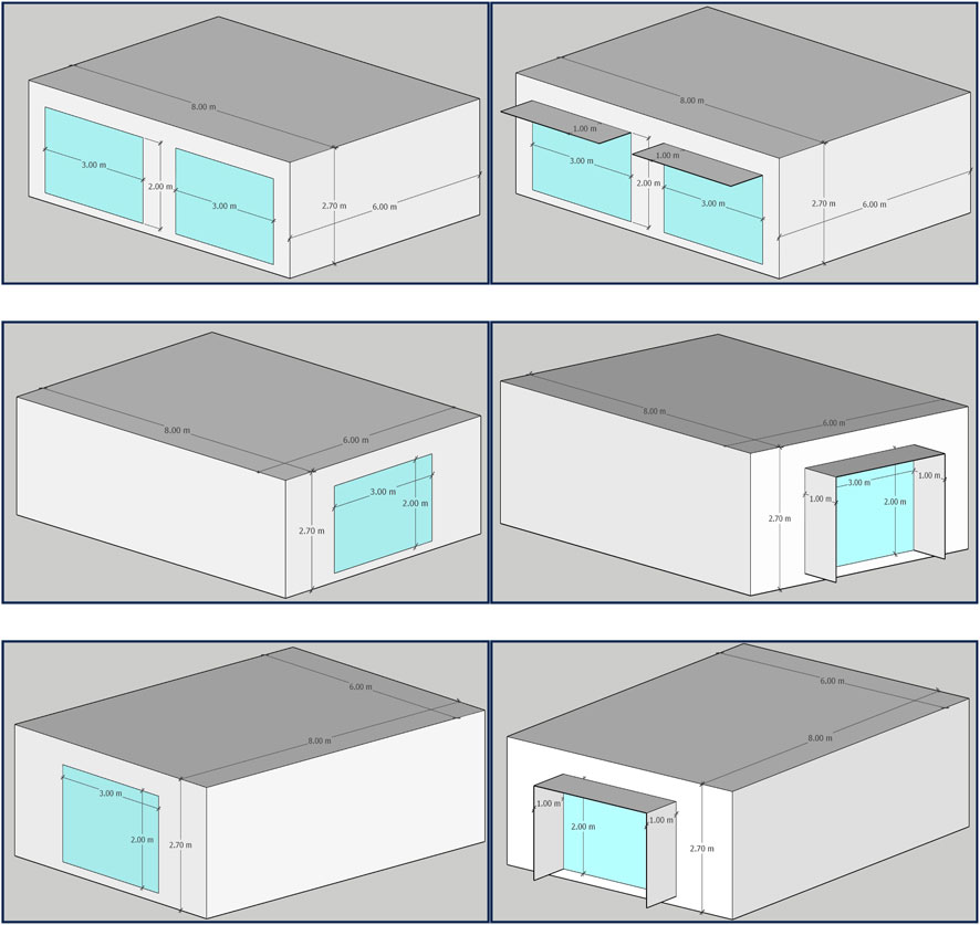
Figure 1. A three-dimensional view of the BESTEST cases included in this exercise. Top row: South-North orientation, no shading (left), with 1 m horizontal shade (right). Middle row: East-West orientation, east elevation, no shading (left), with 1 m horizontal and 1 m vertical shade (right). Bottom row: East-West orientation, west elevation, no shade (left), with 1 m horizontal and 1 m vertical shade (right).
The following Section 2.1 and Section 2.2 discuss which cases each of the tools (PHPP and RTSM) was able to model, along with how both tools were set up to run these cases and the various parameters set.
2.1 PHPP
For running the BESTEST cases, version 10.3 of the PHPP was used. For the climate data, the BESTEST TMY weather file was first converted to an EnergyPlus Weather File (EPW) and then imported into Meteonorm version 8.0.3 (Meteonorm, 2024). From there, the weather data was exported into a PHPP format and then manually entered into the Climate sheet of the PHPP spreadsheet. It is worth noting here that Meteonorm is regularly used by the Passive House Institute and was recommended by the institute as the tool to be used to convert EPW files to PHPP format (Al Shawa, 2023).
To account for the thermal mass of the BESTEST cases, the heat capacity (
where
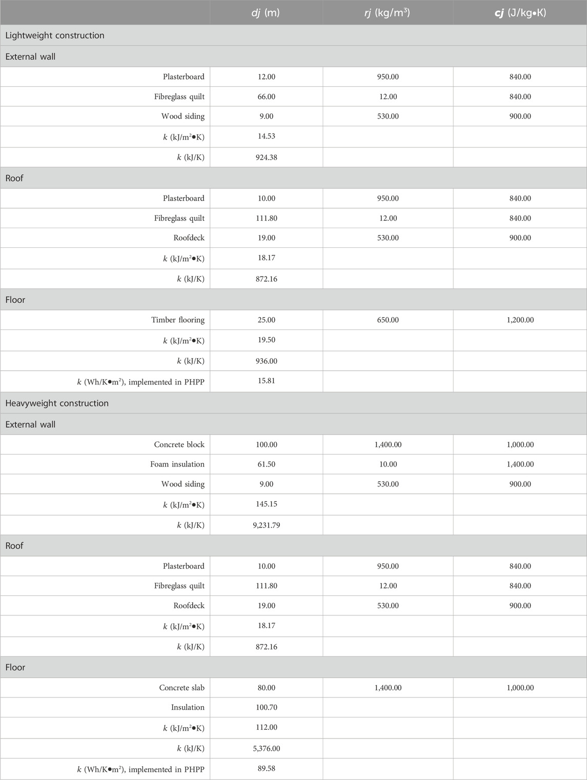
Table 2. The thickness of the layer (

Table 3. The BESTEST cases included in this exercise, along with the parameters of each.
As it is not possible to assign interior shortwave absorptivity values nor heating and cooling setpoints for specific hours in the PHPP, cases 440, 640, 650, 940, and 950 were not modelled.
It is important to note that due to the windows’ dirt factor in the PHPP being fixed at 0.95 with no possibility of changing it, it is likely that the official release of PHPP is unable to perfectly model the solar gain into the interior space as required by BESTEST. This extends to the internal heat gains and infiltration rate which, due to PHPP’s inner formulae, would never perfectly match those required by BESTEST. Nonetheless, an attempt has been made by the author to alter these formulae, and the results of this ‘modified’ PHPP version are reported in the paper’s Supplementary Data and briefly discussed in Section 3.
2.2 RTSM
As discussed under Section 1.3, the RTSM’s steady periodic conditions assumption limits its ability to predict heating and cooling energy use. To overcome this, only the first day of the year is assumed to have steady periodic conditions (as it has no previous conditions), and each hour following that would read its preceding conditions for a period of 24 h. This was made possible by altering the algorithm of the original RTSM tool to read weather data for each hour of the year (i.e., 8,760 h) from BESTEST’s TMY weather file (as shown in Eqs 8, 9), rather than reading one value that represents the conditions during a specific hour of the month, as is commonly done in the RTSM (see Section 1.3 and the ASHRAE Handbook: Fundamentals (2017a)). This upgrade also means that both the beam normal irradiance and diffuse horizontal irradiance (W/m2) will now reflect realistic conditions, as opposed to ASHRAE’s clear-sky conditions—the latter of which will undoubtedly result in an overprediction of cooling energy.
Accordingly, and following the RTSM procedure outlined in the relevant ASHRAE guidance (ASHRAE, 2009; Spitler, 2014), the conduction heat gain of an element (wall or roof) (
Then, the radiant cooling load
where
The RP-1117 correction approach (Fisher and Spitler, Jeffrey D, 2002) (discussed in Section 1.3) attempts to model the short-wave radiation heat gain that is lost to the outdoor environment, and then subtracts that from the radiative portion of the conduction gain (
Thus, the first step is to calculate the short-wave heat gain,
where
where
Next, the total short-wave radiation heat that is lost through the windows,
where
Finally, the
For the Nigusse (2007) correction approach, a dimensionless heat conductance (
where
The above demonstrates how the
Following that, the annual heating and cooling energy demand are calculated by summing the hourly loads occurring for all elements for the entire year, as shown in Eqs 10, 11:
where
Except for the changes introduced above, the RTSM procedure implemented in this paper follows that outlined in Chapter 18 of ASHRAE’s Handbook: Fundamentals (2017 version) (ASHRAE, 2009) and Chapter 7 of ASHRAE’s Load Calculation Applications Manual (2014 version) (Spitler, 2014). Notably, certain mistakes4 were discovered in the former standard, and the author has been in dialogue with ASHRAE regarding this matter. It was confirmed by ASHRAE that an erratum will be published5, rectifying the mistakes pointed out (Owen, 2018).
3 Results and discussion
The passing rate for each of the tested methodologies is shown in Figure 2. As can be noted, the passing rate of the RTSM (for all the correction approaches) compares well with the PHPP. Taking all cases (low mass and high mass) and testing for sensitivity and absolute values, the highest passing rate for the RTSM is achieved by the RP-1117 and Nigusse (2007) approaches (35%)—slightly higher than PHPP’s 34%. Breaking this down, both the Original RTSM [Ipseng and Fisher] and RP-1117 [Ipseng and Fisher] pass 32% of the tested cases for annual heating energy—exceeding PHPP’s passing rate of 30%. It is important to note that, as mentioned in Section 2, the PHPP was unable to test cases 440, 640, 650, 940, and 950, which were tested by the RTSM. For annual cooling, the PHPP achieves the highest score at 48%, whilst the passing rate of Nigusse (2007) [Ipseng and Fisher] is the highest for peak heating and cooling (45% and 52%, respectively).
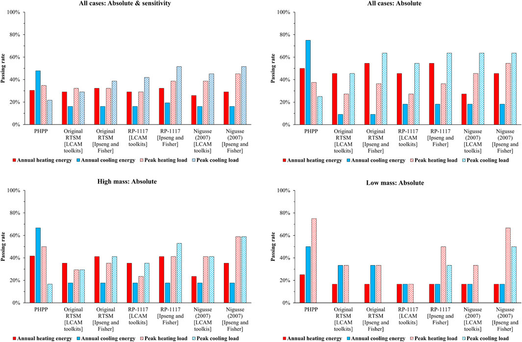
Figure 2. The passing rate of the PHPP and RTSM, in percentage, of (starting from top left): 1) all cases, absolute and sensitivity; 2) all cases, absolute; 3) high mass, absolute; and 4) low mass, absolute.
For the annual heating energy (absolute values) for the low mass cases, the Original RTSM [Ipseng and Fisher] and RP-1117 [Ipseng and Fisher] achieve the highest passing rate (both 55%), exceeding PHPP’s 50%. For the annual cooling energy, however, the PHPP’s passing rate (75%) far exceeds that of the RTSM’s methods (18% for both RP-1117 and Nigusse (2007)). It can be noted that the passing rate for annual cooling energy is doubled (from 9% to 18%) when a correction approach—either the RP-1117 or Nigusse (2007)—is applied to the Original RTSM, indicating that the intent of these correction approaches, at least in the low mass cases, has been achieved.
The situation differs when we look at the peak heating and cooling loads. For the heating load, Nigusse (2007) [Ipseng and Fisher] achieves the highest score (55%), whereas the PHPP is behind at 38%. Similarly, for the cooling load, all the RTSM approaches achieve a considerably higher score than PHPP’s 25%—e.g., 64% for the RP-1117 and Nigusse (2007) approaches. This puts into questions the claim of the validity of PHPP’s estimates of a building’s annual and peak heating demands, especially that of low mass buildings (Passipedia, 2022), given that its BESTEST passing rate was inferior to that of the RTSM.
For the high mass cases (the 900 series), the PHPP passes 25% of the cases for the annual heating energy (absolute value), exceeding that achieved by all the RTSM methods (17% for all cases). Similarly, for annual cooling, the PHPP has the highest passing rate (50%). Perhaps oddly, the Original RTSM achieves a higher score (33%) compared with the two correction approaches (17% for both)—putting into question whether the intent of the correction approaches has been achieved. For the peak heating load, the PHPP is within the range established by the BESTEST reference programmes for 75% of the cases, whereas the highest passing rate for the RTSM (67%) was achieved by Nigusse (2007) [Ipseng and Fisher]. For the peaking cooling load, Nigusse (2007) [Ipseng and Fisher] achieved the highest passing rate (50%)—far exceeding that of the PHPP (0%).
A comparison is carried out between the output of the PHPP and various RTSM methods, and that of the BESTEST reference programmes (shown in Table 1) and is displayed in Figure 3. For brevity, only the results of cases 600 and 930 are displayed, whilst the results for rest of the cases can be viewed in the paper’s Supplementary Data.
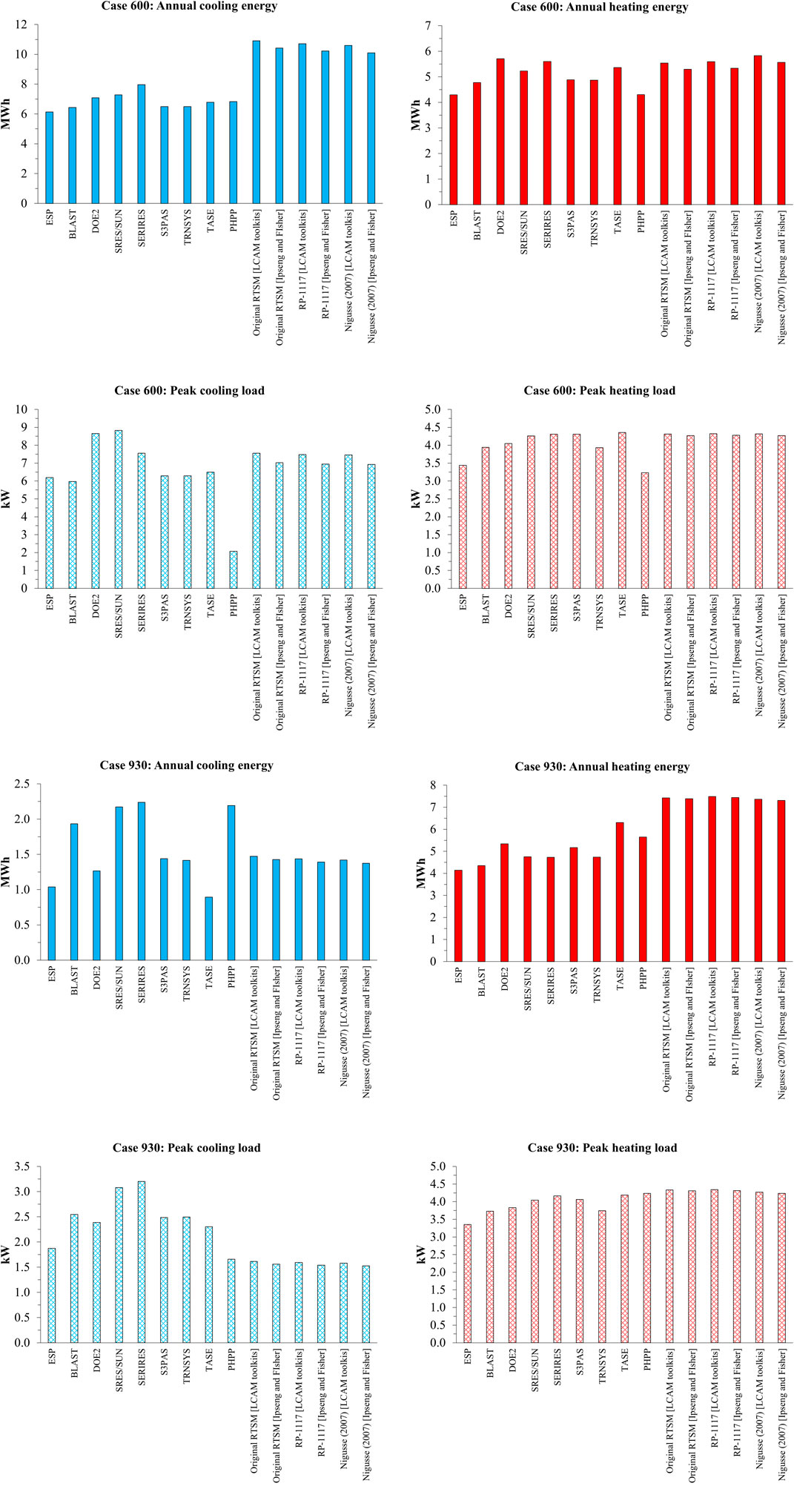
Figure 3. . Comparison between the output (absolute value) of the BESTEST reference programmes and that of PHPP and various RTSM correction approaches for Case 600 (top four) and Case 930 (bottom four) for the annual heating, annual cooling, peak heating, and peak cooling.
As can be noted, compared with the reference software, the PHPP generally underestimates the energy demand and peak loads for the low mass cases. Another general trend is that for the RTSM methodology, using the LCAM toolkits (Spitler, 2014) to compute the CTFs and RTFs leads to an overestimation of annual energy and peak loads compared with when the Ipseng and Fisher (2003) tool is used. Unlike what has been noted above, the tool chosen to compute the CTFs and RTFs seems to make more of a difference in both the cooling energy and peak load compared with the chosen correction approach (i.e., RP-1117 or Nigusse (2007)).
For the low mass Case 600, the PHPP provides a relatively low estimate for annual heating (though still within the BESTEST range) and the lowest estimate for peak heating and cooling which falls outside the range established by the BESTEST reference programmes. For the RTSM, with the exception of the annual cooling energy (which is considerably overestimated), its results fall within the BESTEST range under all approaches (i.e., Original, RP-1117, and Nigusse (2007)) and CTF and RTF estimation methods (LCAM toolkits and Ipseng and Fisher).
For the high mass Case 930, PHPP’s underestimation can be noted for peak cooling, whereas its results for the annual heating and cooling fall within the BESTEST range. For the RTSM, all the correction approaches pass the annual cooling energy but, for the peak cooling load, none of the RTSM approaches pass and an underestimation of 19% is noted for the (Nigusse (2007) [Ipseng and Fisher]) approach when compared with BESTEST’s lowest value (ESP). Similarly, none of the RTSM approaches pass the ranges established by the BESTST reference programmes for annual heating energy nor the peak heating load.
3.1 Comparison with other research
As mentioned in Section 1.2 and Section 1.3, neither the PHPP nor the RTSM have undergone testing in accordance with the BESTEST document that the majority of simulation programmes follow to validate their output (Judkoff and Neymark, 1995b). Therefore, it would not be possible to compare the outcome of these tools reported in this paper with that of other research. However, as the ISO 52016 hourly method (2017) has been (partially) tested in accordance with BESTEST, it might be somewhat useful to compare its outcome with PHPP, even as the latter is based on ISO 52016’s monthly method. It must be noted that only cases 600, 640, 900, and 940 were reported in the ISO standard, with no clear explanation given as to why the rest of the cases (i.e., 610, 620, 630, 650, 910, 920, 930, and 950) were not included. Due to PHPP’s inability to set specific heating and cooling set points at particular hours (as discussed in Section 2.1), the comparison that follows only includes cases 600 and 900.
As can be seen in Figure 4, the difference between ISO 52016 hourly method and the PHPP is more pronounced in the peak load estimations (where the former is higher by a maximum of 67%) compared with the annual energy estimations (where the former is higher by a maximum of 30%). This is with the exception of the annual cooling energy for Case 900, where PHPP’s estimate is 54 times higher than that of the hourly method6.
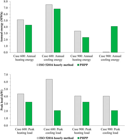
Figure 4. A comparison between ISO 52016’s hourly method and PHPP (as reported in this paper) for cases 600 and 900, for the annual heating and cooling energy (top) and peak heating and cooling loads (bottom).
As a side note, in the BESTEST results reported in the ISO 52016 standard, the output of ISO’s hourly method falls within the range established by BESTEST except for the annual heating and cooling energy of Case 900 and the annual cooling energy of Case 940 (both high mass). Additionally, the selected test cases (600, 640, 900, and 940) do not test the standard’s ability to predict the effects of south overhangs, east and west overhangs and fins, and solar transmittance. The sensitivity tests—i.e., the difference between the results of various cases which are used to assess a tool’s sensitivity to certain changes—were also not included. All this subtly suggests that further calibration of the standard might be needed and also somewhat contradicts van Dijk (2016) in that ISO 52016s hourly method “has been successfully validated using [BESTEST]”.
In any case, it could be postulated from this comparison that, had the PHPP implemented ISO 52016s hourly method rather than its monthly method, then its underestimation of peak heating and cooling loads reported in Section 3 could have been minimised and thus a higher passing rate might have been achieved. To an extent, this is in-line with the suggestion made by van Dijk (2018) where ISO 52016s hourly method was preferred over its monthly method.
Although explaining the differences between ISO 52016 hourly method and PHPP falls outside the scope of this paper, it is useful to examine what this difference could be due to. One factor could be the dirt factor that the PHPP assumes and which, to the best of the author’s knowledge, could not be altered in the PHPP spreadsheet. As this means that comparatively less solar irradiation would penetrate into the space, this could partially explain PHPP’s peak cooling load being lower than that of ISO’s hourly method for both cases.
Another difference which likely stems from PHPP’s reliance on ISO 52016s monthly method, is that the PHPP calculates the cooling load based on daily average weather conditions (Sarah, 2017), whereas the hourly method is able to take into account the weather’s hourly fluctuations.
Notably, as stated under Section 2.1, PHPP’s formulae was altered for the dirt factor, the internal heat gains, and infiltration rate such that it yields values that match those required under BESTEST. The full results of this ‘modified’ PHPP version are presented in the paper’s Supplementary Data, but it suffices to note here that the overall passing rate of this version is 28%—lower than that of the official PHPP version (34%) reported under Section 3. An important caveat here is that due to the complexity of the PHPP, it is possible that altering one or more of its formulae could results in inconsistencies in its internal algorithm. Thus, the results of this modified PHPP version could have been affected by some of these inconsistencies.
4 Conclusion
Current research shows that, to align the buildings sector with the 1.5°C climate change trajectory, enormous improvements in energy efficiency—far greater than ever achieved—are needed. It is therefore crucial that the tools we use to assess the effect of energy efficiency measures are robust and tested following state-of-the-art verification procedures. The paper shows that, to date, the most robust methodology available for comparatively testing building simulation tools is the Building Energy Simulation Test (BESTEST) developed by the National Renewable Energy Laboratory (NREL), which later formed the basis for ASHRAE Standard 140. Based on BESTEST, this paper tests, for the first time, the validity of both the Passive House Planning Package (PHPP) and an author-modified version of the Radiant Time Series Method (RTSM), for both their annual and peak heating and cooling demand estimates. The modification introduced to the RTSM tool enabled a quasi-steady state periodic conditions algorithm, as opposed to the original RTSM’s steady periodic conditions assumption, and allows the tool to read hourly weather data from a TMY weather file. The results reported for the RTSM in this paper include the two correction approaches (RP-1117 and Nigusse (2007)) that were developed with the intent to minimise the original RTSM’s overestimation of cooling loads. This exercise also includes (and tests) the two methods used to estimate the Conduction Time Factors (CTFs) and Radiant Time Factors (RTFs) of the RTSM—i.e., the LCAM’s toolkits and the Ipseng and Fisher’s tool.
The results show that, when modified, the validity of the RTSM slightly exceeds that of the PHPP, for both energy demand and peak load calculations. This shows that, contrary to the recommendation made by ASHRAE in that the RTSM should only be used for peak load estimation, the modified RTSM is capable of producing energy and load estimations that are superior in their validity to those produced by the PHPP.
A general trend that was noted is that the PHPP, when compared with the BESTEST tools, tends to underestimate the energy demand and peak loads for the low mass cases. For the RTSM, applying the CTFs and RTFs computed using LCAM toolkits’ leads to higher energy demand and peak load estimates compared to when those derived from the Ipseng and Fisher tool are applied. Additionally, it cannot be definitively said which RTSM correction approach is the most robust given that the three approaches tend to achieve the highest scores in different cases. However, overall, both the Nigusse (2007) [Ipseng and Fisher] and the Original RTSM [Ipseng and Fisher] tend to pass the highest number of BESTEST cases. Notably, the paper highlights that the intent of both RTSM’s correction approaches—i.e., RP-1117 and Nigusse (2007)—in reducing the peak cooling has not been clearly demonstrated, and that the choice of CTFs and RTFs computation tool (i.e., the LCAM’s toolkit or the Ipseng and Fisher’s tool) has a more pronounced effect in that regard.
Towards the end, a comparison between the PHPP’s BESTEST outcome reported in this paper and that of ISO 52016’s hourly method was conducted. The results showed that while the two tools produce similar results for the heating and cooling energy demand, their results differed considerably when estimating peak loads. This could be due to, the paper postulates, the PHPP setting shading and dirt factors for windows—that cannot be altered—and which would limit the amount of solar irradiation entering a space. Another reason that was noted is that the PHPP calculates the cooling load based on daily average weather conditions, whereas ISO 52016’s hourly method is able to take into account weather’s hourly fluctuations.
In summary, neither the PHPP nor the RTSM (in all its variations) were able to pass more than 35% of all the BESTEST cases. This brings into question the widely-held belief of PHPP being ‘validated’ for both its annual heating energy and peak heating load estimates given that they only fall within the BESTEST range for 42% and 50% of the tested cases, respectively. Also, as the modified RTSM only passes a maximum of 59% of the cases for peak heating and cooling load estimations, the validity of its intended purpose as presented by ASHRAE (Spitler, 2014) is somewhat questionable.
As explained in Section 1.1, while this does not necessarily invalidate the outcome of these tools, it does indicate that they are in need of further calibration. For the PHPP, the criticality of this lies in that it is the only tool that can be used to demonstrate compliance with the Passivhaus standard—a standard that has more than 5,000 certified buildings worldwide and has been gaining momentum in the past few years (Boston Business Journal, 2022; International Passive House Association, 2023; Passivhaus Trust UK, 2024b). This also has important implications for policymakers, especially in provinces that have adopted the Passivhaus standard, as it shows that the energy savings that these provinces sought to achieve through that adoption might not be fully realised. Notably, from the comparison conducted between PHPP and ISO 52016’s hourly method, it could be postulated that, had the PHPP implemented ISO 52016’s hourly method rather than its monthly method, then its underestimation of peak loads could have been minimised and thus a higher passing rate under BESTEST might have been achieved.
For the RTSM, given its adoption by both engineering programmes and design professionals for estimating peak heating and cooling loads (as discussed in Section 1.3), the findings of the paper point to the urgent need for calibrating the RTSM in order to avoid incorrect sizing of HVAC equipment which, consequently, would increase the energy demand of buildings. Nonetheless, the paper demonstrates that the RTSM—when modified—has the potential to be an energy-estimation tool in addition to a load-estimation tool, given that its BESTEST passing rate is comparable to that of PHPP.
The limitations of the paper include the possibility of human error when inputting the parameters of the BESTEST cases into the PHPP and modified RTSM tools. While the inputs were checked several times, the possibility of an error still remains. Another limitation concerns the Meteonorm tool that was used to export the BESTEST’s TMY weather file into a PHPP format. This relates to how representative that exported file is of the original TMY file, especially given the considerable impact that climate data can have on the outcome of energy simulations (as demonstrated in Section 1). Related to this is the way in which the Passive House Institute computes the peak loads of a certain location, which is usually done through a reverse-engineering exercise involving multi-stage dynamic simulations (McLeod et al., 2012). Thus, the peak loads determined through the Meteonorm tool may not perfectly match with those that would be determined by the Passive House Institute for the BESTEST weather file.
Related to this is the internal heat gain input in the PHPP for cases where BESTEST stipulates an internal heat gain of zero (i.e., cases 400 and 410). Inserting “0” as the value for internal heat gains in PHPP’s IHG sheet flags an error, and thus it is possible that the annual energy and peak loads for heating and cooling computed by the PHPP for these two cases are flawed as a result of that error. In this context, it is also important to note that the specific heat capacity values stipulated by BESTEST (15.81 and 89.58 Wh/K•m2 for the lightweight and heavyweight constructions, respectively, as determined in Table 2) are considerably less than those recommended by the Passive House Institute (i.e., 60 and 204 Wh/K•m2, respectively).
As both the PHPP and RTSM present a relatively simple and cost-effective way of assessing the impact of various energy efficiency measures, their advantages over fully dynamic and resource-intensive simulation programmes are clear. Therefore, to fully utilise that advantage, future research could look into optimising their underlying methodologies such that their outcome compares well with the BESTEST reference programmes.
Data availability statement
The original contributions presented in the study are included in the article’s Supplementary Material. Further inquiries can be directed to the corresponding author.
Author contributions
BAS: Conceptualization, Data curation, Formal Analysis, Investigation, Methodology, Software, Validation, Visualization, Writing–original draft, Writing–review and editing.
Funding
The author declares that financial support was received for the research, authorship, and publication of this article. The PhD research project upon which this paper is based was supported by a doctoral studentship under the Engineering and Physical Sciences Research Council (EPSRC) “Centre for Decarbonisation of the Built Environment (dCarb)” [grant ref EP/L016869/1], and the Royal Academy of Engineering funded “Preparing the South African Built Environment for Climate Change Resilience (SABER)” project [grant ref IAPP1617\59].
Acknowledgments
I would like to thank the two peer reviewers for taking the time to review the manuscript. The comments and suggestions of Reviewer 1 were especially helpful, and have made the paper more robust, and the methodologies implemented more scientifically-sound.
I wish to thank Tristan Kershaw and Sukumar Natarajan for their comments on the PhD thesis upon which this paper is based.
Conflict of interest
Author BAS was employed by Joule Consulting Group.
Publisher’s note
All claims expressed in this article are solely those of the authors and do not necessarily represent those of their affiliated organizations, or those of the publisher, the editors and the reviewers. Any product that may be evaluated in this article, or claim that may be made by its manufacturer, is not guaranteed or endorsed by the publisher.
Supplementary material
The Supplementary Material for this article can be found online at: https://www.frontiersin.org/articles/10.3389/fbuil.2024.1426774/full#supplementary-material
Abbreviations
ASHRAE, American Society of Heating, Refrigerating, and Air-conditioning Engineers; BESTEST, Building Energy Simulation Test; BIM, Building Information Modelling; CEPHEUS, Cost Efficient Passive Houses as European Standards; CERL, Civil Engineering Research Laboratory; CLTD, Cooling Load Temperature Difference; CTF, Conduction Time Factor; EPW, EnergyPlus Weather file; HBM, Heat Balance Method; HERS, Home Energy Rating System; HVAC, Heating, Ventilation, and Air Conditioning; IEA, International Energy Agency; ISO, International Organisation for Standardisation; LCAM, Load Calculation Applications Manual; NREL, National Renewable Energy Laboratory; PHPP, Passive House Planning Package; RP, ASHRAE Research Project; RTF, Radiant Time Factor; RTSM, Radiant Time Series Method; SEL, Solar Energy Laboratory; SHC, Solar Heating and Cooling; TFM, Transfer Function Method; TMY, Typical Meteorological Year UNITS; ACH, Air changes per hour; J, Joule; K, Kelvin; kg, kilogram; kW, kilowatt; m, metre; MWh, Megawatt-hour.
Footnotes
1It is important to note that Mao (2016) has attempted to reproduce the results of ASHRAE’s RP-1117 modified approach using the ASHRAE Loads Toolkit (Spitler, 2014), but the cooling loads obtained were lower than those stated in the RP-1117 report.
2It is not clear from ASHRAE’s report whether Nigusse’s (2007) Approach II or Approach III was used (Spitler and Nigusse, 2010). A comparison between the two was performed by the author and their outcome tested against BESTEST, with Approach III yielding relatively better results. Therefore, Approach III was used in this paper.
3This is unlike the ASHRAE 140 Class II tests where a 93% confidence interval is recommended (2017).
4The mistakes relate to numerical errors in the example on page 18.44.
5As the author has followed version 2017 of the standard, it may be the case that these mistakes were corrected in the newer (2021) version.
6It is likely that this value (occurring in Table 29, p. 131 of the ISO 52016, part 1 (ISO, 2017)) is a typo. The author has contacted the British Standards Institution (BSI) regarding this, but no response was received to date.
References
Al Shawa, B. (2022). The ability of Building Stock Energy Models (BSEMs) to facilitate the sector’s climate change target in the face of socioeconomic uncertainties: a review. Energy Build. 254, 111634. doi:10.1016/j.enbuild.2021.111634
Asdrubali, F., D’Alessandro, F., Baldinelli, G., and Bianchi, F. (2014). Evaluating in situ thermal transmittance of green buildings masonries—a case study. Case Stud. Constr. Mater. 1, 53–59. doi:10.1016/j.cscm.2014.04.004
ASHRAE (2013). Supplemental files for load calculation applications manual. Second Edition. ASHRAE. Available at: https://www.ashrae.org/technical-resources/bookstore/load-calculation-applications-manual (Accessed September 2, 2018).
ASHRAE Standard 140-2011 (2011). Standard method of test for the evaluation of building energy analysis computer programs.
ASHRAE Standard 140-2017 (2017). Standard method of test for the evaluation of building energy analysis computer programs.
Bhandari, M., Shrestha, S., and New, J. (2012). Evaluation of weather datasets for building energy simulation. Energy Build. 49, 109–118. doi:10.1016/j.enbuild.2012.01.033
Boston Business Journal (2022). Passive House standards are gaining momentum in Boston’s CRE industry. Boston Business Journal. Available at: https://www.bizjournals.com/boston/news/2022/01/19/passive-house-standards-are-gaining-momentum.html (Accessed August 19, 2023).
builddesk (2023). Heat capacity (Kappa value k) and thermal mass [WWW Document]. builddesk. Available at: https://builddesk.co.uk/software/builddesk-u/thermal-mass/(Accessed August 2, 2023).
Charron, R. (2019). PHPP v9.6 validation using ANSI/ASHRAE Standard. Remi Charron Consulting Services, 140–2017.
Chiu, F., and Krarti, M. (2021). Impacts of air-conditioning equipment sizing on energy performance of US office buildings. ASME J. Eng. Sustain. Build. Cities 2, 021001. doi:10.1115/1.4050937
Corrado, V., and Fabrizio, E. (2019). “Steady-state and dynamic codes, critical review, advantages and disadvantages, accuracy, and reliability,” in Handbook of energy efficiency in buildings (Elsevier), 263–294. doi:10.1016/B978-0-12-812817-6.00011-5
Crawley, D. B., Hand, J. W., Kummert, M., and Griffith, B. T. (2008). Contrasting the capabilities of building energy performance simulation programs. Build. Environ. 43, 661–673. doi:10.1016/j.buildenv.2006.10.027
DesignBuilder (2019). ANSI/ASHRAE Standard 14-2017: building thermal envelope and fabric load tests. Des. v61. EnergyPlus v8.9.
EDSL Tas (2024). Validation [WWW document]. Available at: https://www.edsltas.com/validation/ (Accessed March 17, 2024).
Feist, W., Peper, S., Gorg, M., and Hannover, S. (2001). CEPHEUS project information number 36. enercity.
Fisher, D., and Spitler, J. D. (2002). ASHRAE research project report RP-1117: experimental validation of heat balance/RTS cooling load calculation procedure. ASHRAE.
Florida Solar Energy Center (2012). ASHRAE standard 140-2007 standard method of test for the evaluation of building energy analysis computer programs: test results for the DOE-2.1e (v120) incorporated in EnergyGauge summit 4.0.
Henninger, R. H., and Witte, M. J. (2010). EnergyPlus testing with building thermal envelope and fabric load tests from ANSI/ASHRAE standard 140-2011 58.
Herrando, M., Cambra, D., Navarro, M., De La Cruz, L., Millán, G., and Zabalza, I. (2016). Energy Performance Certification of Faculty Buildings in Spain: the gap between estimated and real energy consumption. Energy Convers. Manag. 125, 141–153. doi:10.1016/j.enconman.2016.04.037
IEA (2022a) “Buildings: sectorial overview,”. IEA. Available at: https://www.iea.org/reports/buildings (Accessed June 21, 2023).
IEA (2022b) “Evolution of global floor area and buildings energy intensity in the Net Zero Scenario,”. IEA, 2010–2030. Available at: https://www.iea.org/data-and-statistics/charts/evolution-of-global-floor-area-and-buildings-energy-intensity-in-the-net-zero-scenario-2010-2030 (Accessed July 15, 2023).
IES (2018). Building envelope nd fabric load tests performance on ApacheSim in accordance with ANSI/ASHRAE Standard, 140–2014.
International Passive House Association (2023). iPHA: the global Passive House platform [WWW Document]. International Passive House Association. Available at: https://passivehouse-international.org/index.php?page_id=65 (Accessed August 22, 2023).
International Passive House Association (2024). Passive House legislation and funding [WWW document]. International Passive House Association. Available at: https://passivehouse-international.org/index.php?page_id=501 (Accessed March 18, 2024).
ISO (2008). Energy performance of buildings - calculation of energy use for space heating and cooling. ISO 13790:2008).
ISO (2017). ISO 52016-1:2017. Energy performance of buildings — energy needs for heating and cooling, internal temperatures and sensible and latent heat loads.
Johnston, D., Miles-Shenton, D., and Farmer, D. (2015). Quantifying the domestic building fabric performance gap. Build. Serv. Eng. Res. Technol. 36, 614–627. doi:10.1177/0143624415570344
Judkoff, R., and Neymark, J. (1995a). International Energy Agency building energy simulation test (BESTEST) and diagnostic method. No. NREL/TP--472-6231, 90674). doi:10.2172/90674
Judkoff, R., and Neymark, J. (1995b). International Energy Agency building energy simulation test (BESTEST) and diagnostic method: Supporting Files. No. NREL/TP--472-6231, 90674). doi:10.2172/90674
Judkoff, R., and Neymark, J. (2013). “Twenty years on!: updating the IEA BESTEST building thermal fabric test cases for ASHRAE standard 140,” in Presented at the building simulation conference (Chambery, France: National Renewable Energy Laboratory).
Kim, Y.-J., Yoon, S.-H., and Park, C.-S. (2013). Stochastic comparison between simplified energy calculation and dynamic simulation. Energy Build. 64, 332–342. doi:10.1016/j.enbuild.2013.05.026
Kokogiannakis, G., Strachan, P., and Clarke, J. (2008). Comparison of the simplified methods of the ISO 13790 standard and detailed modelling programs in a regulatory context. J. Build. Perform. Simul. 1, 209–219. doi:10.1080/19401490802509388
Mao, C. (2016). Analysis of building peak load calculation methods for commercial buildings in the United States. Texas A&M University.
McLeod, R. S., Hopfe, C. J., and Rezgui, Y. (2012). A proposed method for generating high resolution current and future climate data for Passivhaus design. Energy Build. 55, 481–493. doi:10.1016/j.enbuild.2012.08.045
Meteonorm (2024). Meteonorm software [WWW document]. Meteonorm. Available at: https://meteonorm.com/en/ (Accessed August 23, 2023).
Mitalas, G. P. (1972). Transfer Function Method of calculating cooling loads, heat extraction and space temperature. ASHRAE J. 14.
Mitchell, R., and Natarajan, S. (2020). UK Passivhaus and the energy performance gap. Energy Build. 224, 110240. doi:10.1016/j.enbuild.2020.110240
Nigusse, B. A. (2007). Improvements to the radiant time series method cooling load calculation procedure.
Passipedia (2022). Insulation vs. thermal mass [WWW Document]. Passipedia. Available at: https://passipedia.org/planning/thermal_protection/thermal_protection_works/thermal_protection_vs._thermal_storage (Accessed March 19, 2024).
Passipedia (2023). PHPP - validated and proven in practice [WWW Document]. Passipedia. Available at: https://passipedia.org/planning/calculating_energy_efficiency/phpp_-_the_passive_house_planning_package/phpp_-_validated_and_proven_in_practice (Accessed July 24, 2023).
Passive House Institute (2019a). Passive House institute/about us [WWW document]. Passive House Institute. Available at: https://passivehouse.com/01_passivehouseinstitute/01_passivehouseinstitute.htm (Accessed April 26, 2019).
Passive House Institute (2021). PHPP 10 [WWW document]. Passive House Institute. Available at: https://passivehouse.com/05_service/01_literature_online-order/00_literature-links/02_phpp.htm (Accessed August 1, 2023).
Passivhaus Trust, U. K., 2024b. Passivhaus benefits gain mainstream attention [WWW Document]. Passivhaus Trust UK. Available at: https://passivhaustrust.org.uk/news/detail/?nId=284 (Accessed August.19.2023).
Passivhaus Trust UK (2024a). Design support and PHPP tools [WWW document]. Passivhaus Trust UK. Available at: https://www.passivhaustrust.org.uk/design_support.php#:∼:text=The%20Passivhaus%20Planning%20Package%20(PHPP,assurance%20provided%20by%20the%20Standard (Accessed August 17, 2023).
Rittelmann, P. R., and Ahmed, S. F. (1985). Design tool survey (No. T.8.C.1.A), Solar heating and cooling - Task 8. International Energy Agency.
Ron, J., and Neymark, J. (1995). Home energy rating system BUilding energy simulation test (HERS BESTEST).
Salehi, M. M., Cavka, B. T., Fedoruk, L., Frisque, A., Whitehead, D., and Bushe, W. K. (2013). “Improving the performance of a whole-building energy modeling tool by using post-occupancy measured data,” in 13th conference of international building performance simulation association (Chambery, France), 1683–1689.
Sandberg, J. (2011). Computer based tools in the HVAC design process. Sweden: Chalmers University of Technology.
Saunders, H. (1992). The khazzoom-brookes postulate and neoclassical growth. Energy J. 13, 131–148. doi:10.5547/issn0195-6574-ej-vol13-no4-7
6sense (2024). Market share of Revit MEP [WWW document]. 6sense. Available at: https://6sense.com/tech/bim-and-architectural-design-software/revit-mep-market-share (Accessed March 18, 2024).
Shi, X., Si, B., Zhao, J., Tian, Z., Wang, C., Jin, X., et al. (2019). Magnitude, causes, and solutions of the performance gap of buildings: a review. Sustainability 11, 937. doi:10.3390/su11030937
Spitler, J. D. (2014). “Chapter 7: Fundamentals of the radiant time series method,” in Load calculation Applications manual. SI Edition (Atlanta, GA: ASHRAE).
Spitler, J. D., Fisher, D. E., and Pedersen, C. O. (1997). The radiant time series cooling load calculaton procedure. ASHRAE Trans. 103, 503–515.
Spitler, J. D., McQuiston, F. C., and Lindsey, K. L. (1993). The CLTD/SCL/CLF cooling load calculation method. ASHRAE Trans. 99, 183–192.
Spitler, J. D., and Nigusse, B. A. (2010). “Refinements and improvements to the radiant time series method (No. RP-1326),” in ASHRAE Transactions (ASHRAE).
Strachan, P. A., Kokogiannakis, G., and Macdonald, I. A. (2008). History and development of validation with the ESP-r simulation program. Build. Environ. 43, 601–609. doi:10.1016/j.buildenv.2006.06.025
Trucano, T. G., Swiler, L. P., Igusa, T., Oberkampf, W. L., and Pilch, M. (2006). Calibration, validation, and sensitivity analysis: what’s what. Reliab. Eng. Syst. Saf. 91, 1331–1357. doi:10.1016/j.ress.2005.11.031
van Dijk, D., Spiekman, M., and Hoe-van Oeffelen, L. (2016). EPB standard EN ISO 52016: calculation of the building’s energy needs for heating and cooling, internal temperatures and heating cooling load. REHVA J. 53, 18–22.
Keywords: building energy simulation, verification and validation, comparative test, BESTEST validation procedure, Passive House Planning Package (PHPP), Radiant Time Series Method (RTSM)
Citation: Al Shawa B (2024) Assessing the validity of simplified heating and cooling demand calculation methods: The case of Passive House Planning Package (PHPP) and Radiant Time Series Method (RTSM). Front. Built Environ. 10:1426774. doi: 10.3389/fbuil.2024.1426774
Received: 02 May 2024; Accepted: 24 June 2024;
Published: 12 August 2024.
Edited by:
Amirhossein Balali, The University of Manchester, United KingdomReviewed by:
Anton Dobrevski, Passive House School, BulgariaHasim Altan, Prince Mohammad bin Fahd University, Saudi Arabia
Copyright © 2024 Al Shawa. This is an open-access article distributed under the terms of the Creative Commons Attribution License (CC BY). The use, distribution or reproduction in other forums is permitted, provided the original author(s) and the copyright owner(s) are credited and that the original publication in this journal is cited, in accordance with accepted academic practice. No use, distribution or reproduction is permitted which does not comply with these terms.
*Correspondence: Bashar Al Shawa, Yi5hbHNoYXdhQGpvdWxlY29uc3VsdGluZ2dyb3VwLmNvbQ==