Predictive modeling of rocking-induced settlement in shallow foundations using ensemble machine learning and neural networks

Introduction: The objective of this study is to develop predictive models for rocking-induced permanent settlement in shallow foundations during earthquake loading using stacking, bagging and boosting ensemble machine learning (ML) and artificial neural network (ANN) models.

Methods: The ML models are developed using supervised learning technique and results obtained from rocking foundation experiments conducted on shaking tables and centrifuges. The overall performance of ML models are evaluated using k-fold cross validation tests and mean absolute percentage error (MAPE) and mean absolute error (MAE) in their predictions.

Results: The performances of all six nonlinear ML models developed in this study are relatively consistent in terms of prediction accuracy with their average MAPE varying between 0.64 and 0.86 in final k-fold cross validation tests.

Discussion: The overall average MAE in predictions of all nonlinear ML models are smaller than 0.006, implying that the ML models developed in this study have the potential to predict permanent settlement of rocking foundations with reasonable accuracy in practical applications.

1 Introduction

Structural fuse mechanisms, active and passive energy dissipation devices, and base isolation techniques have generally been used to improve the seismic performance of important structures (e.g., Soong and Spencer, 2002; Symans et al., 2008). Geotechnical seismic isolation, using various techniques, is a relatively new area of research that has been studied to some extent in the recent past. As such, the findings of recent experimental research on rocking shallow foundations reveal that rocking mechanism dissipates seismic energy in soil, reduces seismic demands imposed on structures, and can be used as geotechnical seismic isolation mechanism to improve the overall seismic performance of structures they support (e.g., Gajan et al., 2005; Paolucci et al., 2008; Anastasopoulos et al., 2010; Loli et al., 2014; Ko et al., 2019; Hakhamaneshi et al., 2020; Arabpanahan et al., 2023; Irani et al., 2023). In addition, it has been shown that appropriately-designed rocking shallow foundations can be as effective as structural energy dissipating mechanisms in terms of reducing the seismic demands experienced by key structural members (Gajan and Saravanathiiban, 2011; Gajan and Godagama, 2019). However, the material nonlinearities (yielding of soil and resulting plastic deformations), the geometrical nonlinearities associated with the soil-foundation system (partial separation of footing from supporting soil), and the uncertainties in soil properties and earthquake loading parameters pose significant challenges to the accurate prediction of permanent deformations in foundation during rocking.

A recent article reviews the commonly used numerical methods for modeling dynamic soil-structure interaction in shallow foundations during earthquake loading including spring-based Winkler foundation models, macro-element models for soil-foundation system, and continuum-based models (Bapir et al., 2023). Researchers in the past have developed constitutive models that relate the cyclic forces and displacements acting on the foundation during seismic loading and performed numerical simulations of rocking foundations incorporating nonlinear dynamic soil-foundation interaction (e.g., Allotey and Naggar, 2003; Gajan and Kutter, 2009; Gajan et al., 2010; Chatzigogos et al., 2011; Figini et al., 2012; Pelekis et al., 2021). Though the mechanics-based constitutive models and numerical simulation approaches for rocking foundations have sound theoretical basis, they include assumptions and simplifications in their formulations. Machine learning (ML) models, on the other hand, have the ability to generalize experimental behavior when they are trained and tested on data and results that cover a wide range of experiments conducted independently by different researches and using different types of equipment. Although the ML models can have their drawbacks (for example, they may not be able to capture every physical mechanism that governs the problem), they are capable of capturing the hidden complex relationships in data and have the potential to be used in addition to mechanics-based numerical models in practical applications.

As the number of widely available experimental databases increases, the use of ML techniques to model geotechnical engineering problems increases exponentially, especially in last 30 years (Ebid, 2021). For example, support vector machines, decision trees, and neural networks have been used in geotechnical engineering applications such as compaction characteristics of soils, mechanical properties and strength of soils, foundation engineering, soil slope stability, and geotechnical earthquake engineering (e.g., Goh and Goh, 2007; Mozumder and Laskar, 2015; Pham et al., 2017; Jeremiah et al., 2021; Amjad et al., 2022). Artificial neural networks, gene expression programming, and neuro-swam system algorithms have been used successfully for the prediction of settlement of shallow and deep foundations (Armaghani et al., 2018; Armaghani et al., 2020; Diaz et al., 2018). Recently, ML-based predictive models have been developed for normalized seismic energy dissipation, peak rotation, and acceleration amplification ratio of rocking foundations during earthquake loading (Gajan, 2021; Gajan, 2022; Gajan, 2023). A recent review article summarizes the recent advances in application of machine learning and deep learning tools to predict the properties of cementitious composites (concrete and fiber-reinforce concrete) at elevated temperatures (Alkayem et al., 2024). In addition to ML models alone, theory-guided ML is also becoming popular slowly in predictive modeling in engineering (Karpatne et al., 2017) and in geotechnical engineering in particular (Xiong et al., 2023).

2 Research significance and objective

Empirical relationships have been proposed for the estimation of permanent settlement of rocking shallow foundations using either the static vertical factor of safety (FS_v) or critical contact area ratio (A/A_c) of foundation and the cumulative rotation experienced by the foundation during earthquake loading (Deng et al., 2012; Hamidpour et al., 2022). A/A_c is conceptually a factor of safety for rocking foundations taking into account the change of contact area of the footing with the soil during rocking (Gajan and Kutter, 2008). The cumulative rotation (θ_cum) of the foundation is defined based on the instantaneous peak rotations experienced by the foundation (local maximums) that exceed a threshold value (Deng et al., 2012). The threshold value for this peak rotation is defined arbitrarily as 0.001 rad, assuming that rotations smaller than 0.001 rad do not cause permanent settlement. One difficulty or drawback of the cumulative rotation approach for the estimation of permanent settlement is that the θ_cum of the foundation can only be known after the earthquake shaking is over (i.e., θ_cum itself is a performance parameter of rocking foundation, and cannot be known before the earthquake to predict the rocking induced settlement of foundation).

The objective of this study is to develop predictive models for rocking-induced permanent settlement in shallow foundations during earthquake loading using stacking, bagging and boosting ensemble ML models and artificial neural network (ANN) model. Support vector regression (SVR), k-nearest neighbors regression (KNN), stacked generalization (Stacking), random forest regression (RFR), adaptive boosting regression (ABR), and fully-connected artificial neural network regression (ANN) algorithms have been utilized in this study. The ML models are trained and tested using results obtained from rocking foundation experiments conducted on shaking tables and centrifuges. Critical contact area ratio of foundation, slenderness ratio of structure, rocking coefficient of rocking soil-foundation-structure system, peak ground acceleration of earthquake, Arias intensity of earthquake ground motion, and a binary feature for type of soil have been used as input features to ML models. The significance of the study presented in this paper is that this is the first time data-driven predictive models are developed for rocking-induced settlement of shallow foundations using ML and deep learning algorithms. In addition, the input features used are in the form of normalized, non-dimensional soil-foundation system parameters and earthquake ground motion parameters that are readily available for design of structures in majority of the seismic zones.

3 Rocking-induced settlement in shallow foundations

3.1 Settlement-rotation relationship

Figure 1A illustrates the schematic of a rocking structure-foundation system and the forces and displacements acting on the foundation during earthquake loading. For rocking on a 2-D plane, these forces and displacements include vertical load (V), settlement (s), shear force (H), sliding (u), moment (M), and rotation (θ). Figures 1B, C present experimental results for cyclic settlement versus rotation response at the base center point of foundation supported by sandy soils. Note that the settlement is normalized by the width of the footing (NS = s/B). Figure 1B presents the results obtained from a centrifuge experiment (FS_v = 4 and a_max = 0.55 g) (Gajan and Kutter, 2008), while Figure 1C presents the results obtained from a shaking table experiment (FS_v = 24 and a_max = 0.36 g) (Antonellis et al., 2015), where FS_v is the static factor of safety for bearing capacity failure and a_max is the peak ground acceleration of the earthquake.

Figure 1

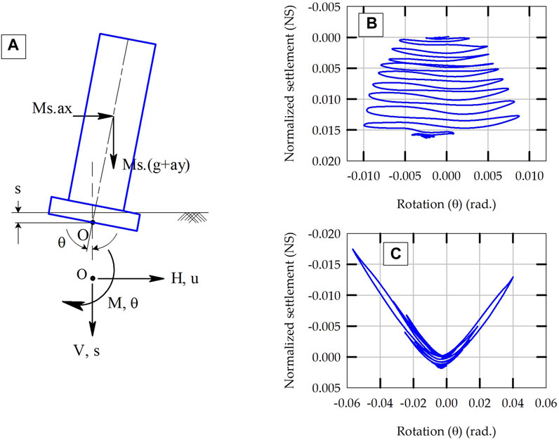
Figure 1. (A) Illustration of major forces and displacements acting on a rocking structure, and experimental results of settlement versus rotation response at the base of rocking foundations: (B) FS_v = 4 and a_max = 0.55 g and (C) FS_v = 24 and a_max = 0.36 g.

As shown in Figure 1B, the foundation keeps accumulating settlement as the seismic shaking progresses and as the footing rocks, with the permanent settlement being equal to about 1.6% of the width of the footing (NS = 0.016) at the end of shaking. For the other test (FS_v = 24, Figure 1C), as the footing rocks, a gap opens between the soil and the footing and it results in instantaneous uplift of the footing (the negative values on NS axes represent uplift of footing). Therefore, the settlement-rotation response shows smaller permanent settlement for higher FS_v foundations (NS = 0.00175). For relatively lower FS_v foundations, the settlement-rotation response is dominated by yielding of soil (material nonlinearity) whereas for higher FS_v foundations, it is dominated by uplift of footing (geometrical nonlinearity). The rocking-induced permanent settlement in shallow foundations depends primarily on FS_v and the magnitude, number of cycles, and duration of earthquake loading.

3.2 Experimental results and key parameters

The experimental data and results utilized in this study are extracted from a rocking foundations database (Gavras et al., 2020). This database is freely accessible and available in Design-Safe-CI website (https://doi.org/10.13019/3rqyd929) (Gavras et al., 2023). This database has results obtained from centrifuge and shaking table experiments on rocking foundations conducted by several researchers (Gajan and Kutter, 2008; Deng et al., 2012; Deng and Kutter, 2012; Drosos et al., 2012; Hakhamaneshi et al., 2012; Anastasopoulos et al., 2013; Antonellis et al., 2015; Tsatsis and Anastasopoulos, 2015). A summary of results of these experiments, in terms of rocking foundations performance parameters, is also available in the literature (Gajan et al., 2021).

Rocking coefficient (C_r) is essentially the normalized ultimate moment capacity of a rocking foundation and is given by (Deng et al., 2012),

$C_r=\frac{B}{2.h}.\left[1-\frac{A_c}{A}\right]$

where h is the effective height of the structure (height of center of gravity of the structure from the base of the footing). Arias intensity (I_a) of the ground motion is essentially the numerical integration of earthquake ground acceleration in time domain. The effects of number of cycles of earthquake loading, amplitude of cycles, frequency content and duration are combined in I_a, and it is defined as (Kramer, 1996),

$I_a=\frac{\pi }{2.g}{\displaystyle \underset{0}{\overset{t_{fin}}{\int }}}{\left[a\left(t\right)\right]}^{2}dt$

where a(t) is horizontal ground acceleration as a function of time (t), g is the gravitational acceleration, and t_fin is the duration of earthquake.

Figure 2 presents the results for experimentally measured normalized permanent settlement (NS) of rocking foundations obtained from 140 individual experiments. The results presented in Figure 2 are grouped based on the rocking coefficient (C_r) of foundation and type of soil. As both NS and I_a depend on the amplitude, number of cycles and duration of earthquake loading, the NS results are plotted as a function of I_a in Figure 2. For a given C_r range and soil type, NS seems to increase with I_a; however, the variability in data indicates the presence of the effects of other variables. Another observation is that the NS in clayey soil foundations are smaller than in sandy soil foundations with the same C_r range (C_r > 0.2). This is consistent with the findings of recently published results on rocking-induced settlement in shallow foundations supported by clayey soils during slow lateral cyclic loading (Sharma and Deng, 2019; Sharma and Deng, 2020). When the data presented in Figure 2 are divided into three groups (based on their C_r values and soil type) and are fit using a statistics-based simple linear regression model, they yield coefficients of determination (R²) values that are smaller than 0.35. This indicates that purely statistics-based models are not capable of capturing the permanent settlement of shallow foundations satisfactorily.

Figure 2

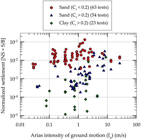
Figure 2. Experimental results of normalized settlement of rocking foundations used in the development of machine learning models.

3.3 Input features for machine learning models

In addition to the above-mentioned variables (C_r, I_a and type of soil), rocking induced settlement of foundations also depends on A/A_c, h/B, and peak ground acceleration of the earthquake (a_max). All of these six variables are chosen as the input features for the ML models developed in this study. The selection of input features is based on the experimentally observed relationships between NS and the input feature parameters found in previously published results (Gajan et al., 2021). The input feature selection is further justified in Section 5.2: Sensitivity of ML models to input features. Figure 3 plots the statistical distributions of five input features showing the variation (numerical range) of each of the input feature extracted from the experimental database. The box plots present the mean and median along with the 10th, 25th, 75th and 90th percentile values of each of the five input features used in the development of ML models. Table 1 summarizes the range of values, mean and coefficient of variation (COV) of all six input features and prediction parameter (NS). The type of soil is represented by a binary variable: 0 for sandy soil foundations and one for clayey soil foundations. As the variation of I_a and NS are relatively high (I_a varies from 0.03 m/s to 26.4 m/s, while the NS values are in the range of 10⁻⁵ to 10⁻¹), these two parameters are transformed to log-scale (base 10). In addition, all the input feature values are normalized in such a way that the values of each input feature vary between 0.0 and 1.0.

Figure 3

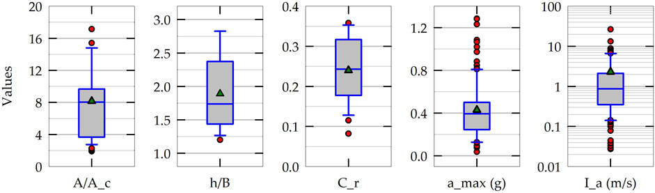
Figure 3. Statistical distributions (variations of experimental data) of five input feature parameters used in the development of machine learning models.

Table 1

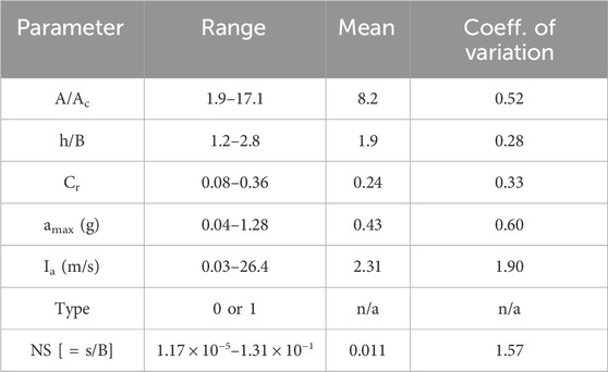
Table 1. Statistical distributions of input features and prediction parameter (normalized settlement, NS) used in this study.

4 Materials and methods

4.1 Base machine learning algorithms

Three base ML algorithms are considered in this study: k-nearest neighbors regression (KNN), support vector regression (SVR), and decision-tree regression (DTR). The KNN algorithms works by learning to predict the output based on the test data point’s nearest neighbors in training dataset (using the input feature values as distance measures), their output values, and their distance from the test data point. The number of neighbors to consider and the method of calculating the distance between two data points in a multi-dimensional input feature space are hyperparameters of the KNN model. The SVR algorithms makes the predictions by learning a hyperplane with a margin using training dataset in multi-dimensional space. The hyperparameters of SVR model include the margin of the hyperplane and a penalty parameter called C that determines the magnitude of tolerance used to adjust the margin (to accommodate datasets that have outliers). The DTR algorithms builds a tree-like data structure based on the input feature values and outputs of the training dataset and then makes predictions on test data using this tree. The maximum depth of the tree and the error criteria used to split the training data to build the tree (to create leaves) are the key hyperparameters of the DTR model.

4.2 Ensemble machine learning algorithms

Three ensemble ML algorithms are considered in this study: stacking, bagging, and boosting. Stacking model combines the predictions of multiple well-performing base ML models. In the process, the stacked model harnesses the best characteristics of the base models and makes predictions that are better than those of the base models. In this study, the predictions from KNN and SVR models are combined using linear regression as the meta model to create a stacking ensemble model. The training data for the stacked model consist of the outputs (predictions) of the base models and the actual, expected outputs. During testing, the stacked model combines the predictions of base models on test data using the trained linear regression meta model to make the prediction. The bagging and boosting ensemble techniques are implemented using random forest regression (RFR) and adaptive boosting regression (ABR), respectively. In both cases, multiple base DTR models are combined to create the ensemble model. The RFR model builds multiple individual trees (DTR models) of different depths and using random subsets of input features and then simply combines them together in such a way that the final prediction of the RFR model is the average value of each base DTR models in the ensemble. The ABR model also builds multiple DTR models, but sequentially, in such a way that the succeeding DTR models attempt to correct the error made by their preceding trees in the ensemble. The ABR model uses two sets of weights (data instance weights and predictor weights) and the final prediction of ABR model on test data is a weighted average value of the predictions of each base DTR models in the ensemble. The major hyperparameter of the RFR model include the number of trees in the ensemble and the maximum input features to consider when building an individual tree. The major hyperparameter of the ABR model include the number of trees in the ensemble and the learning rate of the model.

4.3 Artificial neural network model

Figure 4 schematically illustrates the architecture of the sequential, fully-connected, multi-layer perceptron artificial neural network (ANN) regression model considered in this study. While the number of neurons in the input layer (six, one for each input feature) and output layer (one for the prediction parameter, NS) are fixed, the number of hidden layers and the number of neurons in each hidden layer are varied systematically using hyperparameter turning and grid search to obtain their optimum values for the problem considered. The commonly used stochastic gradient descent (SGD) algorithm is used with the feed-forward, back-propagation algorithm to train the ANN models. As shown in Figure 4, the neurons in the input layer simply pass the input features to all the neurons in the first hidden layer. The outputs (y) of the neurons in the hidden layers are computed using the following relationship based on the inputs (X), network connection weights (W), bias parameters (b), and an activation function (g) (Geron, 2019; Deitel and Deitel, 2020).

$y_i=g\left({\sum }_{j=1}^k\left(W_{j,i}{X}_j\right)+b_i\right)$

Figure 4

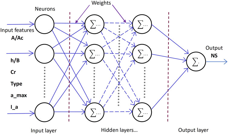
Figure 4. Schematic of the artificial neural network architecture utilized in this study.

The network is first trained using the training data and back-propagation algorithm and the optimum values for the network connection weights are found. When making a prediction on test data, the ANN model propagates the test data instance using forward-propagation and computes the output using the above equation with the optimum connection weights.

4.4 Flowchart of research methodology

Figure 5 presents the flowchart of the research methodology of this study. The experimental data is first randomly split into training dataset and testing dataset using a 70%–30% split. Results from a total of 140 experiments are considered in this study (Figure 2) and this split yields 98 training data instances and 42 testing instances. First, the ML models are trained using the training dataset and the hyperparameters of the ML models are tuned using k-fold cross validation tests considering training dataset only. The results of training error and hyperparameter turning presented in this paper are obtained from this phase of the research process. Second, the trained ML models with optimum values of hyperparameters are tested using the testing dataset and the results for testing error are obtained using this phase. Finally, to compare the overall performance of ML models, the ML models with the optimum hyperparameters are evaluated using k-fold cross validation tests considering entire dataset. For both k-fold cross validations, repeated 5-fold cross validation tests are carried out (with number of repeats being equal to 3). Mean absolute percentage error (MAPE) and mean absolute error (MAE) are used to evaluate the performance of ML models by comparing their predictions of NS with experimental results. MAE quantifies the error by averaging the absolute difference between predicted and actual (experimental) values for NS, while MAPE quantifies the average error by normalizing the absolute difference between predicted and actual values by the actual value of NS. It should be noted that a multivariate linear regression (MLR) ML model is also developed for the purpose of comparison of results and performance of all the ML models. All the ML models are implemented in Python programming platform using the functional classes available in Scikit-Learn (https://scikit-learn.org/stable/) and TensorFlow and Keras (https://keras.io/) libraries (Geron, 2019; Deitel and Deitel, 2020).

Figure 5

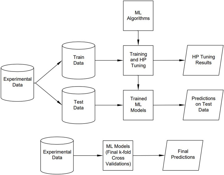
Figure 5. Flowchart of research methodology showing the sequence of key processes.

5 Results and discussion

5.1 Initial evaluation of base and ensemble machine learning models

Figure 6 presents the testing results of four base ML models: MLR, KNN, SVR and DTR. For all four models, the predicted results of NS are plotted on y-axes against the experimental results on x-axes along with 1:1 comparison lines. It should be noted that the hyperparameters of all the models are kept at their optimum values for these predictions (please see Section 5.3). The testing MAPE values, calculated using 48 testing data results, are also included in Figure 6 for all four models. As seen in the figure, the KNN model (MAPE = 0.48) performs better than the other models in terms of accuracy of predictions and it is followed by SVR model (MAPE = 0.51). The base DTR model (a single decision tree) shows poor performance (MAPE = 0.77) during testing phase, even worse than the baseline MLR model (MAPE = 0.70). Figure 7 presents the testing results of Stacking, RFR and ABR ensemble ML models. KNN and SVR models are combined using linear regression meta-model to build the Stacking model. Other combinations of stacking were also tested; however, their performance did not improve. For RFR and ABR models, 100 base DTR models are combined using bagging and boosting techniques, respectively. The prediction accuracy of RFR and ABR ensemble models on test data is improved significantly (MAPE = 0.45 and 0.53) when compared to a single DTR model (about 30%–40% improvement in prediction accuracy). From the results presented in Figure 7, it appears that the Stacking model is not effective (MAPE of Stack model is 0.5 whereas the MAPE of KNN alone is 0.48). However, in final k-fold cross validation tests of models (presented in Section 5.7), the effectiveness of Stacking model becomes apparent.

Figure 6

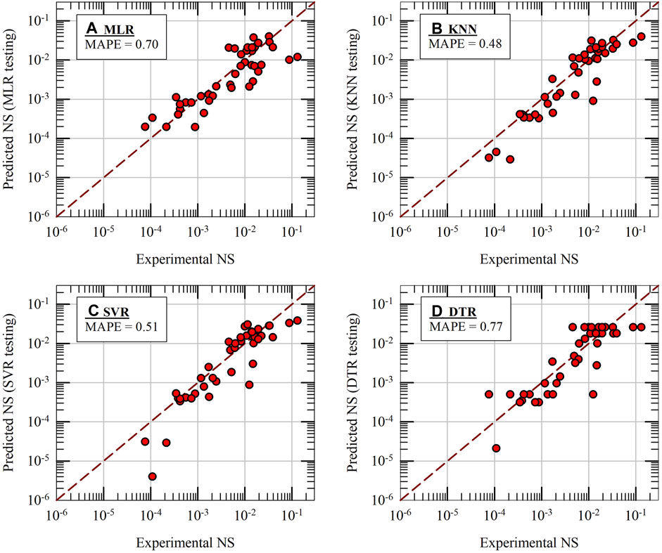
Figure 6. Machine learning model predictions of normalized settlement (NS) during initial testing of four base-ML models: (A) MLR, (B) KNN, (C) SVR and (D) DTR.

Figure 7

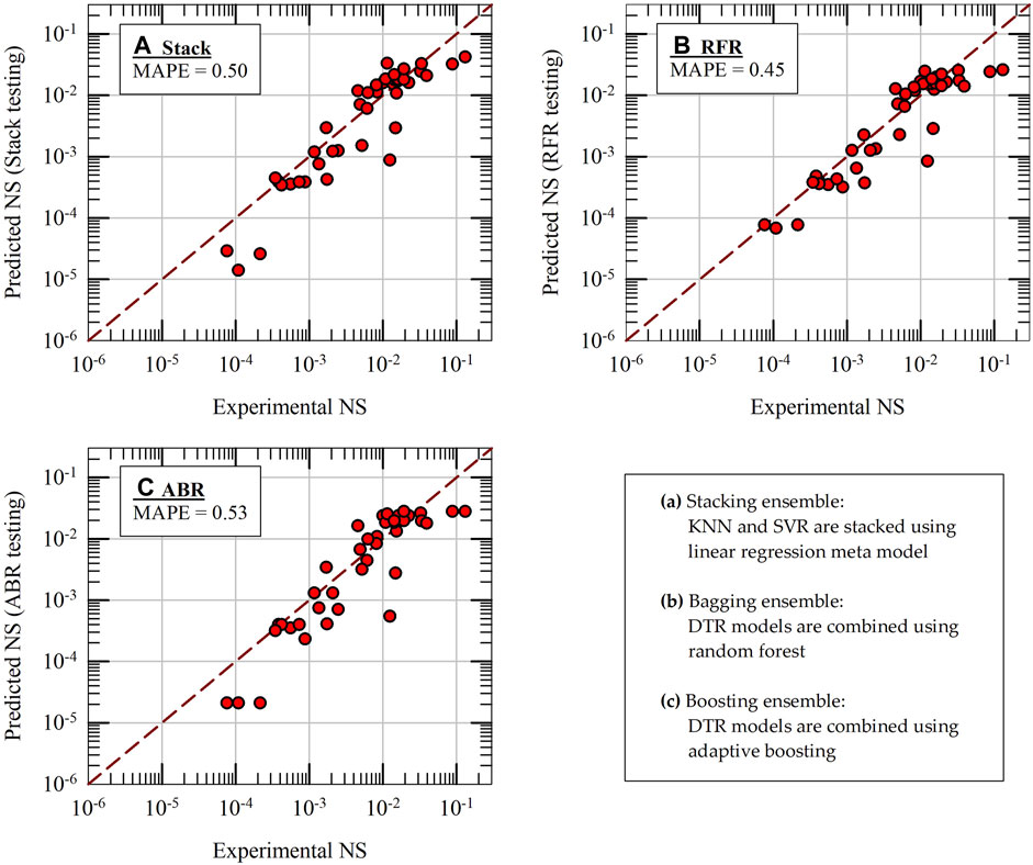
Figure 7. Machine learning model predictions of normalized settlement (NS) during initial testing of three ensemble-ML models: (A) Stack, (B) RFR and (C) ABR.

For the purpose of comparison, if a model always predicted the mean NS value (zero rule algorithm), it would yield an MAPE of 32.5 when tested on entire NS dataset. If a statistics-based simple linear regression model were run through the entire NS dataset, in log(NS)–log(I_a) space, it would yield an MAPE of 8.5 when tested on entire NS dataset. It should be noted that all the MAPE and MAE values are calculated based on the actual values of NS (not in log scale). These comparisons show that (i) there is significant scatter and randomness in NS data and (ii) when compared to the above-mentioned simple modes, the ML models presented in this paper perform better by an order of magnitude.

5.2 Sensitivity of machine learning models to input features

The RFR model’s “feature importances” function in Scikit-Learn quantifies the significance of each input feature based on how an input feature reduces uncertainty in data (as the nodes split the training dataset into smaller subsets while building the trees). The feature importance scores are normalized in such a way that the summation of feature importance scores of all input features is equal to 1.0. To investigate the effect of input features chosen in this study, twenty different RFR models are built by randomly selecting twenty different training datasets and the feature importance values are computed for each RFR model. The mean and standard deviation of the normalized feature importance scores are plotted in Figure 8 for each input feature. The rocking coefficient (C_r) has the greatest effect in reducing the uncertainty in data with a feature importance score of about 28%, and it is followed by slenderness ratio (h/B) and critical contact area ratio (A/A_c). This indicates that the geometry of the foundation and structure and bearing capacity of soil contribute more to the prediction of rocking-induced permanent settlement than the properties of earthquake ground motion. At the same time, the normalized feature importance scores of ground motion intensity parameters are around 10% each, indicating that they cannot be considered as redundant input features. The standard deviations of all the feature importance scores are less than 2% across 20 different random selection of training datasets, indicating the consistency of the RFR models built and the consistency of influence of each individual input feature on the prediction of NS.

Figure 8

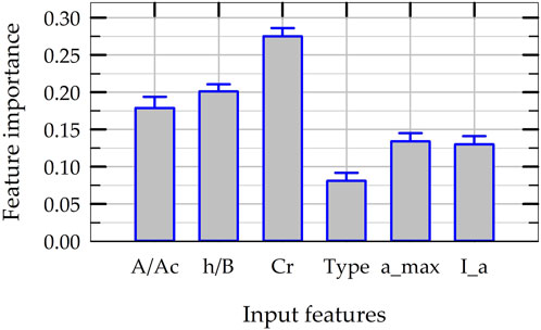
Figure 8. Significance of input features in terms normalized feature importance scores in the construction of RFR models.

5.3 Sensitivity of machine learning models to major hyperparameters

The k-fold cross validation technique is used to tune the hyperparameters of ML models. Instead of relying on just one value for MAPE, the k-fold cross validation technique uses multiple splits of data to obtain an average value for testing MAPE considering multiple different training datasets and testing datasets. It should be noted that only the initial training dataset is used for this k-fold cross validation tests to tune the hyperparameters (i.e., the multiple, reshuffled train-test split of data for this process considers only the training dataset as shown in the flowchart presented in Figure 5). In this study, 5-fold cross validation tests are carried out with three random reshuffling of data (i.e., 15 values for testing MAPE).

Figure 9 presents the variation of testing MAPE on y-axes and the values of hyperparameters on x-axes for different ML models, with every data point in the figures representing the average of 15 testing MAPE values. Based on the results presented in Figures 9A–C, the optimum value for k of KNN model, the optimum value for C of SVR model, and the optimum value for maximum depth of tree of DTR model are selected to be 3, 20 and 6, respectively. The aforementioned values are chosen for hyperparameters to minimize the testing MAPE values and to avoid overfitting and underfitting the training data. For example, any value smaller than the optimum value of k in KNN model, a value greater than the optimum value for C in SVR model, and a depth greater than the optimum value for maximum depth of DTR model would all overfit the training data. The opposite is true for underfitting the training data. For RFR and ABR models, the number of trees in the ensemble is varied while the maximum depth of the tree is fixed at 6. Based on the trend shown in Figure 9D, the optimum value for number of trees in both RFR and ABR ensemble is selected to be 100. It should be noted that, for the problem considered, the ML model predictions are not as sensitive to the other hyperparameters and they are set at their default values (the margin in SVR model = 0.1, maximum number of random features considered while building a tree in RFR model = 2, and the learning rate of ABR model = 0.1). Apart from hyperparameter tuning results, all other results of ML models presented in this paper are obtained using the optimum values of hyperparameters.

Figure 9

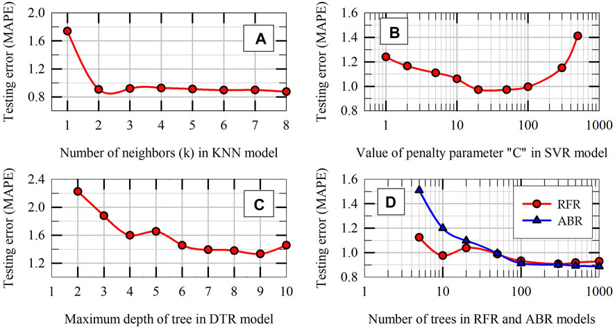
Figure 9. Hyperparameter tuning results: Average MAPE in k-fold cross validation tests on training dataset versus the hyperparameters of ML models: (A) KNN, (B) SVR, (C) DTR, and (D) RFR and ABR.

5.4 Initial evaluation of neural network models

ANN models with different architecture are developed, trained and tested. While the main structure of the ANN models is kept the same (multi-layer perceptron, fully-connected, sequential ANN models), the number of hidden layers and the number of neurons in each hidden layer are varied. The training and testing results of one of the ANN models are presented in Figures 10A, B, respectively. The same training dataset and testing dataset (same as the ones used for other ML models, described in section 5.1) are used to obtain the results presented in Figure 10. This particular ANN model has only one hidden layer with 20 neurons in the hidden layer (this is the optimum architecture obtained for the problem considered, as described in Section 5.5). During training, the ANN model starts with random values for network connection weights and it adjusts the weights using stochastic gradient descent algorithm until the error reaches a minimum. This particular results are obtained from one such random initialization of network connection weights. The final k-fold cross validation results presented in Section 5.7 removes the effects of this randomness by repeating the process multiple times and evaluating the average performance of the model. The testing MAPE of the ANN model is 0.46, which places the ANN model above all other ML models developed in this study in terms of prediction accuracy. It is interesting to note that the training MAPE of the ANN model is greater than the testing MAPE, which is not common in supervised machine learning.

Figure 10

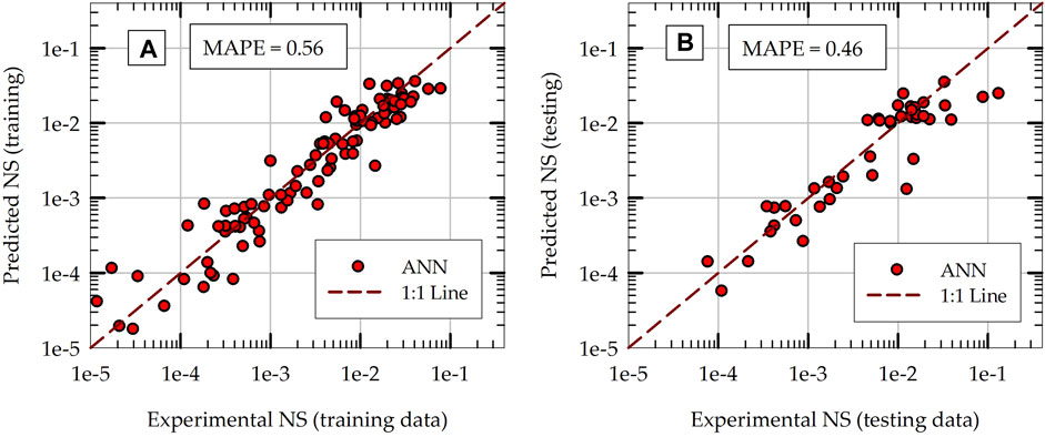
Figure 10. Comparisons of ANN model predictions with experimental values of normalized settlement (NS) during: (A) initial training phase and (B) initial testing phase.

5.5 Hyperparameter tuning of neural network models

The hyperparameters of the ANN model are tuned using 5-fold cross validation tests on training dataset. The number of hidden layers (L), the number of neurons in each hidden layer (N), the learning rate, and the number of epochs (iterations) are varied using grid search technique to optimize the values of these hyperparameters for the problem considered. The results obtained for average MAPE in 5-fold cross validation tests with the variation of hyperparameters are presented in Figure 11 for selected cases. As can be seen from Figure 11A, a shallow ANN model with only one hidden layer turns out to be the optimum for the problem considered. This is interesting, but not unusual. Research literature on neural networks suggest that a shallow network with only one hidden layer could, in theory, model even complicated, nonlinear data, provided that it has enough number of neurons in the hidden layer (Geron, 2019). Figure 11B shows that the accuracy of ANN model increases as the number of neurons in the hidden layer increases (average MAPE decreases); however the improvement in accuracy is not significant when the number of neurons increases beyond 20. In order to keep the model as simple as possible (least complexity) without scarifying the accuracy significantly, the optimum values for number of hidden layers and number of neurons in the hidden layer are selected to be 1 and 20, respectively. Similarly, based on the trends presented in Figures 11C, D, the optimum values for the learning rate of the SGD algorithm and number of echoes are selected as 0.01 and 200, respectively.

Figure 11

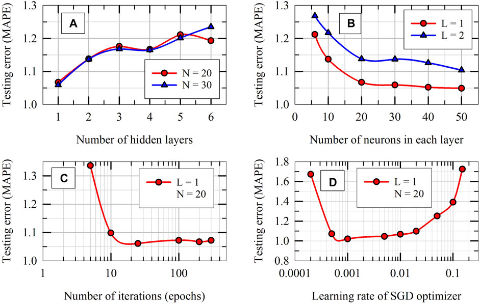
Figure 11. Hyperparameter tuning results of ANN model: Average MAPE in k-fold cross validation tests on training dataset versus hyperparameters of ANN model: (A) number of hidden layers, (B) number of neurons in each hidden layer, (C) number of epochs and (D) learning rate.

5.6 Effect of initial train-test split of data

Figure 12A presents a summary of training and testing MAPE of different ML models in the prediction of NS during initial evaluation of models. In Figure 12A, training error represents the performance of ML models when they are tested using the training dataset that is used to train the models (to quantify how much the models have learned from the training process). The consistency between the performances of different ML models are apparent: except for the baseline MLR model, all five nonlinear models included in Figure 12A have a testing MAPE that vary between 0.45 and 0.53. The training errors of these five models are smaller than the testing errors (this is expected especially when the data size is relatively small). Note that the training error for KNN model is not applicable, as KNN model stores the entire training dataset during training phase (the MAPE of distance-weighted KNN would be 0.0, if tested with the training data).

Figure 12

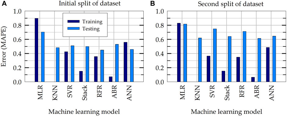
Figure 12. Mean absolute percentage error (MAPE) during training and testing of ML models: (A) initial random train-test split of dataset and (B) second random train-test split of dataset.

To investigate the effect of initial training and testing split of dataset, a second train-test split of data is created using a different value for the random state variable in the function used to split the data in scikit-learn. Figure 12B presents the training and testing errors of ML model when they are trained and tested on the second random split of train-test data. The training errors for both splits of data are relatively comparable, however the testing error on the second split of data of all ML models are noticeably greater than those on the first (initial) split of data. This indicates a bias in the initial split of data (especially testing dataset). To eliminate or reduce the bias resulting from a single train-test split of data, k-fold cross validation tests are carried out considering multiple random splits of the entire dataset. The results of this final k-fold cross validation tests are presented in next section.

5.7 Overall comparison of model performances

In order to compare the overall performance of all ML models developed in this study, final k-fold cross validation tests are carried out considering the entire dataset (5 folds with 3 repeats). For this purpose, the hyperparameters of all ML models are set at their optimum values and the models are trained and tested using multiple splits of dataset (please see the flowchart presented in Figure 5). Figure 13 presents the average testing MAPE of all ML models obtained during this k-fold cross validation tests along with the standard deviations of MAPE of each model as bar plots. As shown in Figure 13, the average MAPE of all nonlinear ML models are smaller than the baseline, linear MLR model for the prediction of NS. Except for the SVR model, the average MAPE of all the nonlinear ML models are smaller than 0.8. The average MAPE values of five nonlinear models (all but SVR) varies between 0.64 and 0.79, indicating the consistency in the performance of the ML models developed, though the models have different inductive biases (the assumptions based on which they learn or their learning objectives). The stacking ensemble model, which has the best average accuracy in final k-fold cross validation tests, improves the accuracy of prediction by about 33% when compared to the baseline MLR model (MAPE of 0.64 versus 0.96). Figure 14 presents the results of testing MAE in the predictions of NS in final k-fold cross validation tests in the same format as in Figure 13. Figure 14 indicates that the trend of MAE of different ML models follows a similar pattern as in Figure 13 for MAPE. The average MAE of all six nonlinear ML models vary between 0.005 and 0.006, once again indicating consistency among different ML models. This also implies that the ML models developed in this study have the potential to predict permanent settlement of rocking foundations with reasonable accuracy in practical applications.

Figure 13

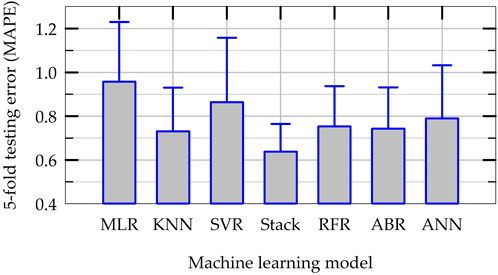
Figure 13. Summary results for the average and standard deviation of MAPE of ML models in final k-fold cross validation tests.

Figure 14

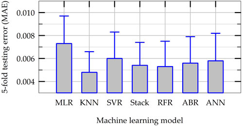
Figure 14. Summary results for the average and standard deviation of MAE of ML models in final k-fold cross validation tests.

Table 2 lists the values of average MAPE and MAE of all ML models during final k-fold cross validation tests. The MAPE of the statistics-based (non-ML) simple linear regression model for rocking-induced settlement is 8.5 (described in Section 5.1). The ML models developed in this study to predict the permanent settlement of rocking foundations improve that accuracy by 89%–92%. Also included in Table 2 are average values of a_20 index and a_50 index of model predictions in final k-fold cross validation tests. The a_20 index is defined as the ratio of number of predictions that fall within ±20% of the actual experimental values divided by the total number of predictions (Asteris et al., 2021). The a_50 index is defined in a similar way to quantify the ratio of predictions that fall within ±50% of the actual experimental values. The a_20 index of all ML models developed in this study, except the Stacking model, varies between 0.20 and 0.23. The relatively small values of a_20 index reflect the difficulty in predicting the rocking induced settlement accurately. It is interesting to note that the a_20 index of the Stacking model is the smallest (0.179) although its average MAPE is the best among all ML models in final k-fold cross validation tests. This suggests that Stacking model reduces the error in outliers of model predictions while the accuracy of model predictions that are closer to the actual values are not particularly high. Similarly, the a_50 index of the SVR model is the greatest (0.671) of all ML models while its average MAPE and MAE indicate that it is the least effective of all nonlinear models in terms of overall average accuracy. This suggests that most of the SVR model predictions are close to the actual values, while it produces relatively more outliers in predictions thus reducing the overall MAE and MAPE of predictions.

Table 2

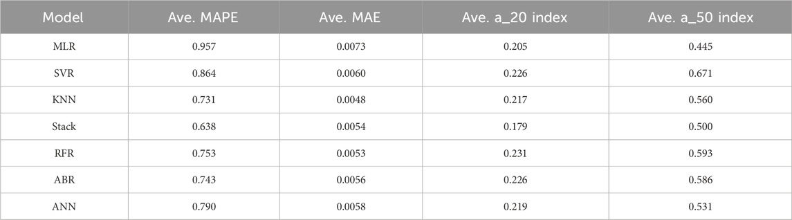
Table 2. Summary of average MAPE, MAE, a_20 index, and a_50 index of machine learning models in final k-fold cross validation tests of models.

6 Conclusion

The major achievement of this study is the development of multiple machine learning-based predictive models for settlement of shallow foundations due to rocking during earthquake loading. Though these ML models are trained and tested on a limited amount of available experimental data, they show promising predictive capabilities and they could possibly learn more and get even better in terms of their accuracy of predictions as more experimental data become available in the future. These ML models can be used with other analytical and numerical models and empirical relationships as complementary measures for estimating permanent settlement in practical applications of rocking foundations. The ML models presented here are (i) validated using experimental results, (ii) relatively easy to use (only six input features) and (iii) relatively fast and efficient compared to detailed finite element based modeling procedures. The major, specific conclusions drawn from this study include the following.

• Given the values of six input features (three rocking system capacity parameters, one binary feature for soil type and two earthquake ground motion parameters) that are relatively easily obtainable for foundation design in majority of seismic zones, the ML models presented herein can be used to estimate the permanent settlement of rocking foundations.

• The performances of all six nonlinear ML models developed in this study are relatively consistent in terms of prediction accuracy with their average MAPE varying between 0.64 and 0.86 in final k-fold cross validation tests.

• The overall average MAE in predictions of all nonlinear ML models are smaller than 0.006, implying that the ML models developed in this study have the potential to predict permanent settlement of rocking foundations with reasonable accuracy in practical applications.

• The ML models presented herein improve the accuracy of prediction by about 90% in comparison to a statistics based (non-ML) simple linear regression model (with MAPE = 8.5). In addition, the stacking ensemble model, which has the best average accuracy in final k-fold cross validation tests, improves the accuracy of prediction by about 33% when compared to the baseline MLR model (MAPE of 0.64 versus 0.96).

• Among the ANN model architectures considered, a shallow neural network (with only one hidden layer consisting of twenty neurons) is found to be the most suitable for the dataset analyzed without overfitting or underfitting the training data.

• Based on the feature importance values obtained from RFR ensemble model, it is found that the six input features chosen for ML models capture the permanent settlement of rocking foundations satisfactorily, and that the settlement of rocking foundations is more sensitive to soil-foundation system properties than to earthquake ground motion properties.

Data availability statement

The original contributions presented in the study are included in the article/Supplementary Material, further inquiries can be directed to the corresponding author.

Author contributions

SG: Conceptualization, Data curation, Formal Analysis, Funding acquisition, Investigation, Methodology, Project administration, Resources, Software, Supervision, Validation, Visualization, Writing–original draft, Writing–review and editing.

Funding

The author(s) declare that financial support was received for the research, authorship, and/or publication of this article. This research is funded by the US National Science Foundation (NSF) through award number CMMI-2138631.

Conflict of interest

The author declares that the research was conducted in the absence of any commercial or financial relationships that could be construed as a potential conflict of interest.

Publisher’s note

All claims expressed in this article are solely those of the authors and do not necessarily represent those of their affiliated organizations, or those of the publisher, the editors and the reviewers. Any product that may be evaluated in this article, or claim that may be made by its manufacturer, is not guaranteed or endorsed by the publisher.

Supplementary material

The Supplementary Material for this article can be found online at: https://www.frontiersin.org/articles/10.3389/fbuil.2024.1402619/full#supplementary-material

Abbreviations

ABR, Adaptive boosting regression model; a_max, Peak ground acceleration of earthquake; ANN, Artificial neural network regression model; A/A_c, Critical contact area ratio of rocking foundation; C_r, Rocking coefficient of rocking system; GBR, Gradient boosting regression model; h/B, Slenderness ratio of rocking system; I_a, Arias intensity of earthquake; KNN, k-nearest neighbors regression model; MAE, Mean absolute error; MAPE, Mean absolute percentage error; ML, Machine learning; MLR, Multivariate regression model; RFR, Random forest regression model; SVR, Support vector regression model.

References

Alkayem, N. F., Shen, L., Mayya, A., Asteris, P. G., Fu, R., Luzio, G. D., et al. (2024). Prediction of concrete and FRC properties at high temperature using machine and deep learning: a review of recent advances and future perspectives. J. Build. Eng. 83, 108369. doi:10.1016/j.jobe.2023.108369

CrossRef Full Text | Google Scholar

Allotey, N., and Naggar, M. H. (2003). Analytical moment-rotation curves for rigid foundations based on a Winkler model. Soil Dyn. Earthq. Eng. 23, 367–381. doi:10.1016/S0267-7261(03)00034-4

CrossRef Full Text | Google Scholar

Amjad, M., Ahmad, I., Ahmad, M., Wroblewski, P., Kaminski, P., and Amjad, U. (2022). Prediction of pile bearing capacity using XGBoost algorithm: modeling and performance evaluation. Appl. Sci. 9, 2126. doi:10.3390/app12042126

CrossRef Full Text | Google Scholar

Anastasopoulos, I., Gazetas, G., Loli, M., Apostolou, M., and Gerolymos, N. (2010). Soil failure can be used for seismic protection of structures. Bull. Earthq. Eng. 8, 309–326. doi:10.1007/s10518-009-9145-2

CrossRef Full Text | Google Scholar

Anastasopoulos, I., Loli, M., Georgarakos, T., and Drosos, V. (2013). Shaking table testing of rocking-isolated bridge pier on sand. J. Earthq. Eng. 17, 1–32. doi:10.1080/13632469.2012.705225

CrossRef Full Text | Google Scholar

Antonellis, G., Gavras, A. G., Panagiotou, M., Kutter, B. L., Guerrini, G., Sander, A., et al. (2015). Shake table test of large-scale bridge columns supported on rocking shallow foundations. J. Geotech. Geoenvironmental Eng. 141, 0001284. doi:10.1061/(ASCE)GT.1943-5606.0001284

CrossRef Full Text | Google Scholar

Arabpanahan, M., Mirghaderi, S. R., and Ghalandarzadeh, A. (2023). Experimental characterization of SDOF-embedded foundation systems with asymmetric interface condition. Acta Geotech. 2023, 02135–5. doi:10.1007/s11440-023-02135-5

CrossRef Full Text | Google Scholar

Armaghani, D. J., Asteris, P. G., Fatemi, S. A., Hasanipanah, M., Tarinejad, R., Rashid, A. S. A., et al. (2020). On the use of neuro-swarm system to forecast the pile settlement. Appl. Sci. 10, 1904. doi:10.3390/app10061904

CrossRef Full Text | Google Scholar

Asteris, P. G., Koopialipoor, M., Armaghani, D. J., Kotsonis, E. A., and Lourenco, P. B. (2021). Prediction of cement-based mortars compressive strength using machine learning techniques. Neural comput. Appl. 33, 13089–13121. doi:10.1007/s00521-021-06004-8

CrossRef Full Text | Google Scholar

Bapir, B., Abrahamczyk, L., Wichtmann, T., and Prada-Sarmiento, L. F. (2023). Soil-structure interaction: a state-of-the-art review of modeling techniques and studies on seismic response of building structures. Front. Built Environ. 9, 1120351. doi:10.3389/fbuil.2023.1120351

CrossRef Full Text | Google Scholar

Chatzigogos, C. T., Figini, R., Pecker, A., and Salencon, L. (2011). A macro element formulation for shallow foundations on cohesive and frictional soils. Int. J. Numer. Anal. methods Geomech. 35, 902–931. doi:10.1002/nag.934

CrossRef Full Text | Google Scholar

Deitel, P., and Deitel, H. (2020) Introduction to Python for computer science and data science. New York, NY, USA: Pearson Publishing.

Google Scholar

Deng, L., and Kutter, B. L. (2012). Characterization of rocking shallow foundations using centrifuge model tests. Earthq. Eng. Struct. Dyn. 41, 1043–1060. doi:10.1002/eqe.1181

CrossRef Full Text | Google Scholar

Deng, L., Kutter, B. L., and Kunnath, S. K. (2012). Centrifuge modeling of bridge systems designed for rocking foundations. J. Geotech. Geoenvironmental Eng. 138, 335–344. doi:10.1061/(ASCE)GT.1943-5606.0000605

CrossRef Full Text | Google Scholar

Diaz, E., Brotons, V., and Tomas, R. (2018). Use of artificial neural networks to predict 3-D elastic settlement of foundations on soils with inclined bedrock. Soils. Found. 58, 1414–1422. doi:10.1016/j.sandf.2018.08.001

CrossRef Full Text | Google Scholar

Drosos, V., Georgarakos, T., Loli, M., Anastsopoulos, I., Zarzouras, O., and Gazetas, G. (1012). Soil-foundation-structure interaction with mobilization of bearing capacity: experimental study on sand. J. Geotech. Geoenvironmental Eng. 138, 1369–1386. doi:10.1061/(ASCE)GT.1943-5606.0000705

CrossRef Full Text | Google Scholar

Ebid, A. M. (2021). 35 years of (AI) in geotechnical engineering: state of the art. Geotech. Geol. Eng. 39, 637–690. doi:10.1007/s10706-020-01536-7

CrossRef Full Text | Google Scholar

Figini, R., Paolucci, R., and Chatzigogos, C. T. (2012). A macro-element model for non-linear soil-shallow foundation-structure interaction under seismic loads: theoretical development and experimental validation on large scale tests. Earthq. Eng. Struct. Dyn. 41, 475–493. doi:10.1002/eqe.1140

CrossRef Full Text | Google Scholar

Gajan, S. (2021). Modeling of seismic energy dissipation of rocking foundations using nonparametric machine learning algorithms. Geotechnics 1, 534–557. doi:10.3390/geotechnics1020024

CrossRef Full Text | Google Scholar

Gajan, S. (2022). Data-driven modeling of peak rotation and tipping-over stability of rocking shallow foundations using machine learning algorithms. Geotechnics 2, 781–801. doi:10.3390/geotechnics2030038

CrossRef Full Text | Google Scholar

Gajan, S. (2023). Prediction of acceleration amplification ratio of rocking foundations using machine learning and deep learning models. Appl. Sci. 13, 12791. doi:10.3390/app132312791

CrossRef Full Text | Google Scholar

Gajan, S., and Godagama, B. (2019). Seismic performance of bridge-deck-pier-type-structures with yielding columns supported by rocking foundations. J. Earthq. Eng. 26, 640–673. doi:10.1080/13632469.2019.1692737

CrossRef Full Text | Google Scholar

Gajan, S., and Kutter, B. L. (2008). Capacity, settlement, and energy dissipation of shallow footings subjected to rocking. J. Geotech. Geoenvironmental Eng. 134, 1129–1141. doi:10.1061/(ASCE)1090-0241(2008)134:8(1129)

CrossRef Full Text | Google Scholar

Gajan, S., and Kutter, B. L. (2009). Contact interface model for shallow foundations subjected to combined cyclic loading. J. Geotech. Geoenvironmental Eng. 135, 407–419. doi:10.1061/(ASCE)1090-0241(2009)135:3(407)

CrossRef Full Text | Google Scholar

Gajan, S., Phalen, J. D., Kutter, B. L., Hutchinson, T. C., and Martin, G. (2005). Centrifuge modeling of load-deformation behavior of rocking shallow foundations. Soil Dyn. Earthq. Eng. 25, 773–783. doi:10.1016/j.soildyn.2004.11.019

CrossRef Full Text | Google Scholar

Gajan, S., Raychowdhury, P., Hutchinson, T. C., Kutter, B. L., and Stewart, J. P. (2010). Application and validation of practical tools for nonlinear soil-foundation interaction analysis. Earthq. Spectra 26, 111–129. doi:10.1193/1.3263242

CrossRef Full Text | Google Scholar

Gajan, S., and Saravanathiiban, D. S. (2011). Modeling of energy dissipation in structural devices and foundation soil during seismic loading. Soil Dyn. Earthq. Eng. 31, 1106–1122. doi:10.1016/j.soildyn.2011.02.006

CrossRef Full Text | Google Scholar

Gajan, S., Soundararajan, S., Yang, M., and Akchurin, D. (2021). Effects of rocking coefficient and critical contact area ratio on the performance of rocking foundations from centrifuge and shake table experimental results. Soil Dyn. Earthq. Eng. 141, 106502. doi:10.1016/j.soildyn.2020.106502

CrossRef Full Text | Google Scholar

Gavras, A. G., Kutter, B. L., Hakhamaneshi, M., Gajan, S., Tsatsis, A., Sharma, K., et al. (2020). Database of rocking shallow foundation performance: dynamic shaking. Earthq. Spectra 36, 960–982. doi:10.1177/8755293019891727

CrossRef Full Text | Google Scholar

Gavras, A. G., Kutter, B. L., Hakhamaneshi, M., Gajan, S., Tsatsis, A., Sharma, K., et al. (2023). FoRDy: rocking shallow foundation performance in dynamic experiments. DesignSafe-CI 2023. doi:10.13019/3rqyd929

CrossRef Full Text | Google Scholar

Geron, A. (2019) Hands-on machine learning with Scikit-Learn, Keras, and TensorFlow: concepts, tools and techniques to build intelligent systems. Sebastopol, CA, USA: O’Reilly Media Inc.,

Google Scholar

Goh, A. T. C., and Goh, S. H. (2007). Support vector machines: their use in geotechnical engineering as illustrated using seismic liquefaction data. Comput. Geotech. 34, 410–421. doi:10.1016/j.compgeo.2007.06.001

CrossRef Full Text | Google Scholar

Hakhamaneshi, M., Kutter, B. L., Deng, L., Hutchinson, T. C., and Liu, W. (2012). “New findings from centrifuge modeling of rocking shallow foundations in clayey ground,” in Proc. Geo-Congress 2012, Oakland, CA, USA.

CrossRef Full Text | Google Scholar

Hakhamaneshi, M., Kutter, B. L., Gavras, A. G., Gajan, S., Tsatsis, A., Liu, W., et al. (2020). Database of rocking shallow foundation performance: slow-cyclic and monotonic loading. Earthq. Spectra 36, 1585–1606. doi:10.1177/8755293020906564

CrossRef Full Text | Google Scholar

Hamidpour, S., Shakib, H., Paolucci, R., Correia, A. A., and Soltani, M. (2022). Empirical models for the nonlinear rocking response of shallow foundations. Bull. Earthq. Eng. 20, 8099–8122. doi:10.1007/s10518-022-01449-1

CrossRef Full Text | Google Scholar

Irani, A. E., Bonab, M. H., Sarand, F. B., and Katebi, H. (2023). Overall improvement of seismic resilience by rocking foundation and trade-off implications. Int. J. Geosynth. Ground Eng. 9, 40. doi:10.1007/s40891-023-00454-x

CrossRef Full Text | Google Scholar

Jeremiah, J. J., Abbey, S. J., Booth, C. A., and Kashyap, A. (2021). Results of application of artificial neural networks in predicting geo-mechanical properties of stabilized clays – a review. Geotechnics 1, 144–171. doi:10.3390/geotechnics1010008

CrossRef Full Text | Google Scholar

Karpatne, A., Atluri, G., Faghmous, J. H., Steinbach, M., Banerjee, A., Ganguly, A., et al. (2017). Theory-guided data science: a new paradigm for scientific discovery from data. IEEE Trans. Knowl. Data Eng. 29, 2318–2331. doi:10.1109/TKDE.2017.2720168

CrossRef Full Text | Google Scholar

Ko, K.-W., Ha, J.-G., Park, H.-J., and Kim, D.-S. (2019). Centrifuge modeling of improved design for rocking foundation using short piles. J. Geotech. Geoenvironmental Eng. 145, 5606–0002064. doi:10.1061/(ASCE)GT.1943-5606.0002064

CrossRef Full Text | Google Scholar

Kramer, S. (1996) Geotechnical earthquake engineering. Upper Saddle River, NJ, USA: Prentice Hall Inc.

Google Scholar

Loli, M., Knappett, J. A., Brown, M. J., Anastasopoulos, I., and Gazetas, G. (2014). Centrifuge modeling of rocking-isolated inelastic RC bridge piers. Earthq. Eng. Struct. Dyn. 43, 2341–2359. doi:10.1002/eqe.2451

PubMed Abstract | CrossRef Full Text | Google Scholar

Mozumder, R. A., and Laskar, A. I. (2015). Prediction of unconfined compressive strength of geopolymer stabilized clayey soil using Artificial Neural Network. Comput. Geotech. 69, 291–300. doi:10.1016/j.compgeo.2015.05.021

CrossRef Full Text | Google Scholar

Paolucci, R., Shirato, M., and Yilmaz, M. T. (2008). Seismic behaviour of shallow foundations: shaking table experiments vs numerical modelling. Earthq. Eng. Struct. Dyn. 37, 577–595. doi:10.1002/eqe.773

CrossRef Full Text | Google Scholar

Pelekis, I., McKenna, F., Madabhushi, G. S. P., and DeJong, M. J. (2021). Finite element modeling of buildings with structural and foundation rocking on dry sand. Earthq. Eng. Struct. Dyn. 50, 3093–3115. doi:10.1002/eqe.3501

CrossRef Full Text | Google Scholar

Pham, B. T., Bui, D. T., and Prakash, I. (2017). Landslide susceptibility assessment using bagging ensemble based alternating decision trees, logistic regression and J48 decision trees methods: a comparative study. Geotech. Geol. Eng. 35, 2597–2611. doi:10.1007/s10706-017-0264-2

CrossRef Full Text | Google Scholar

Sharma, K., and Deng, L. (2019). Characterization of rocking shallow foundations on cohesive soil using field snap-back tests. J. Geotech. Geoenvironmental Eng. 145, 0002114. doi:10.1061/(ASCE)GT.1943-5606.0002114

CrossRef Full Text | Google Scholar

Sharma, K., and Deng, L. (2020). Field testing of rocking foundations in cohesive soil: cyclic performance and footing mechanical response. Can. Geotech. J. 57, 828–839. doi:10.1139/cgj-2018-0734

CrossRef Full Text | Google Scholar

Soong, T. T., and Spencer, Jr. B. F. (2002). Supplemental energy dissipation: state-of-the-art and state-of-the-practice. Eng. Struct. 24, 243–259. doi:10.1016/S0141-0296(01)00092-X

CrossRef Full Text | Google Scholar

Symans, M. D., Charney, F. A., Whittaker, A. S., Constantinou, M. C., Kircher, C. A., Johnson, M. W., et al. (2008). Energy dissipation systems for seismic applications: current practice and recent developments. J. Struct. Eng. 134, 3–21. doi:10.1061/(ASCE)0733-9445(2008)134:1(3)

CrossRef Full Text | Google Scholar

Tsatsis, A., and Anastasopoulos, I. (2015). Performance of rocking systems on shallow improved sand: shaking table testing. Front. Built Environ. 1, 00009. doi:10.3389/fbuil.2015.00009

CrossRef Full Text | Google Scholar

Xiong, J., Pei, T., and Qiu, T. (2023). “A machine learning-based method with integrated physics knowledge for predicting bearing capacity of pile foundations,” in Proc. Geo-Congress 2023, Los Angeles, CA, USA.

CrossRef Full Text | Google Scholar