 María Quiroz
 Cristóbal Gálmez
 Gastón A. Fermandois
- 1Departamento de Obras Civiles, Universidad Técnica Federico Santa María, Valparaíso, Chile
- 2Department of Engineering, City, University of London, London, United Kingdom
Real-time hybrid simulation (RTHS) is a powerful and highly reliable technique integrating experimental testing with numerical modeling for studying rate-dependent components under realistic conditions. One of its key advantages is its cost-effectiveness compared to large-scale shake table testing, which is attained by selectively conducting experimental testing on critical parts of the analyzed structure, thus avoiding the assembly of the entire system. One of the fundamental advancements in RTHS methods is the development of multi-dimensional dynamic testing. In particular, multi-axial RTHS (maRTHS) aims to prescribe multi-degree-of-freedom (MDOF) loading from the numerical substructure over the test specimen. Under these conditions, synchronization is a significant challenge in multiple actuator loading assemblies. This study proposes a robust and decentralized adaptive compensation (RoDeAC) method for the next-generation maRTHS benchmark problem. An initial calibration of the dynamic compensator is carried out through offline numerical simulations. Subsequently, the compensator parameters are updated in real-time during the test using a recursive least squares adaptive algorithm. The results demonstrate outstanding performance in experiment synchronization, even in uncertain conditions, due to the variability of reference structures, seismic loading, and multi-actuator properties. Notably, this achievement is accomplished without needing detailed information about the test specimen, streamlining the procedure and reducing the risk of specimen deterioration. Additionally, the tracking performance of the tests closely aligns with the reference structure, further affirming the excellence of the outcomes.
1 Introduction
Real-time hybrid simulation (RTHS) is a powerful and highly reliable technique that integrates experimental testing with numerical modeling (Nakashima et al., 1992). As a real-time variant of pseudo-dynamic testing, RTHS enables studying rate-dependent components under realistic conditions. One of its key advantages is its cost-effectiveness, which is achieved by selectively conducting experimental testing on critical parts of the analyzed structure, thus avoiding the assembly of the entire system. The laboratory essays primarily focus on the experimental substructure, while the well-known portions are accurately represented through numerical modeling within a computer interface. This innovative approach offers a practical and efficient means of evaluating structural behavior and performance, making RTHS a valuable tool for various engineering applications (Asai et al., 2013; Botelho and Christenson, 2014; Ghaffary and Mohammadi, 2019).
In RTHS, actuators are typically utilized to impose the numerical response over the experimental parts. Simultaneously, the experimental forces are measured and fed back into the numerical substructure. However, the procedure must enforce real-time compatibility and equilibrium at the hybrid interface (Dermitzakis and Mahin, 1985). Therefore, seamless synchronization between the numerical and experimental components demands meticulous time management to avoid inaccurate and unstable responses (Horiuchi et al., 1996). Several challenges arise in this process, including the time required for calculations, the precise application of displacements using actuators, and the digital acquisition of measured forces within extremely small time increments. As a consequence, researchers have developed control techniques to compensate for the actuator’s dynamics and minimize tracking errors to address the synchronization challenge. Early methods are based on polynomial extrapolation, assuming a constant delay (Horiuchi et al., 1999). Other methods are based on the inverse of the first-order transfer function, which represents the transfer system (Chen and Ricles, 2010). Models with higher-order transfer functions are used for model-based techniques (Carrion and Spencer, 2007). Model-based feedforward and feedback compensation (Phillips and Spencer Jr, 2012) have excellent results if a good plant model is available to design the controller. However, there are no guarantees of accuracy or stability when significant uncertainty exists in the model.
An alternative to traditional dynamic compensators is the adaptive compensation algorithm, which has been proposed to address the uncertainty or significant non-linearity in the control plant. Some of them use a first-order transfer function with adapting parameters to represent the transfer system, where the adaptation depends on a frequency-domain evaluation index (FEI) analysis of commanded and measured signals, such as adaptive phase-lead compensation (Tao and Mercan, 2019) or windowed FEI compensation (Xu et al., 2019). Other methods, like adaptive time series (Chae et al., 2013) and conditional adaptive time series (Palacio-Betancur and Gutierrez Soto, 2019), estimate the plant through Taylor series expansion and adjust the parameters in the time domain. Adaptive model-based compensation (Chen et al., 2015) consists of an estimate of the plant in the frequency domain; then, compensation is implemented in the time domain using numeric derivatives of the commanded signal and adaptation based on the gradient. Wang et al. (2020) used adaptive delay compensation based on a discrete system model where the compensation commands are generated using the target, measured, and previous displacements. Ning et al. (2020) used an adaptive model-based control strategy with feedforward and feedback control and added a Kalman filter for parameter estimation.
The necessity of carrying out realistic experiments has been the principal factor that led to the development of multi-dimensional testing in RTHS, giving way to multi-axial RTHS (maRTHS). These tests prescribe multiple-degree-of-freedom (MDOF) responses from the numerical substructure into the test specimen, which requires multiple hydraulic actuators to prescribe all the motions over the experimental substructure (Fermandois and Spencer, 2017). As the complexity of the problem increases, enforcing a higher number of degrees of freedom (DOFs) at a given interface boundary condition may require incorporating supplementary physical components or multi-axial loading systems, such as high-stiff links or couplers. The assemblage of multi-axial hydraulic actuators demands nonlinear coordinate transformations, adding complexity due to nonlinearities, uncertainties, and internal coupling, among other complexities. Consequently, conducting experiments with such multi-axial setups and achieving precise synchronization remain a considerable challenge, making developing and validating effective multiple-input multiple-output (MIMO) control strategies urgently necessary (Najafi et al., 2023). Moreover, most of the previously mentioned compensation algorithms have been tested only on single-actuator problems (Silva et al., 2020).
Meanwhile, the compensation algorithms in RTHS predominantly use displacement control. Two primary real-time control approaches are employed for multi-actuator devices: centralized and decentralized (Najafi et al., 2023). The former adopts a more comprehensive approach concerning the interaction between actuators, treating multiple actuator loading platforms as MIMO systems in Cartesian coordinates and addressing system-wide actuator dynamics (Fermandois and Spencer, 2017). However, the design and implementation of centralized controllers can pose challenges due to the many parameters requiring fine-tuning. On the contrary, decentralized control is preferred due to its comparatively simple design, enabling dynamic compensators initially crafted for single-input, single-output systems in actuator coordinates (Najafi et al., 2020). However, it should be noted that such controllers may exhibit limitations when grappling with experiments characterized by significant multi-actuator and specimen dynamic coupling.
Hence, this study proposes a robust and decentralized adaptive compensation (RoDeAC) method for maRTHS experimental tests and is developed and validated through the next-generation maRTHS benchmark problem (Condori et al., 2023). The proposed method can be designed independently from the experimental substructure, avoiding unnecessary initial identification testing that may cause premature damage to the physical specimens before the maRTHS test. By incorporating adaptation over the compensation layer, this technique maintains excellent synchronization even in the presence of uncertain and time-varying properties of the specimen. We propose defining the initial conditions and parameters of the controller using only knowledge of the transfer system through a model of the multi-actuator loading assembly, including the interaction with the test specimen. The initial calibration of the controller is carried out through offline simulations, where the decentralized multi-actuator is trained with assumed perturbed structural loading and coupling values.
This study is structured as follows: Section 2 presents the problem formulation corresponding to the virtual maRTHS benchmark problem. Section 3 describes the methodology employed to compensate the actuators involved in maRTHS using a recursive least squares (RLS) adaptive compensator. Section 4 details the initial calibration of RoDeAC for the benchmark problem. Section 5 provides the results of the numerical simulations and their comparisons regarding the benchmark. Finally, Section 6 discusses the principal findings and final remarks of this study.
2 Problem description
2.1 Reference structure
The maRTHS benchmark problem (Condori et al., 2023) is considered in this study for the development and validation of a proposed robust compensation algorithm that is capable of rejecting uncertainties mainly due to specimen-multiactuator interactions. In this benchmark problem, a three-story, three-bay, planar steel moment frame is chosen as the reference structure, as shown in Figure 1. Steel shapes and tributary gravity loads are provided to compute masses for dynamic transient analyses.
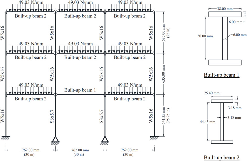
Figure 1. Reference structure considered for the maRTHS benchmark problem (Condori et al., 2023).
A multi-degree-of-freedom (MDOF) linear-time-invariant (LTI) numerical model is provided for the reference structure. The structural system has linear-elastic behavior and three degrees of freedom (DOFs) per node: two translational DOFs along the global
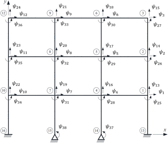
Figure 2. Numeration of DOF of the reference structure (adapted from Condori et al., 2023).
The equation of motion (EOM) is given by Eq. 1:
where
As a consequence, the first five natural frequencies are
2.2 Substructuring
In the context of RTHS, instead of solving the EOM for the entire reference domain, a process known as substructuring can be employed to subdivide the domain into smaller subdomains, such that the order of large and complex structural systems is reduced for efficient computations (Dermitzakis and Mahin, 1985). Each subdomain can be solved independently, provided that coupling between components is enforced through compatibility and equilibrium conditions at their interfaces.
In the benchmark case, the domain is decomposed into two non-overlapping subdomains, i.e.,
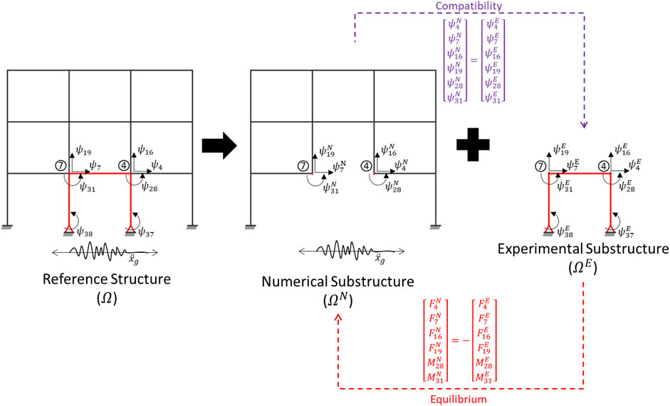
Figure 3. Partition considered for the maRTHS benchmark problem. (adapted from Condori et al., 2023).
If we assume the frame exhibits linear elastic behavior, the matrices for partitioned mass, damping, and stiffness can be expressed as the combination of numerical components (denoted with the superscript “
The terms associated with the experimental substructure can be arranged into the right-hand side of the EOM as described in Eqs 4, 5:
Here,
Due to boundary conditions, both compatibility and equilibrium must be satisfied, as mentioned previously in this section. The first condition assures that the displacements at the interface of the subdomains are the same, allowing maRTHS to impose the numerical displacements (and their time derivatives) into the experimental substructure. In this case, they are given by the following DOFs:
In maRTHS, the previously mentioned process is repeated until the simulation reaches the final simulation time
In this benchmark problem, the EOM is integrated using the fourth-order Runge–Kutta integration scheme incorporated in Simulink (ode4), and the sampling frequency
2.3 Transfer system
In this section, we explain the transfer system, which consists of a set of servo-hydraulic actuators. First, the vertical DOFs along the global coordinate
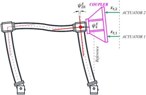
Figure 4. Description of the experimental setup employed for the maRTHS benchmark problem (adapted from Condori et al., 2023).
The servo-hydraulic actuators are Shore Western 910D series, with a nominal force capacity of 9.34 kN and a stroke of ±63 mm, with a built-in linear variable differential transformer (LVDT) transducer that collects measurements of linear displacements, and two load cells (Interface, 1000 series) with a nominal force capacity of 11.2 kN, providing instantaneous force measurements. These hydraulic actuators operate with a hydraulic power supply (MTS pump) with a capacity of up to 680 L/min at 206 Bar. Meanwhile, the coupler, made from SAE 1018 low-carbon steel plates, has a mass of 17.9 kg. Furthermore, it is worth mentioning that the benchmark problem statement does not explicitly report the moment of inertia with respect to the center of mass of the coupler since it is assumed that these inertial effects were indeed incorporated when they conducted system identification of the control plant (i.e., transfer system connected to the test specimen).
2.3.1 Coupler coordinate transformation
The actuators enforce translations into the physical specimen. Therefore, a coordinate transformation is required between the translational and rotational DOFs of the numerical substructure in Cartesian coordinates and the displacements on actuator coordinates. The following four important assumptions are made:
i. The coupler deformations are negligible (i.e., rigid body motion).
ii. The vertical motion of the nodes is neglected.
iii. The rotations of the column-beam joints are small because the behavior of the frame is limited to linear elasticity.
iv. The connection of the coupler to the column-beam joint provided by the high-strength bolts is rigid; hence, the deformations are negligible.
Figure 5 shows the kinematics of the rigid coupler, illustrated by the blue dashed triangle in the default position and with a green continuous triangle for finite rotations. Considering the geometry shown in Figure 5, the coordinate transformation can be calculated from Eq. 6:
where
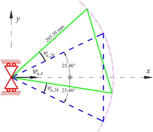
Figure 5. Rigid coupler kinematics (adapted from Condori et al., 2023).
Meanwhile,
2.3.2 Control plant dynamics
The control plant (i.e., transfer system + specimen) has two inputs
where
where
The nominal values for the transfer function parameters of Eq. 10 are identified using experimental data using four spectral densities of band-limited white noise (BLWN) signals as inputs to the control plant. The first two tests were implemented using a 0–100 Hz BLWN signal to only one of the actuators while setting zero for the other one, thus allowing the calculation of the columns of the experimental transfer matrix. Then, a two-pole transfer function model is fitted to the experimental frequency response functions (FRFs) (Condori et al., 2023). Then, transfer function parameters are modeled as random variables with a normal distribution to consider uncertainty in the system (e.g., geometry, material properties, eccentricity, and nonlinearities). Random variations in the poles and zeros of the nominal plant model generate these differences by introducing changes from a standard normal distribution sampling process, which creates a family of FRFs where any FRF member represents a potential control plant. Finally, the nominal values and standard deviation of each parameter are presented in Table 1 and drawn in Figure 6.
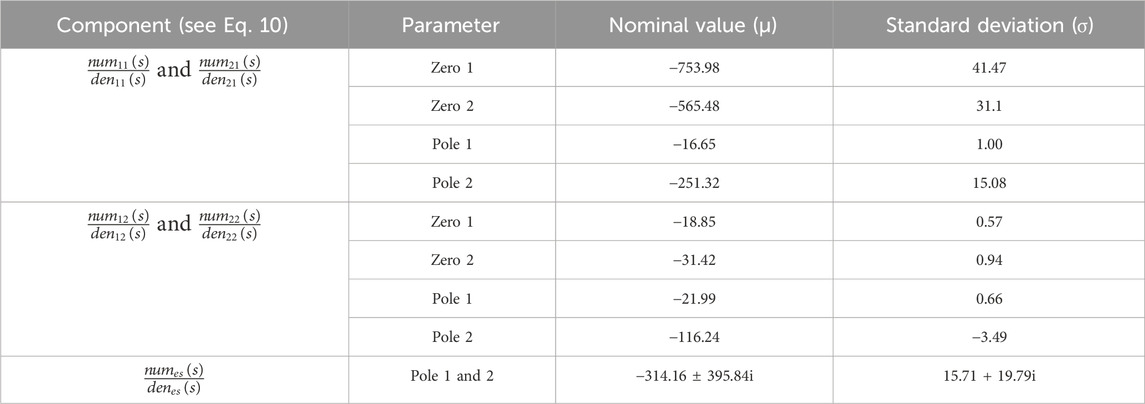
Table 1. Parameter uncertainty definition (Condori et al., 2023).
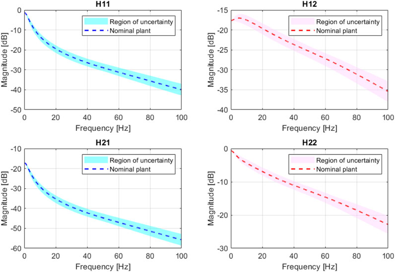
Figure 6. FRF regions for the plant model uncertainty. (adapted from Condori et al., 2023).
3 Methodology
3.1 Recursive least squares adaptive compensation
In this study, the recursive least squares adaptive compensation (RLS-AC) initially proposed by Galmez and Fermandois (2022) for maRTHS systems is considered for application in the context of the maRTHS benchmark problem to provide a detailed comparison in terms of its performance and robustness with the benchmark results. The compensation is employed in a decentralized manner for reference tracking of multiple actuators in maRTHS. In this way, each actuator is treated as an independent control plant, and the goal of each compensator is to minimize the tracking error between a target signal
The RLS-AC technique consists of the design of two fundamental components: (i) a feedforward compensator, responsible for reference-tracking performance; and (ii) a recursive parameter estimator, which aims to provide sufficient robustness to the closed-loop system under unwanted disturbances and measurement noises. Both the feedforward and parameter estimators are designed independently, based on the nominal control plant model defined in Section 2.3. A schematic representation of the RLS-AC architecture employed in RTHS is presented in Figure 7.
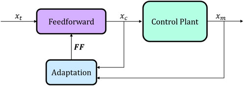
Figure 7. Main architecture of RLS adaptive compensation.
In this study, three discrete-time signals are considered in the RLS-AC architecture: (i) target signal
Here, the command signal to the actuator can be obtained from the Eq. 11:
where
where
where
The initial adaptive parameter
where
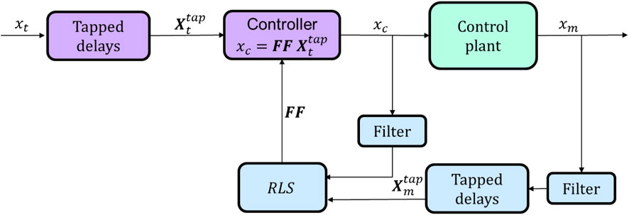
Figure 8. Flowchart of the RLS adaptive compensator.
3.2 Decentralized adaptive compensator for maRTHS testing
The algorithm mentioned before is applied to each actuator in a decentralized manner; this means that for each actuator, there is a different compensator that works independently from each other, with unique initial parameters and adaptation processes, as shown in the Simulink diagram in Figure 9A. The independence of this compensation algorithm in maRTHS, even assuming identical actuators, is proved by Galmez and Fermandois (2022) as the parameter adaptation process is different for each one of the actuators. Figure 9B shows a block diagram of the implemented RoDeAC for virtual maRTHS.
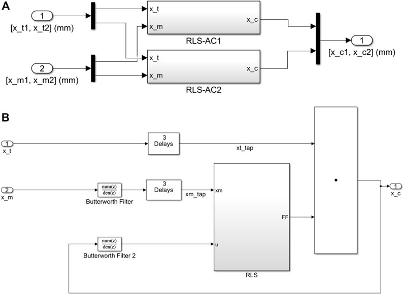
Figure 9. Block diagram of the RoDeAC in actuator coordinates: (A) maRTHS implementation and (B) subsystem considered for each actuator.
4 Calibration of robust decentralized adaptive compensators
4.1 Initial parameters
Offline tests are required to provide the necessary data for initializing the RLS-AC method and assessing the method’s performance for prescribed desired displacement loading. Then, a Simulink implementation is used, as shown in Figure 10, where the structural response is measured in an open-loop system without the feedback of the experimental forces back to the numerical substructure. In this case, we use the multi-actuator models described in Section 2.3.2, which provides information about the control system with the numerical substructure subjected to seismic excitation. Notably, this process can be carried out even without any interaction with the test specimen. Then, the structural response is imposed on the specimen (
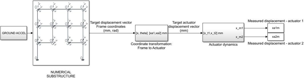
Figure 10. Block diagram of the offline calibration testing.
Different scenarios are used to analyze the initial parameters’ dispersion for the offline calibration. Therefore, three different earthquakes (El Centro, 1940; Kobe, 1995; and Morgan, 1984) with different seismic intensity measures (20%, 40%, and 60% PGA scales) are used to calculate different
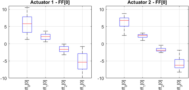
Figure 11. Statistical dispersion of the initial values for parameter
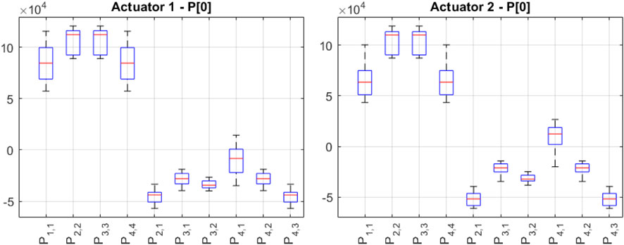
Figure 12. Statistical dispersion of the initial values for parameter
Note that, under the assumption of different conditions, the values for the initial parameter values change. Moreover, in this case, different values for parameters
Finally, the mean values are considered in this study for the initialization of each parameter and are presented in Eqs 19–22.
• Actuator 1:
• Actuator 2:
4.2 Forgetting factor
The forgetting factor is used to weaken the influence of older data on the estimated parameter values. This means that as simulation time increases, the old data are discarded exponentially by the parameter estimator of the adaptive compensator (Ioannou and Sun, 2012). A small forgetting factor decreases the impact of older data on the identified parameters and is thus more suitable for time-varying systems. However, small forgetting factors may cause serious fluctuations in the identified parameters (Wang et al., 2020). To observe how this parameter affects our virtual maRTHS, graphs illustrating the
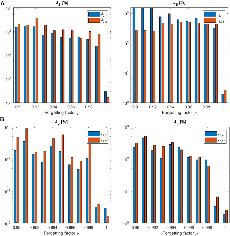
Figure 13. Influence of the forgetting factor on the performance of virtual maRTHS, ranging from (A) 0.9 to 1; and (B) 0.99 to 1.
5 Results
The tracking controller was implemented in Simulink using a reference model block provided by the benchmark problem (Condori et al., 2023). Simulations were conducted in real-time using MATLAB and Simulink R2021a with Simulink Desktop Real-Time version 5.12.0, running on a 64-bit computer with an Intel i7-9750H CPU, 16 GB of RAM, and the Windows 10 version 22H2 operating system. The nominal and 100 perturbed control plants were studied to assess the performance and robustness of the controller employed.
5.1 Compensation of multi-actuator dynamics
To study the tracking performance of the RoDeAC in the time domain, the seismic excitation chosen was the 1940 EL Centro earthquake, with 40% scaled PGA intensity. Figure 14 shows the target (
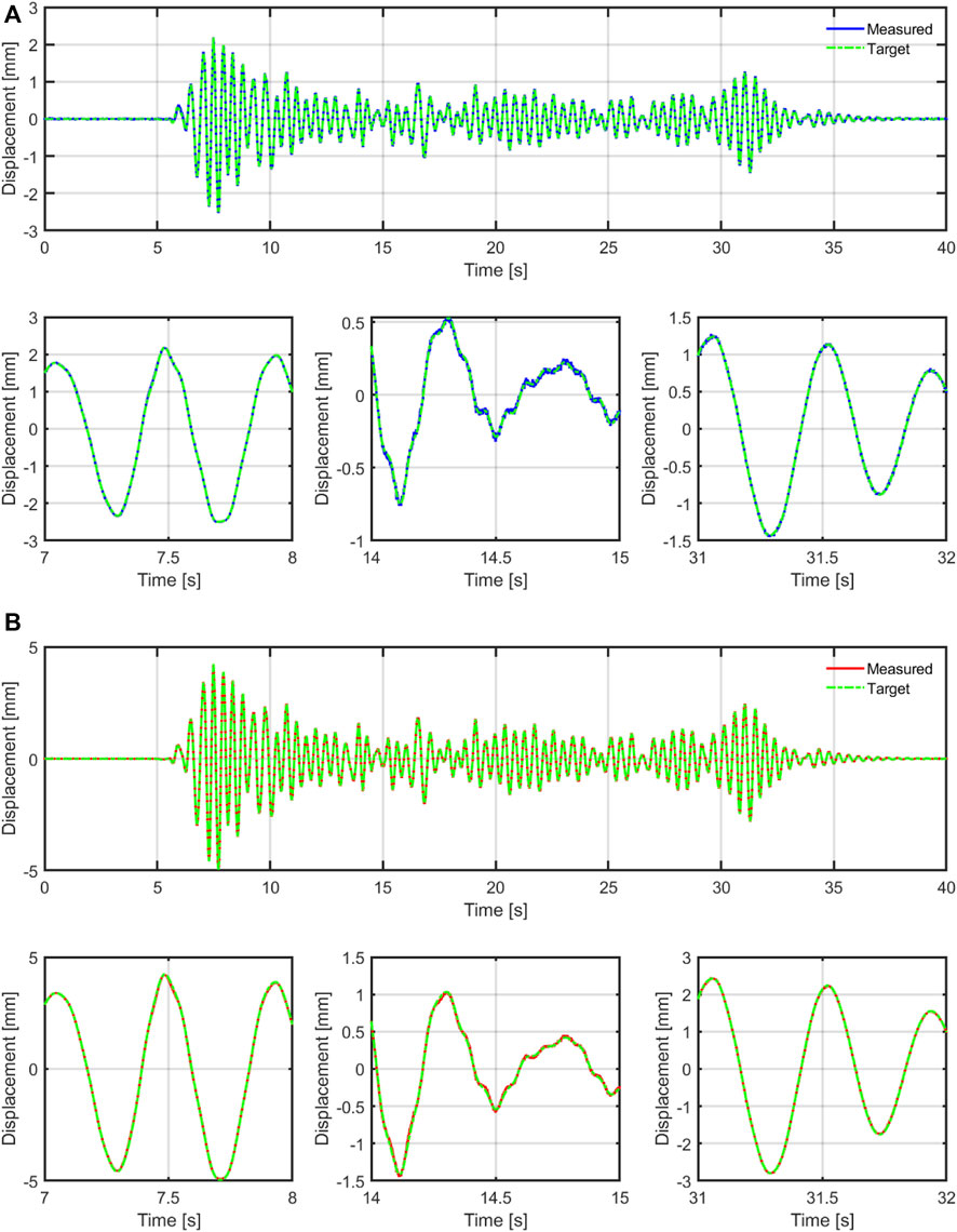
Figure 14. maRTHS tracking performance in actuator coordinates. Target and measured actuator displacement for (A) actuator 1 and (B) actuator 2.
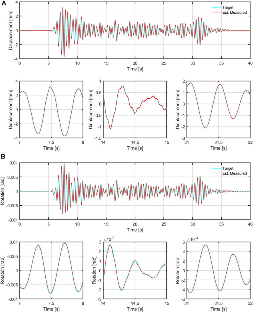
Figure 15. maRTHS tracking performance at the interface node (frame coordinates). Target numerical substructure vs. estimated experimental responses for (A) translational DOF (
Furthermore, Figure 16 presents the evolution of parameter
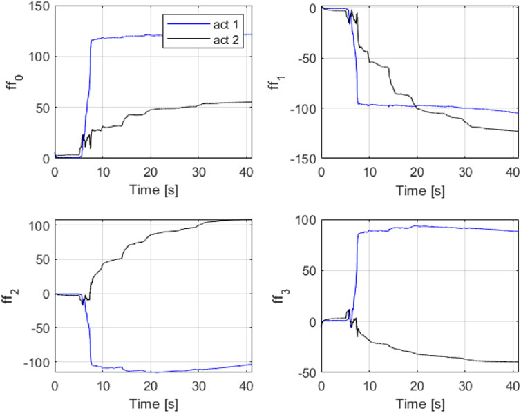
Figure 16. Evolution of RoDeAC adaptive parameters for the virtual maRTHS.
5.2 Evaluation criteria of RoDeAC
To evaluate the accuracy and efficacy of the tracking control, 10 performance indices were defined in the benchmark problem (Condori et al., 2023), which are divided into two groups: (1) the tracking control performance indices and (2) the global RTHS experiment performance indices. The first three criteria (
Table 2 summarizes the mean calculated indices (
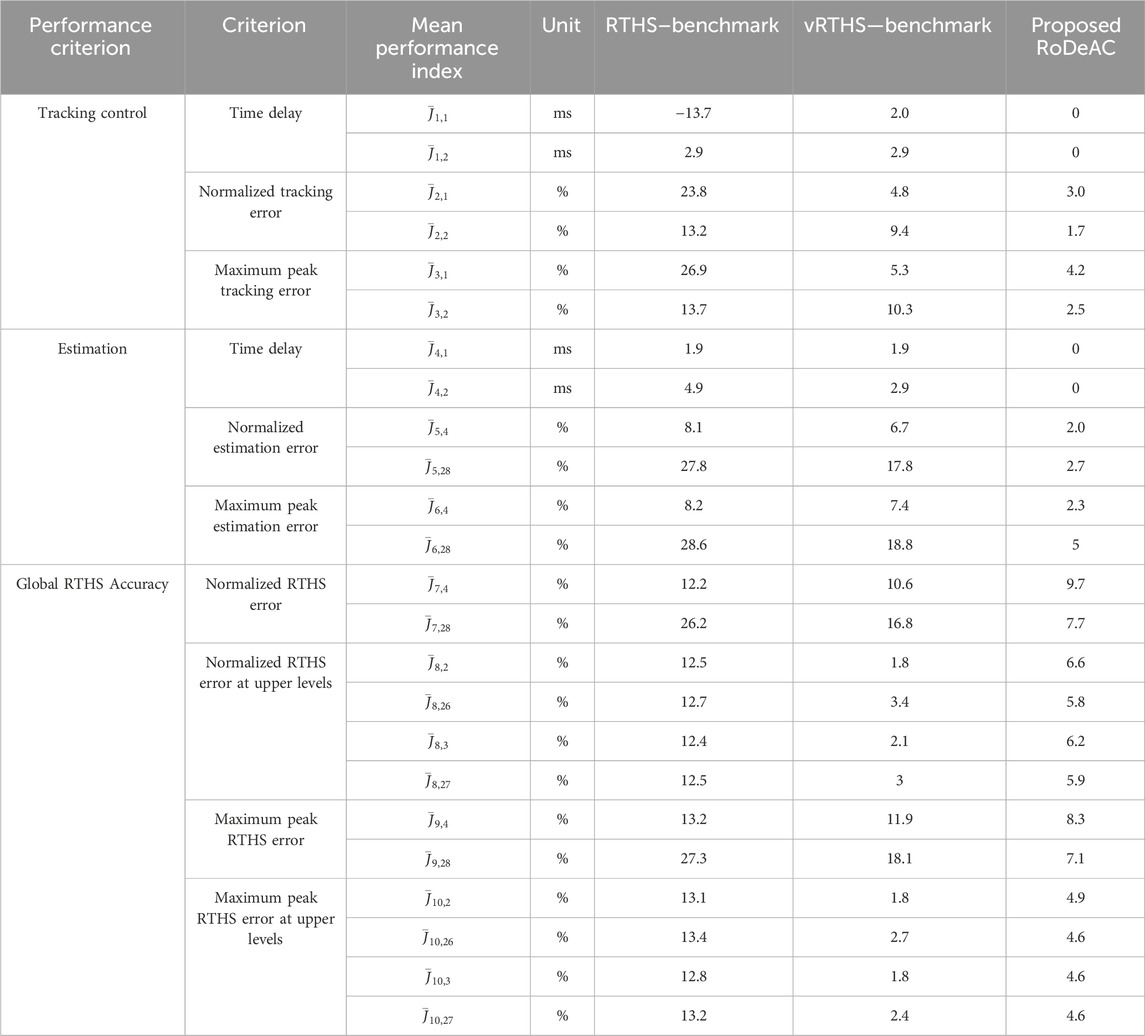
Table 2. Virtual maRTHS evaluation criteria (100 realizations).
The median value of the performance indices of 100 consecutive experiments using RoDeAC, along with the interquartile range, for the El Centro earthquake, scaled to 40% of the PGA intensity, and compared with 100 consecutive experiments with the benchmark controller, are plotted in Figure 17A. Tracking control and estimation indices show that RoDeAC has lower errors than the benchmark controller. For the global RTHS accuracy, the normalized and peak errors are lower at the controlled levels but slightly higher at the upper levels. Along with its high level of robustness, RoDeAC demonstrates excellent overall performance. More information on the performance comparison of the RoDeAC with the benchmark controller for other ground motions can be found in Appendix B of the Supplementary Material. Finally, Figure 17B summarizes the performance indices for the proposed RoDeAC, showing the controller’s stable and consistent behavior for the three chosen earthquakes and with 100 different perturbations of the control plant. In particular, the worst performance indices were obtained from the Morgan earthquake with 40% PGA.
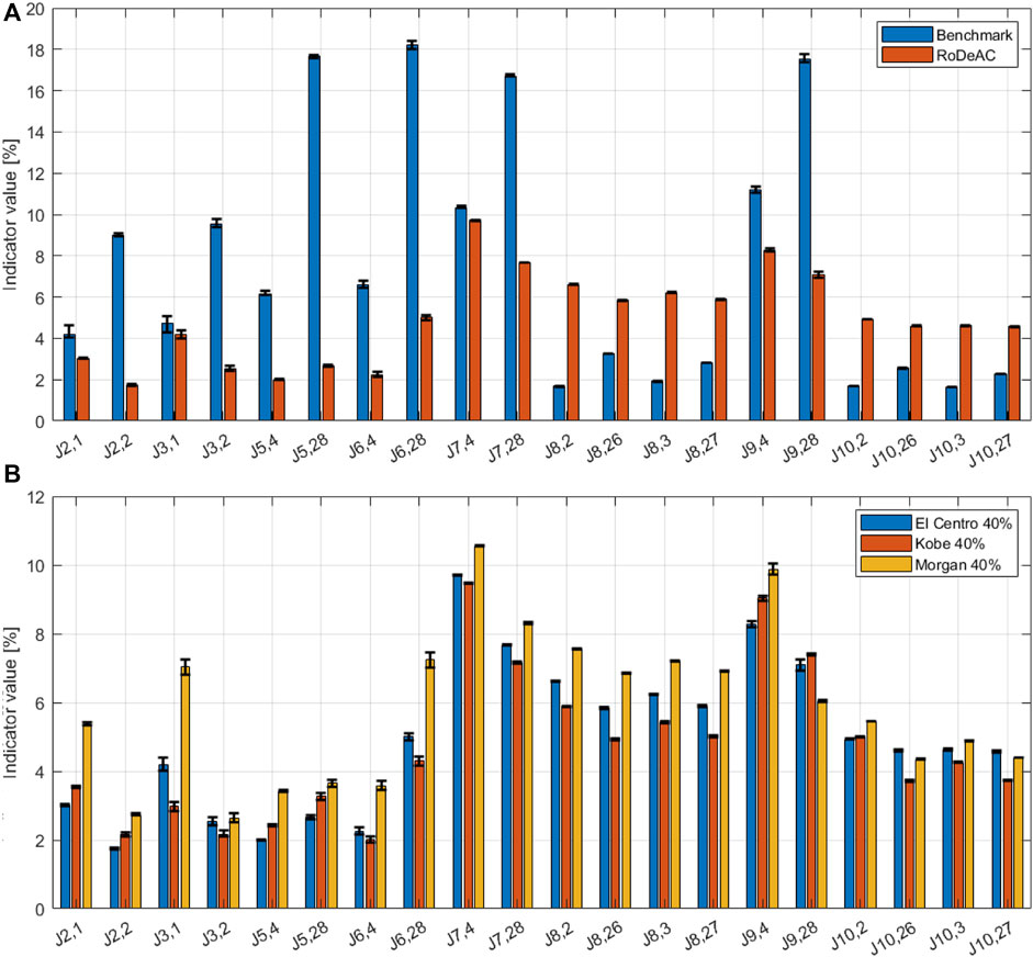
Figure 17. Comparison of evaluation criteria between benchmark and RoDeAC with 100 perturbed systems (median and interquartile range): (A) El Centro 40% PGA scaled and (B) summary of evaluation criteria for the three analyzed earthquakes.
On the other hand, the synchronization subspace plots (SSPs) of displacements comparing the benchmark and RoDeAC controllers are shown in Figure 18 for all three earthquakes as inputs of the systems scaled to 40% of the PGA intensity. This visualization allows us to directly compare the system’s synchronization, where a straight line with a 1:1 slope represents a perfect synchronization. The plots show that the best synchronization is achieved for the RoDeAC controller in all cases with thinner SSPs. Nevertheless, the Cartesian SSPs show slightly worse tracking performance compared with the actuator SSPs, especially for the rotation degree of freedom.
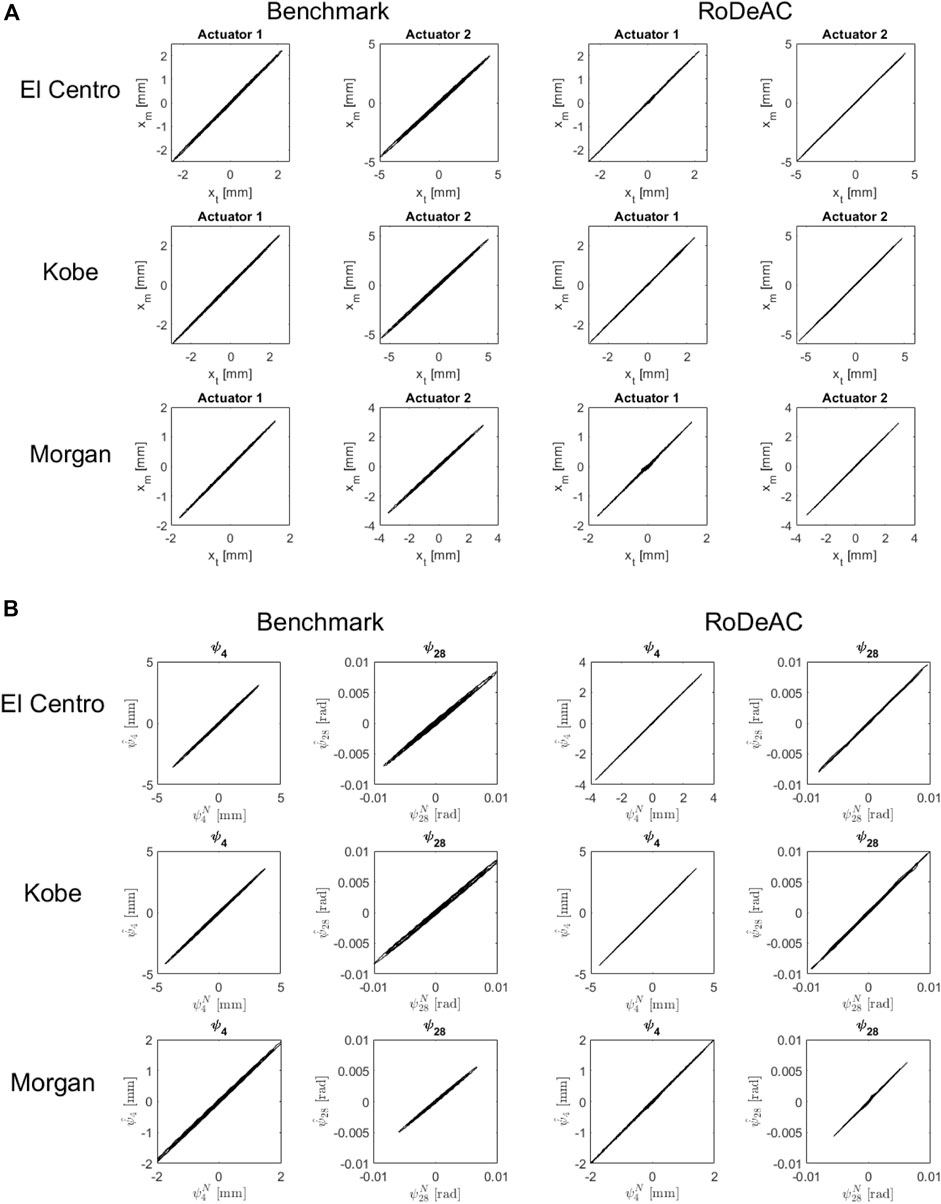
Figure 18. Synchronization subspace plots for benchmark and RoDeAC controllers (nominal plant): (A) actuator coordinates and (B) Cartesian coordinates
6 Conclusion
A robust decentralized adaptive compensator (RoDeAC) was proposed and examined through the next-generation multi-axial real-time hybrid simulation (maRTHS) benchmark problem. In particular, the reference structure corresponds to a three-story, three-bay planar frame where one central frame is the experimental substructure and the rest is the numerical substructure. Displacement and rotation are commanded as target signals at the interface between substructures. Two almost identical actuators are utilized to impose the numerical response; therefore, displacement and rotation are transformed into actuator coordinates to obtain one target signal for each actuator. Then, a decentralized recursive least squares adaptive compensator is employed over the multi-actuator loading assembly. In the virtual implementation, the actuator dynamics are modeled as a family of frequency response function (FRF) models with random parameters to consider actual uncertainty properly during experimental testing. The simulations show excellent tracking results for maRTHS tests and proper robustness even against the uncertainties in the modeled control plant for the three considered earthquake ground motions. It should be noticed that the relatively easy calibration algorithm required for the RoDeAC enables faster implementation of a compensation algorithm, even for more complex problems with a higher number of actuators. Future studies will consider the effect of sampling time and size on the RLS adaptive compensator, and experimental validation of this framework will be conducted on a physical testbed.
Data availability statement
The models and datasets presented in this study can be found in the following online repository: https://github.com/FermandoisLab/maRTHS-bmk-RoDeAC.
Author contributions
MQ: writing–review and editing, writing–original draft, visualization, validation, software, methodology, investigation, formal analysis, data curation, and conceptualization. CG: writing–review and editing, validation, software, resources, methodology, and conceptualization. GF: writing–review and editing, validation, supervision, resources, methodology, and conceptualization.
Funding
The author(s) declare that financial support was received for the research, authorship, and/or publication of this article. This research was supported by Agencia Nacional de Investigación y Desarrollo (ANID, Chile) through the Fondecyt Iniciacion Grant No. 11190774.
Conflict of interest
The authors declare that the research was conducted in the absence of any commercial or financial relationships that could be construed as a potential conflict of interest.
Publisher’s note
All claims expressed in this article are solely those of the authors and do not necessarily represent those of their affiliated organizations, or those of the publisher, the editors, and the reviewers. Any product that may be evaluated in this article, or claim that may be made by its manufacturer, is not guaranteed or endorsed by the publisher.
Supplementary material
The Supplementary Material for this article can be found online at: https://www.frontiersin.org/articles/10.3389/fbuil.2024.1394952/full#supplementary-material
References
Asai, T., Chang, C. M., Phillips, B. M., and Spencer, B. F. (2013). Real-time hybrid simulation of a smart outrigger damping system for high-rise buildings. Eng. Struct. 57, 177–188. doi:10.1016/j.engstruct.2013.09.016
Botelho, R. M., and Christenson, R. E. (2014). Mathematical framework for real-time hybrid substructuring of marine structural systems. Conf. Proc. Soc. Exp. Mech. Ser. 4 (February), 175–185. doi:10.1007/978-3-319-04546-7_21
Carrion, J. E., and Spencer, B. F. (2007). Model-based strategies for real-time hybrid testing. Newmark Structural Engineering Laboratory Report Series No. 006. Urbana, IL: Department of Civil and Environmental Engineering, University of Illinois at Urbana-Champaign. URL: http://hdl.handle.net/2142/3629.
Chae, Y., Kazemibidokhti, K., and Ricles, J. M. (2013). Adaptive time series compensator for delay compensation of servo-hydraulic systems for real-time hybrid simulation. Earthq. Eng. Struct. Dyn. 42, 1967–1715. doi:10.1002/eqe.2294
Chen, C., and Ricles, J. M. (2010). Tracking error-based servohydraulic actuator adaptive compensation for real-time hybrid simulation. J. Struct. Eng. 136 (4), 432–440. doi:10.1061/(ASCE)ST.1943-541X.0000124
Chen, P. C., Chang, C. M., Spencer, B. F., and Tsai, K. C. (2015). Adaptive model-based tracking control for real-time hybrid simulation. Bull. Earthq. Eng. 13 (6), 1633–1653. doi:10.1007/s10518-014-9681-2
Condori, J. W., Salmeron, M., Patino, E., Montoya, H., Dyke, S. J., Silva, C. S., et al. (2023). Experimental benchmark control problem for multi-axial real-time hybrid simulation. Front. Built Environ. 9. doi:10.3389/fbuil.2023.1270996
Dermitzakis, S. N., and Mahin, S. A. (1985). Development of substructuring techniques for on-line computer controlled seismic performance testing. Report No. UCB/EERC-85/04. Berkeley, California: Earthquake Engineering Research Center, University of California.
Fermandois, G. A., and Spencer, B. F. (2017). Model-based framework for multi-axial real-time hybrid simulation testing. Earthq. Eng. Eng. Vib. 16 (4), 671–691. doi:10.1007/s11803-017-0407-8
Galmez, C., and Fermandois, G. (2022). “Recent developments on robust adaptive compensation in multi-axial real-time hybrid simulation,” in Proceedings of the 8th World Conference on Structural Control and Health Monitoring, Orlando, FL, 5-8 June, 2022.
Ghaffary, A., and Mohammadi, R. K. (2019). Comprehensive nonlinear seismic performance assessment of MR damper controlled systems using virtual real-time hybrid simulation. Struct. Des. Tall Special Build. 28 (8), 1–18. doi:10.1002/tal.1606
Horiuchi, T., Inoue, M., Konno, T., and Namita, Y. (1999). Real-time hybrid experimental system with actuator delay compensation and its application to a piping system with energy absorber. Earthq. Eng. Struct. Dyn. 28 (10), 1121–1141. doi:10.1002/(SICI)1096-9845(199910)28:10<1121::AID-EQE858>3.0.CO;2-O
Horiuchi, T., Nakagawa, M., Sugano, M., and Konno, T. (1996). Development of a real-time hybrid experimental system with actuator delay compensation. Proc. of 11th World Conf. Earthquake Engineering, Acapulco, Mexico, June 23–28.
Najafi, A., Fermandois, G. A., Dyke, S. J., and Spencer, B. F. (2023). Hybrid simulation with multiple actuators: a state-of-the-art review. Eng. Struct. 276 (2022), 115284. doi:10.1016/j.engstruct.2022.115284
Najafi, A., Fermandois, G. A., and Spencer, B. F. (2020). Decoupled model-based real-time hybrid simulation with multi-axial load and boundary condition boxes. Eng. Struct. 219 (May), 110868. doi:10.1016/j.engstruct.2020.110868
Nakashima, M., Kato, H., and Takaoka, E. (1992). Development of real-time pseudo dynamic testing. Earthq. Eng. Struct. Dyn. 21 (1), 79–92. doi:10.1002/eqe.4290210106
Ning, X., Wang, Z., and Wu, B. (2020). Kalman filter-based adaptive delay compensation for benchmark problem in real-time hybrid simulation. Appl. Sci. 10 (20), 7101. doi:10.3390/app10207101
Palacio-Betancur, A., and Gutierrez Soto, M. (2019). Adaptive tracking control for real-time hybrid simulation of structures subjected to seismic loading. Mech. Syst. Signal Process. 134, 106345. doi:10.1016/j.ymssp.2019.106345
Phillips, B. M., and Spencer, B. F. (2012). Model-based framework for real-time dynamic structural performance evaluation. Newmark Structural Engineering Laboratory Report Series No. 031. University of Illinois at Urbana-Champaign 31 (August), 46–59. URL: http://hdl.handle.net/2142/33794.
Silva, C. E., Gomez, D., Amin, M., Dyke, S. J., and Spencer, B. F. (2020). Benchmark control problem for real-time hybrid simulation. Mech. Syst. Signal Process. 135, 106381. doi:10.1016/j.ymssp.2019.106381
Tao, J., and Mercan, O. (2019). A study on a benchmark control problem for real-time hybrid simulation with a tracking error-based adaptive compensator combined with a supplementary proportional-integral-derivative controller. Mech. Syst. Signal Process. 134, 106346. doi:10.1016/j.ymssp.2019.106346
Wang, Z., Guoshan, Xu, Qiang, Li, and Bin, Wu (2020). An adaptive delay compensation method based on a discrete system model for real-time hybrid simulation. Smart Struct. Syst. 25 (5), 569–580. doi:10.12989/sss.2020.25.5.569
Keywords: real-time hybrid simulation, multiple actuators, adaptive compensation, decentralized control, dynamic coupling, benchmark
Citation: Quiroz M, Gálmez C and Fermandois GA (2024) Robust decentralized adaptive compensation for the multi-axial real-time hybrid simulation benchmark. Front. Built Environ. 10:1394952. doi: 10.3389/fbuil.2024.1394952
Received: 02 March 2024; Accepted: 03 June 2024;
Published: 08 July 2024.
Edited by:
Eleni N. Chatzi, ETH Zürich, SwitzerlandReviewed by:
Giuseppe Abbiati, Aarhus University, DenmarkArturo Montoya, University of Texas at San Antonio, United States
Copyright © 2024 Quiroz, Gálmez and Fermandois. This is an open-access article distributed under the terms of the Creative Commons Attribution License (CC BY). The use, distribution or reproduction in other forums is permitted, provided the original author(s) and the copyright owner(s) are credited and that the original publication in this journal is cited, in accordance with accepted academic practice. No use, distribution or reproduction is permitted which does not comply with these terms.
*Correspondence: Gastón A. Fermandois, Z2FzdG9uLmZlcm1hbmRvaXNAdXNtLmNs