A simplified method for estimating bridge frequency effects considering train mass

The dynamic response of a railway bridge depends on several parameters; the primary parameter is the fundamental natural frequency of vibration of the bridge itself. It is considered a critical parameter of the bridge as the driving or the forcing frequencies arising from moving trains may coincide with the fundamental frequency of the bridge and initiate a resonant response amplifying the bridge load effects. This condition may adversely affect the stresses experienced on bridge members and, consequently, the remaining fatigue life of the structure. Because the train adds additional time-varying mass to the bridge, this introduces a time-varying change in the bridge’s fundamental natural frequency of vibration. As a result, train critical speeds will have a certain range depending on the train configuration. This article presents a simplified method using a power-law relationship to predict the frequency characteristics of a bridge as a function of the train-to-bridge mass ratio. The method is presented in a generalized form, which enables the frequency characteristics to be determined for any given combination of trains and simply supported bridges of short to medium span typically found on the UK rail network. The method is then demonstrated in a case study of a single-span, simply supported plate girder bridge. By considering the BS-5400 train traffic types, the proposed method is used to calculate bridge frequency effects, dynamic amplification, and train critical speed bandwidth for each train type. The simplicity of the proposed method, as it does not require any complex computational modeling, makes it an ideal and effective tool for the practicing engineer to carry out a quick and economical assessment of a bridge for any given train configuration.

1 Introduction

In the field of structural dynamics, the study of the dynamic response of railway bridges under a series of moving loads or sprung masses, which typically represent a train set, has received significant attention. Unlike road bridges, where loading is of a more random nature, for railway bridges, it is the periodic nature of the train axle loads from the consecutive passage of train wagons that give rise to unique frequency response spectrums. Under a resonant response condition, this can influence the magnitude of the bridge’s dynamic response and can, therefore, adversely affect the fatigue life of a bridge. With the on-going concern about many aging railway bridges, which is further exacerbated by the increase in the volume of rail traffic, axle loads, and train-operating speeds, this has become an area of increased research focus. For the bridge asset owner, the main objectives are to maintain the structural integrity and operational performance of the bridges and prolong their service life. Therefore, understanding the bridge–train interaction dynamic response and the parameters and conditions that can initiate a resonant response becomes extremely important as these can adversely affect fatigue. By knowing this information, an optimum train-operating and bridge maintenance regime can be implemented to prolong the life of the bridge.

The collapse of the Chester railway bridge in 1847 (Stokes, 1867) initiated research into the dynamics of railway bridges. Early investigations on railway bridge dynamics were performed using analytical and approximate methods (Yang et al., 2004a). Even during this early period, the importance of the bridge vibration frequency coinciding with the frequency of a series of impulse loads and how this affected the magnitude of the impact load was becoming clear (Robinson, 1886). Kryloff (1905) first presented the classical solution for a beam subjected to a moving load. Thereafter, much of the early assessment of bridge dynamic effects concentrated on the development of impact equations. Bridges in these early studies were simply represented as uniform beams, while the trains were represented as a series of moving loads that neglected any of the sprung masses. Using both moving load and moving mass type models on a simple beam, Timoshenko (1922) produced several studies using a moving load or pulsating force acting on the beam and proposed approximate solutions to the problem. Other researchers carried out similar studies during this period, such as those by Inglis (1934) and Lowan (1935). Inglis’s theoretical and experimental work paved the way for further development of the subject area, particularly the effects of impact on the vibration of railway bridges. Three of the most significant works in this area were carried out by Looney (1944), who introduced impact allowance factors into bridge design codes. These early models provided a means, using both analytical and numerical methods, by which the key parameters influencing bridge response could be investigated.

In the last few decades, the most comprehensive treatment of the subject of railway bridge dynamics has been provided by Frýba (1999) and Yang et al. (2004a). Yang et al. (2004b) provided a broad and systematic coverage of the interaction of the train with the bridge, particularly focusing on the vibration problems encountered in high-speed railway bridges. With the advent of modern computing, more complex train–bridge interaction models have evolved where the dynamics of the train and tracks are now introduced as a complete coupled system (Kwark et al., 2004; Yang et al., 2005; Dinh et al., 2009; Liu et al., 2009; Majka et al., 2009). The main focus of these models was to investigate how track irregularity and the dynamic interaction of the train affected the response of the bridge. In current bridge assessment codes, such as the UK railway bridge assessment code NR/GN/CIV/025 (2006), bridge dynamic effects are captured by calculating a dynamic amplification factor (DAF). The DAF is simply the ratio between the dynamic and static response and is calculated based on train speed, bridge natural frequency, and span lengths. The DAF provides a means by which dynamic effects, particularly when considering fatigue, can be accounted for in a quasi-static analysis. The methodology by which the DAF is calculated evolved though empirical means from the results of field tests and analytical studies. With modern high-speed trains and heavier train loads, the accuracy of the DAFs suggested in codes has been the subject of extensive research. Train–bridge interaction models, including coupled trains, have also been used to investigate bridge dynamic response to establish more accurate DAF values (Kwark et al., 2004; Karoumi et al., 2005; Majka and Hartnett, 2009; Wiberg, 2009; Hamidi and Danshoo, 2010; Imam and Yahya, 2014). These models are generally complex, requiring advanced finite element (FE) analysis or numerical models. Some of the latest works on train–bridge dynamic interaction modeling, involving the interaction of the moving mass with the bridge, require the solution of systems of equations involving large numbers of degrees of freedom with numerical methods (Koç, 2021; Koç and Esen, 2021; Koç et al., 2021). Kohl et al. (2023) provide one of the latest investigations into vehicle–bridge dynamic interaction effects using a 2D six degrees-of-freedom multi-body model (MBM).

The dynamic response of a bridge can be affected by multiple factors, including the train configuration, train mass, and speed. The primary flexural modes of vibrations are caused by the “driving frequencies,” which depend on the time that a train takes to cross the bridge, and the “dominant frequencies” associated with the repetitive axle loads (Yang and Lin, 2005; Ribes-Llario et al., 2016). These two parameters have been studied by various researchers investigating additional aspects of railway bridge dynamic response (Paultre et al., 1995; Frýba, 2001; Ju et al., 2009). Amplification of the bridge response can occur if a train speed is considered critical. Because the train mass can potentially affect the bridge’s natural frequency of vibration, the critical speed can also shift. This can also vary depending on the magnitude and position of the train mass on the bridge (Lu et al., 2012). Whether the bridge response is significantly affected depends on two parameters: the ratio of the bridge’s natural frequency to the frequency of the sprung mass of the train and the ratio of the bridge mass to that of the train (Doménech et al., 2012). These also determine whether a moving load model (MLM) or a multi-body model (MBM) is required to accurately capture the bridge dynamic response. For high values of the frequency ratio (bridge/train), the train–bridge interaction is not significant as both systems behave as though they are not dynamically coupled (Doménech et al., 2012). In this case, the MLM model is sufficient to model the train–bridge interaction. For lower frequency ratios and where the bridge–train mass ratio is low, which can be the case for light bridges, an MBM model is recommended (Doménech et al., 2012).

Much research provides an understanding of the frequency variation of bridges under moving trains (Li et al., 2003; Auersch, 2005; Ju et al., 2009; Xia et al., 2014; Bisadi et al., 2015). These studies explain the variation of the bridge’s natural frequency of vibration considering the train mass. Milne (2017) provides an understanding of the properties of train load frequencies considering the effects of vehicle geometry, bogie, and axle spacing. A study of critical train speeds and resonance cancellation effects is provided by Mao and Lu (2013). The general method introduced by Mao and Lu (2013) utilizes the classical beam theory to establish a means by which the reduction in the bridge’s fundamental frequency could be accounted for as a result of the train mass. Their work introduced a Z-factor that provides a measure of the severity of the resonance effect. An effective frequency ratio was also established to account for the reduction in frequency due to train mass. The study provided a means of identifying the critical train speeds that could cause the most serious resonance effects. This could potentially be used to control train speeds for existing bridges to minimize or eliminate the effects of resonance.

More recent studies have helped to identify the primary bridge frequencies and demonstrate that these are caused by the “driving frequencies” (Yang and Lin, 2005; Ribes-Llario et al., 2016). Other frequencies, termed the “dominant frequencies,” were identified as a result of the repeated loads and the time interval between consecutive carriages (Paultre et al., 1995; Frýba, 2001; Yang and Lin, 2005; Ju et al., 2009; Ribes-Llario et al., 2016). While numerous studies are available on critical train speeds, resonance effects, and their impact on bridge response, there is a lack of simplified methods that can provide a quick initial prediction of these effects. For the practicing engineer, a simplified analytical method by which trains could be accounted for when assessing bridge dynamic response and identifying critical train speeds would be beneficial. This would be particularly useful when considering standard trains, such as those available in the BS-5400 bridge assessment code, which are typically used in railway bridge fatigue assessments to quantify dynamic effects on fatigue damage accumulation rates on bridge members.

The complex models available in the literature, however, do not provide a closed-form solution and require considerable time and computational effort to analyze. The fact that MBM models require considerable computational effort compared to MLMs is acknowledged by Kohl et al. (2023). Furthermore, the parameters required for a MBM are generally not available in the public domain. Therefore, in practice, the MLMs still provide valuable and efficient means by which bridge dynamic response effects can be investigated. The MLMs can be used where there are negligible dynamic coupling effects between the train and bridge. This depends on the ratio of the natural frequency of vibration of the train suspension to that of the bridge. In a recent publication by Hora et al. (2023), the validity of the MLM approach was compared against a moving mass model (MMM) without considering the suspension system. The authors showed that both MLMs and MMMs gave the same displacement time responses for mass ratios less than 1.0. They concluded that the MMMs should be used when the moving mass becomes greater than the mass of the structure. In addition, MMMs showed a decrease in the resonant speeds as the mass ratio increased. In the current work of this article, the bridge structures analyzed with respect to the BS-5400 trains have mass ratios of less than 1.0.

MLMs can provide practical benefits for the practicing engineer who may be more interested in a first-level approximation for an initial and quick insight into the problem. They can be useful in establishing critical train speeds, and, most importantly, they could be used to assess the influence of dynamic effects on bridge fatigue relatively quickly for given train types, configurations, and speeds. A first-level assessment could help identify whether a more detailed assessment is needed, such as using an MBM approach. Researchers continue to study and identify parameters that can govern bridge dynamic response and resonance effects using both moving load and moving mass models (Li and Su, 1999; Yau, 2001; Garinei and Risitano, 2008; Martinez-Rodrigo et al., 2010). The work described in this article provides a general analytical method utilizing a power-law relationship to determine the reduction in a bridge’s natural frequency and the reduction in critical train speeds using a quasi-static-based analysis. This work enables a bridge frequency adjustment factor to be easily incorporated into the closed-form solution to the moving load problem provided by Frýba (1999). The methodology is based on the MLM but could be extended to include more complex MBMs, as proposed by Koç (2021) and Kohl et al. (2023), as well as for other types of bridge–train interaction problems.

2 Bridge model

The dynamic moving load models used in this study are based on the Euler–Bernoulli beam (EBB) theory as formulated by Frýba (2001) and a quasi-static moving load model using general beam deflection equations for a simply supported beam. The representation of the bridge response under a series of moving loads and the idealized form of the train loads for the EBB dynamic and quasi-static models are depicted in Figure 1 for a typical train. The model is implemented within MATLAB, and the dynamic response results are compared with the quasi-static moving load model.

Figure 1

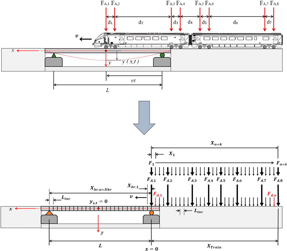
Figure 1. Bridge and train moving loads idealized for the mathematical model.

2.1 Euler–Bernoulli beam (EBB) model

The bridge response under a moving load can be solved using the classical Euler–Bernoulli beam theory, represented by Eq. 1, for a single moving load, P, traversing a beam (Svedholm, 2017).

${\displaystyle \sum _{i=1}^{\infty }}\left(EI\frac{{\partial }^4{\varphi }_i\left(x\right)}{\partial x^4}{q}_i\left(t\right)+\mu \frac{{\partial }^2{q}_i\left(t\right)}{\partial t^2}{\varphi }_i\left(x\right)+c\frac{\partial q_i\left(t\right)}{\partial t}{\varphi }_i\left(x\right)\right)=\delta \left(x-vt\right)P,(1)$

$EI$ Flexural rigidity of the beam with a constant moment of inertia,

${\varphi }_i\left(x\right)$ Linear combination of normal modes,

$q_i\left(t\right)$ Generalized coordinate of the n^th mode,

$x$ Length coordinate from the origin at the right hand of the beam,

$t$ Elapsed time from the instance at which the moving concentrated load P enters the beam,

$\mu$ Mass per unit length of the beam,

$c$ Equivalent coefficient of viscous damping of the beam,

$\delta$ Dirac delta function that describes a moving concentrated load,

$v$ Load traveling speed,

$P$ Moving concentrated load.

Eq. 1 describes the motion of a beam with a flexural rigidity, EI, and a uniformly distributed mass, $\mu$, along which the force, $P$, moves at constant velocity, $v$. The parameters on the right-hand side of Eq. 1 represent the motion of the constant force, which is described by the Dirac function $\delta \left(x\right)$ (Yang et al., 2004b). The function of the vertical deflection of the beam, $y\left(x,t\right)$, can be expressed as a product of two functions, the mode shape function (Eigen-function) ${\varphi }_i\left(x\right)$, and the function of the generalized coordinates $q_i\left(t\right)$. Eq. 1 forms the basis of the moving load model, which is then extended for a series of moving loads to the form given by Eq. 2 (Frýba, 1999; Yang et al., 2004a).

$EI\frac{{\partial }^{4}y\left(x,t\right)}{\partial x^4}+\mu \frac{{\partial }^{2}y\left(x,t\right)}{\partial t^2}+2\mu {\omega }_d\frac{\partial y\left(x,t\right)}{\partial t}={\displaystyle \sum _{n=1}^N}{\epsilon }_n\left(t\right)\delta \left(x-x_n\right)F_n,(2)$

$y\left(x,t\right)$ Vertical deflection of the bridge at position x and time t,

${\omega }_d$ Circular damped frequency of the bridge,

${\epsilon }_n\left(t\right)$ Describes the Heaviside unit step function for the arrival (turning on) and departure (turning off) of the n^th axle force, F_n,

$F_n$ Constant magnitude concentrated axle force,

$X_n$ Position of the n^th axle force, F_n, from the first axle,

$v$ Train constant speed,

$x_n=vt-X_n$ Position of the n^th axle force, F_n, from the bridge origin.

Eq. 2 is solved using the fundamental relationships of the Fourier sine integral transformation that presents the problem in the frequency domain. The Laplace–Carson integral transformation method is then applied to present the problem in the complex domain. The inversion of the Laplace–Carson transform presents the problem in real space, and the Fourier transform is then used to reduce the equation to the time domain. This method enables an analytical closed-form solution of Eq. 2. This method has been applied by Frýba (1999) to provide the closed-form solution, enabling the calculation of the vertical deflections of the bridge at any specific location x along the bridge as a function of time as given by Eq. 3. The equation expresses the forced vibration of the bridge due to the moving loads and the free transient damped vibrations after the train has left the bridge. The acceleration response of the bridge can be obtained by the double differentiation of Eq. 3.

$y\left(x,t\right)={\displaystyle \sum _{j=1}^{\infty }}{\displaystyle \sum _{n=1}^N}{y}_0{F}_{n}j\omega {\omega }_1^2\left[f\left(t-t_n\right)H\left(t-t_n\right)-{\left(-1\right)}^{j}f\left(t-T_n\right)H\left(t-T_n\right)\right]\mathit{sin}\frac{j\pi x,}{L}(3)$

$y_0$ Unit load deflection,

$L$ Bridge span,

$j$ j^th modal frequency (j = 1 for first vertical bending mode),

$\omega$ Forcing frequency,

${\omega }_1$ Circular natural frequency of vibration of the bridge (first vertical bending mode)

The solution is facilitated by introducing an incremental distance, $L_{inc}$, which must be a factor of the bridge span and train axle spacing and coupling distance dimensions. This value is based on the rightmost non-zero significant figure of any of the dimensions, and $L_{inc}$ must also be an integer $\ge 1$. With the first axle position on the bridge at time $t=0$, the complete train set length with the first axle as the origin is given by $X_{n=k}$, which is the position of the last axle, $k$, from the first. Dummy axle loads, $F_{d,1}\to F_{d,n}$, are introduced between each axle with zero values. These are positioned using the increment distance $L_{inc}$ to provide a series of equally spaced loads, $F_1\to F_k$, according to Figure 1. With reference to Figure 1, the time when the n^th axle force, $F_n$, enters the bridge is given by Eq. 4, whereas the time when it leaves the bridge is given by Eq. 5.

$t_n=\frac{X_n}{v},(4)$

$T_n=\frac{{L+X}_n}{v},(5)$

For the closed-form solution, Eq. 6 describes the Heaviside unit step function, $H\left(t\right)$, for the arrival (turning on) and departure (turning off) of the n^th axle force, $F_n$, and their time shifts $t-t_n$ and $t-T_n$, respectively.

${\epsilon }_n\left(t\right)=H\left(t-t_n\right)-H\left(t-T_n\right)H\left(t\right)=\left\{\begin{array}{c}0,t<0\\ 1,t\ge 0.\end{array}\right.(6)$

The parameter $f$ in Eq. 3 is a function of the inverse Laplace–Carson transformation, as given by Eq. 7. The first term expresses the response of the bridge due to the moving loads, and the second term is the transient response. The subscript j is the jth mode of vibration, where in this case, as we are only concerned with the bridge’s fundamental vertical bending mode of vibration, j = 1.

$f\left(t\right)=\frac{1}{{\omega }_j^{\prime }D}\left[\frac{{\omega }_j^{\prime }}{j\omega }\sin \left(j\omega t+\theta \right)+e^{-{\omega }_{d}t}\sin \left({\omega }_j^{\prime }t+\phi \right)\right].(7)$

The parameters of Eq. 7 are defined as follows:

${\omega }_j^{\prime }=\sqrt{{\omega }_j^2-{\omega }_d^2},(8)$

$D=\sqrt{{\left({\omega }_j^2-j^2{\omega }^2\right)}^2+4j^2{\omega }^2{\omega }_d^2,}(9)$

$\theta ={\tan }^{-1}\frac{-2j\omega {\omega }_d}{{\omega }_j^2-j^2{\omega }^2,}(10)$

$\phi ={\tan }^{-1}\frac{2{\omega }_d{\omega }_j^{\prime }}{{\omega }_d^2-{{\omega }^{\prime }}_j^2+j^2{\omega }^2,}(11)$

${\omega }_d=f_{\left(1\right)}\vartheta .(12)$

where ϑ is the logarithmic decrement of damping given by Eq. 13 (Frýba, 1999), and $f_{\left(1\right)}$ is the bridge’s fundamental vertical bending mode of vibration.

$\vartheta =\frac{1}{0.3L-0.0012L^2}.(13)$

Further details on the parameters and derivation of the equations can be found in Frýba (1999). The model equations were implemented and solved within MATLAB.

2.2 Quasi-static model

The mid-span bridge deflections are calculated using classical beam equations and employing the principle of superposition. Using this type of analysis, a DAF can be calculated using relevant codes of practice to account for the dynamic effects on deflections, bending moments, and stresses. This type of assessment is generally referred to as a quasi-static (Q-Static) analysis and cannot account for dynamic effects, such as a resonance response of the bridge, or the change in frequency of the bridge due to additional mass imposed on the bridge due to the train. However, as is shown in this article, the method can be used to obtain a general equation that can be used to predict the change in the frequency due to the train as a function of the unladen bridge resonant frequency and the train–bridge mass ratio. The method is also used to calculate a frequency reduction factor for each train–bridge configuration, which is then implemented in the EBB dynamic model to account for the vertical natural frequency reduction due to the mass of the train.

The quasi-static solution is facilitated by dividing the bridge span into equal increments based on the calculated $L_{inc}$ value, as discussed previously. Starting from position zero, the total number of bridge increments, $N_{br}$, is given using Eq. 14.

$N_{br}=1+\frac{L}{L_{inc}.}(14)$

Similarly, the total number of axles, $k$, including dummy axle loads, is given by Eq. 15, where $X_{Train}$ is the length of the train from the first to the last axle.

$k=1+\frac{X_{Train}}{L_{inc}}.(15)$

The deflection influence curve of the bridge at the mid-span, $a=0.5L$, is calculated using Eq 16, where $x$ is the position of the moving force given by $x=0:L_{inc}:L$, and $P$ is a unit load, which in this case is equal to 1 ton (9806.65 N).

$D_{br}=\begin{array}{c}\frac{Pa\left(L-x\right)\left(2Lx-x^2-a^2\right)}{6EIL}〈x\ge a〉\\ \frac{Px\left(L-a\right)\left(L^2-{\left(L-a\right)}^2-x^2\right)}{6EIL}〈x<a〉.\end{array}(16)$

For the series of axle loads crossing the bridge, the mid-span displacement is given by Eq. 17 using the principle of superposition.

${\delta }_{QStatic}={\displaystyle \sum _{j=1}^k}{\displaystyle \sum _{j+1}^{{j+N}_{br}}}{F}_j{D}_{br.}(17)$

To check the validity of the EBB dynamic and the quasi-static models, both models were run using two typical trains (S-T1 and EMU-T2) on two case study bridges (Bridges 1 and 2, respectively, see Table 1), which represent typical short- to medium-span railway bridges found on the UK rail network. The speed of the EBB dynamic model was set to 1 km/h to minimize any dynamic effects. The displacement response results are presented in Supplementary Figure S1, which shows that both models produce the same response results.

Table 1

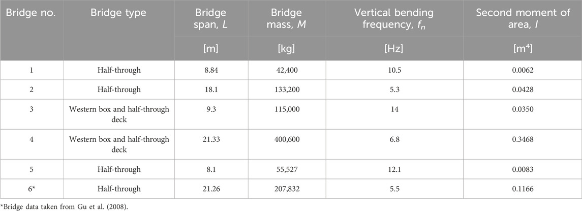
Table 1. Case study of plate girder bridges (Gaillard, 2003).

3 Case study bridges

To investigate the effect of train mass on the bridge resonant frequency, a range of plate girder bridges that are common on the UK rail network is considered. These bridges represent medium- and short-span bridges whose fundamental vertical bending mode resonant frequency varies between 5 Hz and 14 Hz. Table 1 lists the case study bridges and provides their key design parameters used in this assessment. Bridges 1 to 5 have been obtained from Gaillard (2003), while Bridge 6 has been obtained from Gu et al. (2008). Young’s modulus, E, was assumed to be equal to 210 GPa for all bridges.

The methodology employed for determining the effect of train mass on bridge frequency is demonstrated by arbitrarily using Bridge 2. This bridge is a half-though deck plate girder bridge with two main girders, as shown in Supplementary Figure S2. Transverse girders spaced at 508 mm are provided with concrete in-fill that supports a centrally located single track. For the EBB model, which is based on a uniform beam and considers the first bending mode of vibration, only flexural rigidity is required. Therefore, only Young’s modulus, E, and the second moment of area, I, are required for the analyses.

3.1 Finite element model of loaded beams

Because the case study bridges can be reasonably represented as uniform beams for predicting the fundamental vertical bending mode of vibration, a finite element analysis was performed to predict the change in frequency as a result of the additional mass imposed on the beam due to passing trains. Supplementary Figure S3 shows the FE models of each Bridges 1–6, which were developed using NX Siemens, represented as simply supported uniform beams with the flexural stiffness and mass properties as given in Table 1. Nodes were created to represent the axle spacings of train S-T1 with concentrated mass (CM) elements to which mass values were assigned. Train S-T1 represents Steel Train 1 as defined in BS-5400 (1980). The positions of the nodes were determined based on the maximum number of axles that could be positioned on the bridge to give a worst-case loading. Different positions of the train axles over the bridge simulating the train traveling across the bridge were considered, and the worst-case scenario was found to be when placing the train axles symmetrically about the mid-span of each beam.

The mass values represent axle masses that were incrementally changed from zero (unloaded beam) to a maximum value of 50,000 kg to study different M_w/M_b ratios. For each bridge model, eigenvalue analysis was performed to estimate the fundamental mode of vibration for each case. Table 2 shows the frequencies for the unloaded bridge and for an axle mass of 25,000 kg. The results in Table 2 are subsequently used to verify the frequency changes obtained using the generalized equations presented in this work.

Table 2

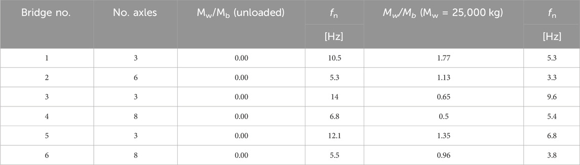
Table 2. FE model frequency analysis for case study bridges (loaded beam).

3.2 BS-5400 standard train mixes

For this study, the standard set of trains defined in BS-5400 (1980), shown in Supplementary Figure S4 and Supplementary Table S1, are included within the model, enabling the selection of any one type of train for analysis. Supplementary Table S1 also includes an additional hypothetical train with equally spaced axles, ESA-10. The train dimensions are as given in Supplementary Figure S4, and those that are used for the calculation of the wagon pass frequencies are in accordance with the train axle spacings as illustrated in Supplementary Figure S5 and Supplementary Table S2.

4 Bridge frequency analysis considering train mass

4.1 Bridge frequency and mass characterization

The assessment of bridge frequency considering train mass is performed following the steps outlined in the flow chart shown in Figure 2. The first step uses a quasi-static analysis to determine the mid-span displacement response for each train–bridge combination. The displacements are then used to calculate the mean bridge frequency, which represents the first vertical bending mode of the loaded bridge. For a simply supported beam, where the loading is mainly distributed uniformly, and the bridge is subjected to bending only, the fundament vertical bending mode natural frequency can be estimated using Eq. 12 (NR/GN/CIV/025, 2006) and EN1992-2, 2003.

$\begin{array}{cc}{f}_b=\frac{17.75}{\sqrt{{\delta }_o}}& {\delta }_o=mid-spandeflectionduetopermanentactions,\left(mm\right).\end{array}(18)$

Figure 2

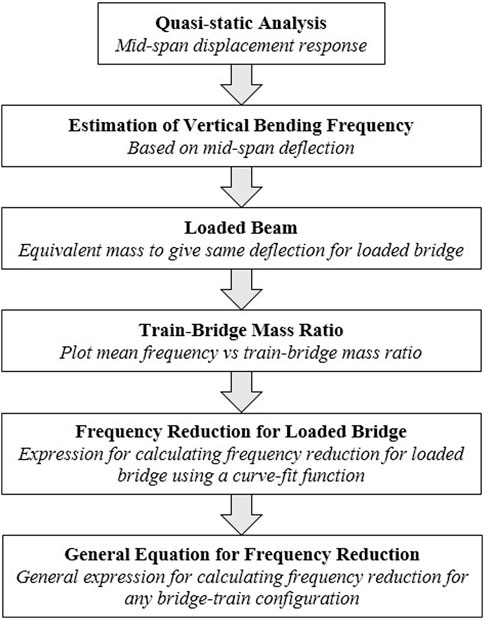
Figure 2. General process for considering frequency reduction for loaded bridges.

In this quasi-static assessment, the time history of mid-span deflection due to the moving train loads is accounted for by considering an additional permanent action leading to a total mid-span deflection of ${\delta }_o+y_t$. This enables the bridge’s fundamental vertical resonant frequency change to be obtained as a function of time. The effective bridge vertical bending mode resonant frequency is then taken as the mean frequency. Eq. 18 is therefore rewritten as follows:

$f_{b,t}=\frac{17.75}{\sqrt{{\delta }_o+y_t}}{y}_t=mid-spandeflectionasafunctionoftime,\left(mm\right).(19)$

It should be noted that using the lowest frequency would lead to the most undesirable scenario, resulting in the highest deflection. However, it is deemed that the mean frequency value is more reasonable to use to avoid overly conservative scenarios/cases. In a similar study, Mao and Lu (2013) also used a mean frequency value and specified this as being the effective natural frequency.

To account for the additional mass of the train on the bridge, the equivalent mass, $M_{w,t}$, is calculated as a function of mid-span deflection of $y_t$, Eq. 20. This is then used to calculate the mass ratio, M_w/M_b, for the given bridge–train configurations.

$M_{w,t}=\frac{{48EIy}_t}{g{L}^3}g=Gravitationalacceleration\left(\frac{m}{s^2}\right)y_t=mid-spandeflectionattimet\left(m\right).(20)$

The frequency variations for each train type are shown in Figure 3 and Figure 4. For train MF-T9, which is a mixed freight train, only wagons that lead to the longest periodic signal are considered. The results are also shown for a hypothetical train, Train ESA-10, which has equally spaced axles. The results for the frequency reduction due to the mass of the trains are given in Supplementary Table S3.

Figure 3

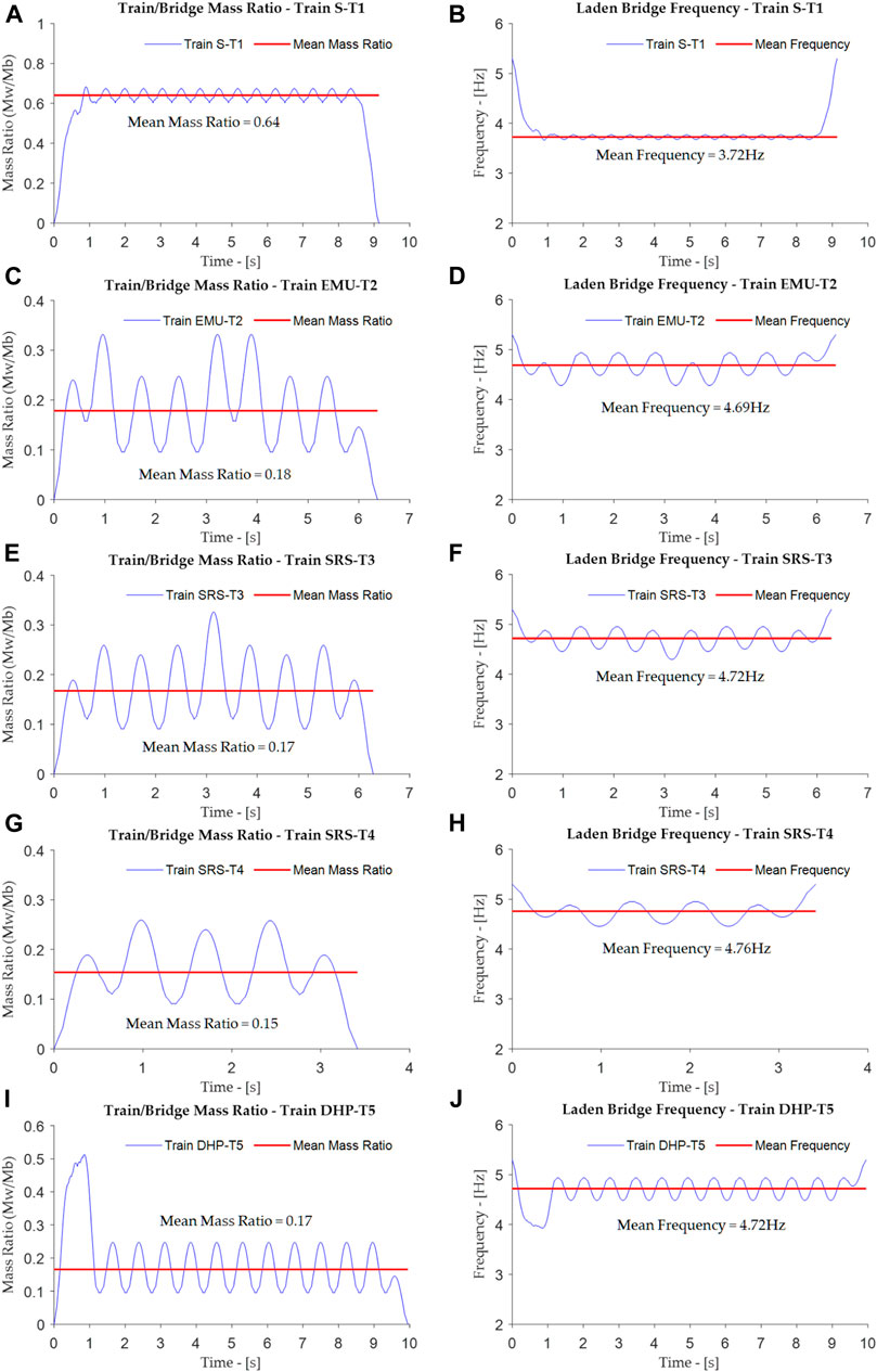
Figure 3. Train–bridge mass ratio and frequency: trains T1–T5.

Figure 4

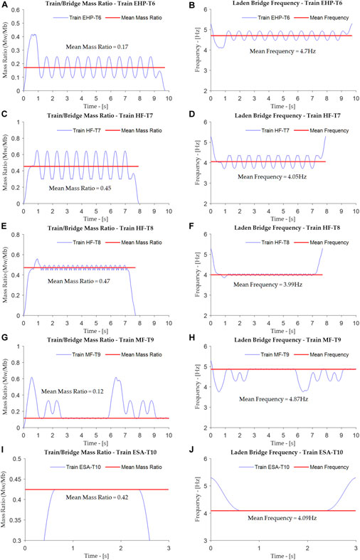
Figure 4. Train–bridge mass ratio and frequency: trains T6–T10.

4.2 Power-law approximation of bridge frequency considering train mass

By plotting the mean bridge frequency for each train as a function of the train–bridge mass ratio (M_W/M_b), it becomes apparent that a power law of the form $Y=A{X}^c$ (Roman, 2022) can describe the non-linear frequency–mass ratio relationship, as shown in Figure 5. To express the power-law relationship in the general form, as given by Eq. 21, the constant A and exponent c are determined by considering a range of bridges with different spans and resonant frequencies. Figure 5 shows that the first term in the equation represents the resonant frequency of the bridge. Therefore, the first expression in Eq. 21 is the fundamental bending frequency of vibration, f_n, of the bridge.

$f_{b,w}=f_n-A{\left(\frac{M_w}{M_b}\right)}^c.(21)$

Figure 5

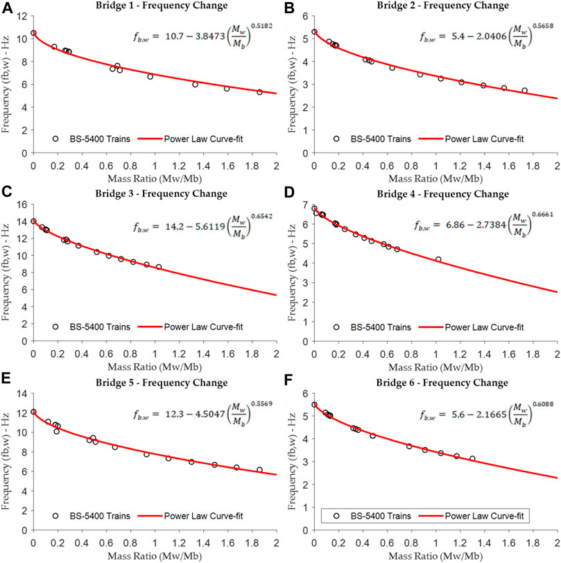
Figure 5. Frequency variation for train–bridge mass ratio.

The bridge frequency reduction factor, R_f, can also be obtained from Eq. 21. This is of particular use for the EBB model as it allows for the unloaded bridge fundamental resonant frequency to be adjusted for a particular bridge–train configuration without the need for any additional model amendments. The frequency reduction factor can be represented in the general form according to Eq. 22.

$R_f=1-\frac{A}{f_n}{\left(\frac{M_w}{M_b}\right)}^c.(22)$

The reduced frequency can be implemented in the EBB model, but this would require significantly more model code adjustment. This has been calculated separately, which is what is presented in the article, and the expressions have been simply included in the EBB model that calculates this reduction. As the EBB model already contains the databases for the bridges and the different BS-5400 trains, it is believed that this provides a simpler and more efficient means by which bridge frequency can be adjusted for the train mass.

The power-law constants and exponents for each bridge are shown in Table 3. The power-law parameters are plotted against the fundamental bridge vertical bending frequency in Figure 6. Both curves can be approximated to a linear curve from which the following expressions for the constant A and exponent c, Eqs 23, 24, respectively, can be derived. For simplicity, the exponent c can be approximated as equal to the intercept as the curve slope is effectively zero.

$A={0.3775f}_n+0.021.(23)$

$c={-0.0006f}_n+0.6006\approx 0.6.(24)$

Table 3

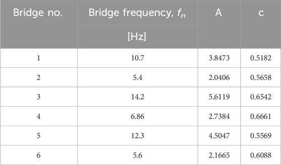
Table 3. Power-law constant and exponents.

Figure 6

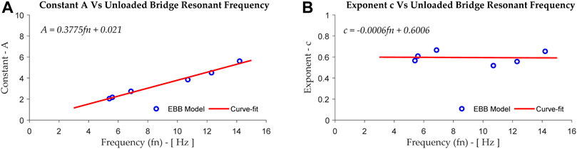
Figure 6. Constant A and exponent c as a function of frequency f_n.

Substituting Eqs 23, 24 into Eqs 21, 22 gives a general equation for the laden bridge resonant frequency, $f_{b,w}$, Eq. 25, and the frequency reduction factor, $R_f$, Eq. 26, for any given bridge where the fundamental bending frequency and train masses are known.

$f_{b,w}=f_n-\left(0.3775f_n+0.021\right){\left(\frac{M_w}{M_b}\right)}^{0.6}.(25)$

$R_f=1-\left(0.3775+\frac{0.021}{f_n}\right){\left(\frac{M_w}{M_b}\right)}^{0.6}.(26)$

Using Eqs 25, 26, the bridge frequency reduction and frequency reduction factors versus the train–bridge mass ratio are calculated for Bridges 1–6. Figure 7 shows that for low mass ratios (typically <0.3), the average reduction factor, $R_f$, is approximately 0.8. This means that a frequency reduction of 20% can be expected for bridges whose fundamental frequencies fall within the band 3–14 Hz.

Figure 7

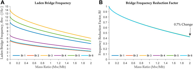
Figure 7. Laden bridge frequency reduction and reduction factor vs. mass ratio.

Figure 7B shows the frequency reduction factor does not change significantly between bridges. As can be seen in Figure 7B, the change in the reduction factor between the highest and lowest bridge frequencies is <1%. It can also be seen that the ratio of $\frac{0.021}{f_n}$ does not significantly contribute to the frequency reduction for the considered bridge group. For the lowest bridge frequency of 5.3 Hz (Bridge 2), the ratio is 0.00396, and for the highest bridge frequency of 14 Hz (Bridge 3), it is 0.0015.

4.3 General equation for bridge frequency considering train mass

As the bridge span is known, the additional mass on the bridge would need to be calculated for any given train. Therefore, it would be convenient to establish a train mass factor, T_mf, for the BS5400 trains, which would further simplify Eqs 25, 26. For the BS-5400 trains considered, the equivalent train mass is calculated using Eq. 14. The variation of the equivalent train mass for each train as a function of bridge span is shown in Figure 8. The curves allow the train mass factors, T_mf, to be calculated for each train type as a function of bridge span. The results are given in Table 4.

Figure 8

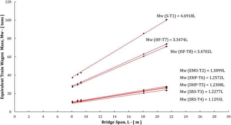
Figure 8. Equivalent train mass M_w vs. bridge span L.

Table 4

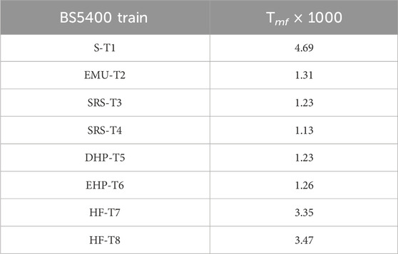
Table 4. Train mass factors, T_mf.

The train–bridge mass ratio, $M_w/M_b$, can be written using the train mass factors of Table 4, considering any of the BS-5400 trains, using Eq. 27. The term $\mu$ in this equation represents the uniformly distributed mass of the bridge.

$\frac{M_w}{M_b}=\frac{T_{mf}L}{\mu L}=\frac{T_{mf}}{\mu }.(27)$

The method and the frequency equations obtained can now be generalized in a more convenient form, offering the practicing engineer an efficient approach to assess bridge frequency under standard BS-5400 trains without the need for any complex dynamic modal numerical models. The method presented can also be extended to include other train types.

Using the general equation for calculating the fundamental bending frequency of a beam with a uniformly distributed mass, the frequency and the train–bridge mass terms in Eqs 25, 26 can now be replaced. Using Frýba (1999)’s definition of circular frequency at the j^th mode of vibration for a simply supported beam, as shown in Eq. 28, and substituting both Eqs 27, 28 into Eqs 25, 26, the following general equations for the BS-5400 trains can be derived to calculate the bridge resonance frequency and the frequency reduction factor (Eqs 29, 30, respectively). The equations are easily adaptable for any train type by establishing other train mass factors, T_mf, for non-BS-5400 trains.

$f_n=\frac{{\omega }_n}{2\pi }=\frac{\pi }{2}\sqrt{\frac{EI}{\mu L^4}.}(28)$

$f_{n,laden}=\frac{\pi }{2}\sqrt{\frac{EI}{\mu L^4}}-\left(\frac{151\pi }{800}\sqrt{\frac{EI}{\mu L^4}}+0.021\right){\left(\frac{T_{,mf}}{\mu }\right)}^{0.6}.(29)$

$R_f=1-\left(0.3775+\frac{0.021}{f_n}\right){\left(\frac{T_{,mf}}{\mu }\right)}^{0.6}.(30)$

In Section 4.2, it was shown that the ratio of $\frac{0.021}{f_n}$ does not significantly contribute to the frequency reduction for the considered bridge group. Therefore, for simplicity, this ratio can be ignored as it can be taken as zero. In addition, the remaining coefficient of 0.3775 can be rounded to 0.4, leading to a simplified equation for the frequency reduction factor, $R_f$, as given by Eq. 31.

$R_f=1-0.4{\left(\frac{T_{,mf}}{\mu }\right)}^{0.6}.(31)$

4.4 Comparison with finite element modal analysis of loaded beams

The Siemens NX FE models created in Section 2.1 for each Bridge 1–6 are used to calculate the frequency change for different train–bridge mass ratios, as summarized in Table 2. These results are now compared with those obtained using the methodology presented in the previous section. Comparisons are made for the following types of assessment against the FE model results:

- EBB dynamic model

- Frequency reduction equation based on a power-law curve-fit of the EBB dynamic model results

- Frequency reduction based on the general equation, Eq. 15

- Frequency reduction based on the general equation with train mass factor, $T_{,mf}$, Eq. 30

The laden bridge frequencies for each bridge are shown in Figure 9 for Bridges 1, 3, and 5 and Figure 10 for Bridges 2, 4, and 6. The results for Bridges 1, 3, and 5, which are considered short-span bridges (<10 m span), show a good correlation between each of the assessment methods; however, the results using the general equation start to diverge for the higher mass ratios. It is noteworthy that the higher mass ratios do not represent real train scenarios.

Figure 9

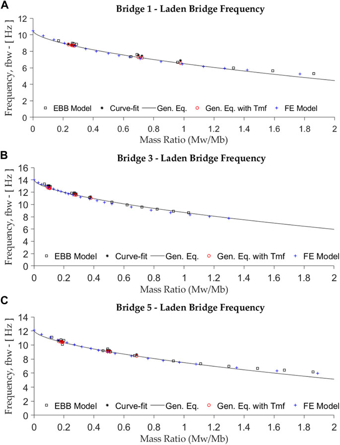
Figure 9. Laden bridge frequencies for BS5400 trains: Bridges 1, 3, and 5.

Figure 10

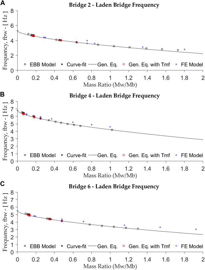
Figure 10. Laden bridge frequencies for BS5400 trains: Bridges 2, 4, and 6.

The same is true for Bridges 2, 4, and 6, which are considered medium-span bridges (10–25 m span), as shown in Figure 10. One reason for this is that the general equations have been derived based on the BS-5400 trains and do not extend to the higher mass ratios as in the case of the FE model assessment, which are hypothetical as they do not represent real trains.

The general Eq. 27 is also used to calculate the bridge frequency reduction factor for a given $M_w/M_b$ ratio. The frequency reduction curves for Bridges 1, 3, and 5 are shown in Figure 11A, and those for Bridges 2, 4, and 6 are shown in Figure 11B. These provide a convenient graphical means by which a bridge’s fundamental vertical bending mode resonant frequency can be approximated for a given mass ratio based on the two bridge groups considered in this assessment, short span (<10 m) and medium span (10–25 m).

Figure 11

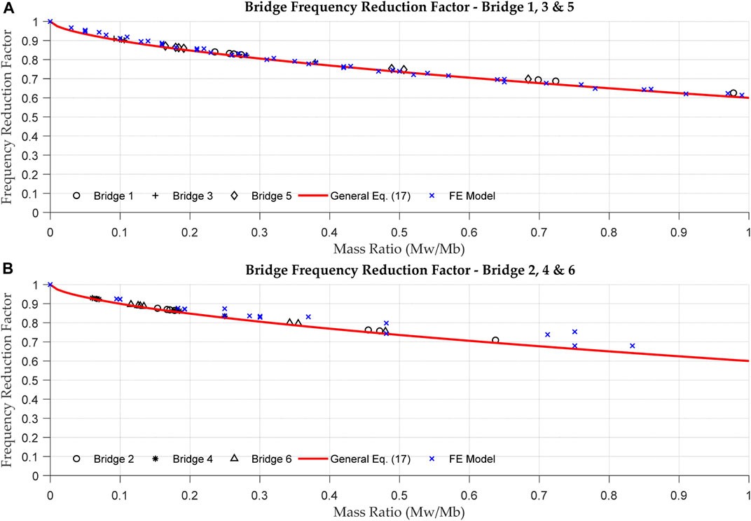
Figure 11. Frequency reduction factor for bridges based on BS-5400 trains.

4.5 Comparison with other studies

In this section, the results of the simplified model are compared with those of similar independent studies. Hora et al. (2023), using a multiple-moving mass and load model representing a train, show that for mass ratios < 1.0, both models produced similar bridge displacement responses. The result between the two started to diverge for mass ratios greater than 1.0, with the moving mass model producing higher bridge displacements (on the order of 12%) when the mass ratio reached 1.5. The authors show that the train’s critical speeds shift to the left for the moving mass analysis. The investigations conducted in this study show that the change in vertical resonant frequency is not greatly affected when the train–bridge mass ratios are <1.0, as can be seen in Figure 9 and Figure 10. The same divergence is generally seen when the train–bridge mass ratios are >1.0. As demonstrated in the Campbell diagrams in Figure 14 and Figure 15, showing the dynamic amplification factor against train speed, there is also a shift in DAF peaks between the unladen and laden cases. The DAF peaks represent a train’s critical speed, where the wagon pass frequency, or its multiples, coincides with the bridge’s vertical natural frequency of vibration.

In a recent publication, Kohl et al. (2023) analyzed a comprehensive set of trains and bridges using multi-body vehicle models. The main aim of the work is to establish the additional damping that could be incorporated into a moving load model to give the same maximum acceleration at the bridge mid-span obtained from a multi-body model. The results of the multi-body interaction model also showed a horizontal left shift and a reduction of the resonant speed of the ICE 2 and Eurostar trains due to the unsprung mass of the trains. To account for this reduction in the MLM model, the authors used an iterative method to determine the additional mass that could be added to the model to give the same effect. It is also worth noting that the suspension system frequencies are generally lower than the vertical bending mode of the bridge, which is typically >5 Hz, as is the case for the bridges considered in this work. This dynamically isolates the train body masses from the bridge, but as the authors note, this depends on the particular train–bridge configuration. Although this work is not directly comparable to the investigations in the current study, the general idea that an additional mass can be added to the MLM to account for the reduction in train critical speed is, in principle, the same.

Mao and Lu (2013) use the classical beam equation to represent a bridge with a moving vehicle to investigate the resonance phenomenon in the railway bridge response. In their study, the influence of the moving mass explicitly incorporates the coupled system dynamic properties. The study introduces a Z-factor that allows the prediction of the resonance effect but only if effective natural frequency is used in the calculation of resonance speeds. In their study, the effective natural frequency lies between the lowest natural frequency, when considering train mass, and the bridge’s fundamental vertical natural frequency of vibration. A similar methodology is incorporated in this study, where a mean train–bridge mass ratio and frequencies are used in the formulation of a set of generalized equations for predicting bridge resonance effects and train critical speeds. The main difference in this study is that actual assessment trains from BS-5400 are used as opposed to a hypothetical lumped mass model used by Mao and Lu (2013). Both studies present an approach by which bridge resonance effects and train critical speeds can be approximated. Both provide a means by which train critical speed bounds, accounting for train mass, can be approximated. The present study, which directly incorporates the BS-5400 trains, is considered to be of more practical relevance in real train–bridge assessments, particularly when considering fatigue.

Although more accurate and complex train–bridge multi-body system models are widely presented in the literature, these studies tend to look specifically at different areas of the train–bridge interaction, such as noise, wear, and passenger comfort. In such cases, modeling the train suspension systems, track irregularity, effects of sleepers, and even the ballast are necessary. However, whether this level of complexity is necessary when considering bridge fatigue effects is not a subject that has been adequately presented in the literature. Furthermore, many of the complex models presented in literature would not be easily understood or utilized by a practicing engineer, who, in most cases, is interested in a first approximation to see whether a potential problem exists for a particular train–bridge configuration. What this work aims to provide is a more efficient and practical means by which a practicing engineer can make a relatively simple assessment without resorting to complex models and assessment techniques.

5 Train critical speeds considering train mass

The train speed at which global bridge response reaches the maximum value is termed the “critical speed.” For a single moving load, the exciting frequency is given by the following:

${\mathrm{\Omega }}_n=\frac{n\pi v}{L}n=n^{th}modeofvibrationL=bridgelength\left[m\right]v=trainvelocity\left[\frac{m}{s}\right].(32)$

A resonant response of the bridge will occur when the ratio of moving load frequency of the excitation and the bridge natural frequency approaches 1, that is,

$\frac{{\mathrm{\Omega }}_n}{{\mathrm{\omega }}_n}=\frac{n\pi v}{{\mathrm{\omega }}_{n}L}{\omega }_n=bridgenaturalfrequencyofvibration\left[\frac{rad}{s}\right].(33)$

Therefore, the critical speed, without considering train mass, is given by the following equation.

$V_{cr}=2f_{1}L{f}_1=bridgefundamentalfrequencyofvibrationL=bridgelength\left[m\right].(34)$

For real trains, however, single moving loads do not exist, as each train will comprise a bogey with at least two or three axles. Typically, a train set will comprise a locomotive, or the engine carriage, and then a series of wagons. The number of wagons can be a single unit or multiples, and in some cases, mixed trains, as is the case for MF-T9 in Supplementary Table S1. In addition, there is a coupling distance between each connecting wagon, and similar to the axle spacing, this may vary between different train sets. To account for this, an equivalent wagon length is established and used to calculate train critical speeds.

Having established a general equation that gives a method for calculating the fundamental bending mode of a bridge for different types of trains, as defined in BS-5400 (1980), the equations can now be used to calculate train critical speeds for the bridges. The wagon pass frequency, $f_{wp}$, for a single train wagon can be calculated by considering the speed of the train and the length of the wagon, $L_{wagon}$, between the outer axles as follows (Mao and Lu, 2013):

$f_{wp}=\frac{5v}{18L_{wagon}}v=trainspeedin\frac{km}{h}.(35)$

As mentioned earlier, real trains typically have many wagons, which are coupled together with a coupling distance, $L_{we}$, between the adjoining wagons. Therefore, Eq. 35 is modified to account for the coupling effect; hence, the total length of the train, $L_{T,w}$, is given by:

$L_{T,w}=\left(L_w+L_{we}\right)N_w-L_{we.}(36)$

Normalizing Eq. 36, with respect to $N_w$, will lead to the equivalent wagon length, $L_{w,equivalent}$, which includes the coupling length and the contribution from the number of wagons.

$L_{w,equivalent}=L_w+L_{we}\left(1-\frac{1}{N_w}\right).(37)$

Substituting Eq. 37 for $L_{wagon}$ in Eq. 25 yields the wagon pass frequency, $f_{wp}$, for any train speed and wagon configurations:

$f_{wp}=\frac{5jv}{18L_{w,equivalent}}j=1,2,3,\dots ,nintegermultiples.(38)$

By rearranging Eq. 36 and representing the wagon pass frequency as a function of the natural bending frequency of the bridge, $f_n$, the critical train speed, $V_c$, can be calculated using Eq. 39.

$V_{c,unladen}=\frac{3.6L_{w,equivalent}}{j}{f}_{n.}(39)$

To account for the train mass on the bridge, the critical train speed (in km/h) for the laden bridge, $V_{c,laden}$, can be calculated by replacing unladen bridge frequency, $f_n$, with the laden bridge frequency $f_{b,laden}$, given in Eq. 30.

$V_{c,laden}=\frac{3.6L_{w,equivalent}}{j}{f}_{n,laden}.(40)$

Using Eqs 39, 40, the critical train speeds for the BS-5400 trains on each bridge are calculated for j = 1 (fundamental wagon pass frequency). Other integer multiples of the wagon pass frequency can simply be obtained by dividing the critical speed by different values of j accordingly. The verification of Eq. 32 is shown by the FFT analysis of the displacement response for Bridge 1 using trains S-T1, EMU-T2, and DHP-T5 running at the BS-5400 assessment speeds of 80 km/h, 145 km/h, and 160 km/h, respectively. Both modeling approaches, that is, the quasi-static and the dynamic model displacement response based on Eq. 3, are utilized here. The FFT results shown in Figures 12B, D, F identify the fundamental wagon pass frequency and how this is in agreement with that predicted by Eq. 33.

Figure 12

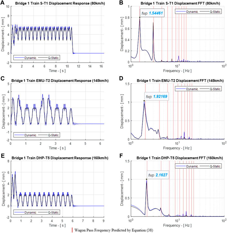
Figure 12. Bridge 1 response for trains S-T1, EMU-T2, and DHP-T5.

The results for the critical train speed that would cause a resonance response of the bridge for the laden and unladen cases are shown in Figure 12. As can be seen from the results, the critical speeds for both cases are well above the typical running speeds of the trains and the assessment speeds given in the bridge assessment code BS-5400 (1980), which are shown in Supplementary Table S5. The bar chart for the critical train speeds shown in Figure 13 presents the expected range of the variation of the critical speed for the different train types. As shorter bridge spans typically have higher vertical bending frequencies, the critical speeds are higher for Bridges 1, 3, and 5. Longer span bridges, spans >15 m, have lower bending frequencies, and these are shown to have lower critical train speeds for Bridges 2, 4, and 6.

Figure 13

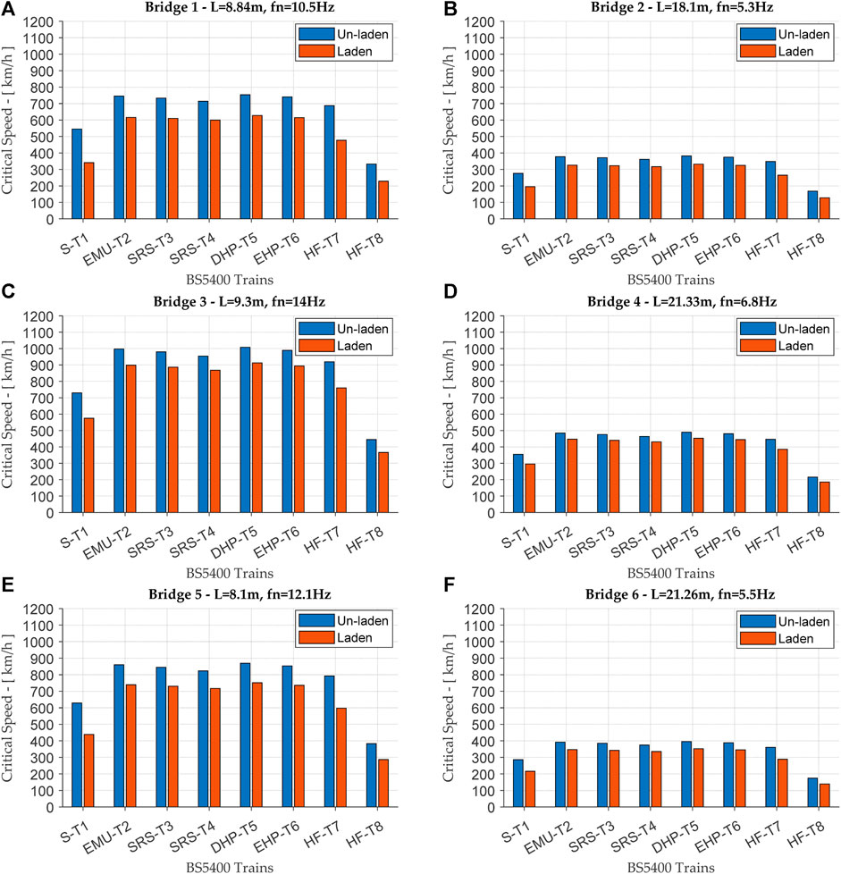
Figure 13. Critical speeds for bridges considering train mass.

Table 5 presents the critical speeds for trains EMU-T2 and HF-T8 for Bridges 1 and 2, which represent short- and medium-span bridges, respectively. These are calculated using Eqs 39, 40 for the unladen and laden conditions. The primary critical speeds when $j=1$ are all above the assessment speed for the EMU-T2 and HF-T8 trains, which are 145 km/h and 120 km/h, as given in Supplementary Table S5. However, this type of assessment cannot reveal any information on dynamic amplification or an indication of which multiples of the wagon pass frequency, $j{f}_{wp}$, will affect it. This information will be particularly important when considering fatigue damage, which is the subject of further investigation by the authors. To illustrate the effect on dynamic amplification, the EBB dynamic model, described in Section 2.1, is utilized to calculate dynamic amplification against train speed. This is then compared with the DAFs predicted by the bridge assessment code NR/GN/CIV/025 (2006). According to Eq. 41, dynamic amplification is defined in terms of deflection, where the peak values of $y_{\left(x,t\right),dynamic}$ and $y_{\left(x,t\right),static}$ displacement responses are used. The model accounts for the bridge’s fundamental vertical bending resonant frequency reduction due to the mass of the train using the method described in this work.

$DAF=\frac{y_{\left(x,t\right),dynamic}}{y_{\left(x,t,\right),static}}.(41)$

Table 5

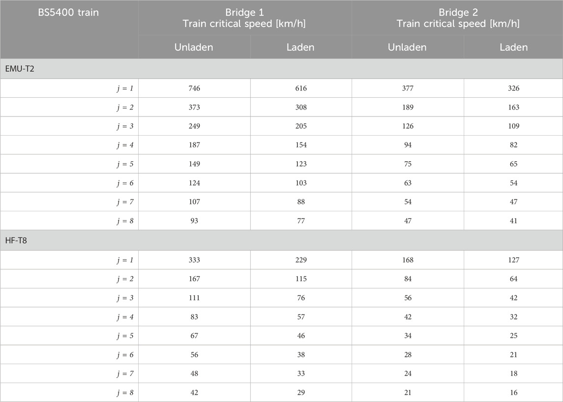
Table 5. Critical train speeds for Bridges 1 and 2.

A useful way of looking at vibration excitation at various train speeds is the Campbell diagram. This gives a bird’s eye view across the range of train speed and can help to identify where dynamic amplification increases due to the conditions of resonance. Therefore, the Campbell diagram is plotted using the displacement response results for Bridges 1 and 2 subjected to trains EMU-T2 and HF-T8. The results show that dynamic amplification that exceeds those based on the design/assessment codes can occur at other integer multiples of $j$. The Campbell diagram plots the multiples of the wagon pass frequency for each speed increment, 10 km/h in this case, and where the diagonal lines cross the bridge’s natural frequency of vibration line, indicating a possible critical speed at that multiple. Using the Campbell diagram plot, the multiples of $j$ at which dynamic amplification will occur become evident. These can then be compared with results given in Table 5, and those multiples of the wagon pass frequency, $j{f}_{wp}$, which affect dynamic amplification are thus highlighted in Table 5.

In Figure 14A (unladen), Bridge 1 with train EMU-T2, dynamic amplification occurs at a speed of approximately 110 km/h for the unladen case with a DAF of 1.24. There is also a minor peak at 50 km/h with a DAF of 1.16. The DAF at 110 km/h, which is within the operating speed of the train, represents an 11% increase from the code-based DAF. According to the calculated critical speed, 107 km/h, provided in Table 5, this occurs for $j=7$ or at $7f_{wp}$. For the laden condition, due to the reduction in the bridge resonant frequency, the critical speed drops to 90 km/h with no change in the magnitude of the DAF, Figure 14A (Laden).

Figure 14

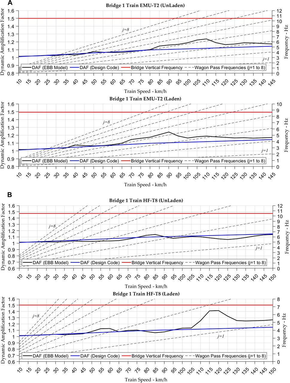
Figure 14. Dynamic amplification for Bridge 1 with trains EMU-T2 and HF-T8.

For train HF-T8 on Bridge 1, the response does not show any signs of a significant critical speed within the operating speed range of the train, Figure 14B. There is only a minor peak between 80 km/h and 85 km/h with a DAF of 1.14. However, for the laden case, a critical speed is shown to occur at a speed of 115 km/h with a DAF of 1.41, representing a 26% increase from the DAF from the assessment code. There is also a second minor peak between 55 km/h and 60 km/h with a DAF of 1.13, representing a 6% increase. Based on the calculated critical speed given in Table 5, these occur for $j=2,4$ or at $2f_{wp}$ and $4f_{wp}$.

Figure 15 shows the dynamic amplification for Bridge 2 with train EMU-T2. In Figure 15A (unladen), two minor peaks are evident at 55 km/h and between 125 km/h and 130 km/h for the unladen case, with DAF values of 1.1 and 1.14, respectively. These represent an increase of 6% and 3% from the DAF calculated based on the assessment code. For the laden case in Figure 15A (Laden), the critical speeds drop to 50 km/h and 110 km/h. According to Table 5, these minor critical speeds occur at 3 $f_{wp}$ and 7 $f_{wp}$.

Figure 15

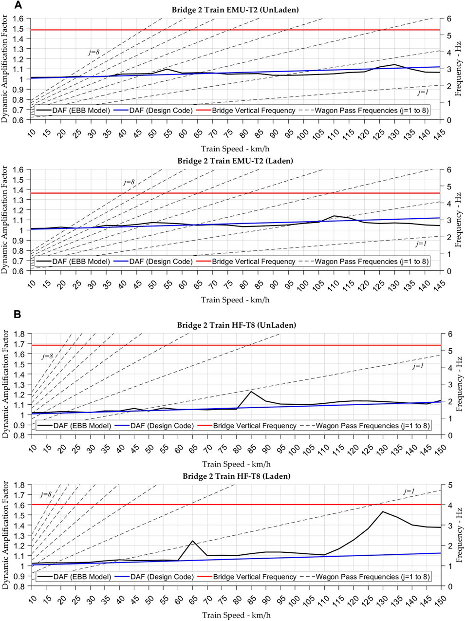
Figure 15. Dynamic amplification for Bridge 2 with trains EMU-T2 and HF-T.

As shown in Figure 15B, two significant critical speeds are identified for train HF-T8 on Bridge 2. For the unladen case, only a single critical speed is apparent within the speed range at 85 km/h with a DAF of 1.23, representing a 15% increase from the code-based DAF, Figure 15B (unladen). For the laden case, the most significant critical speed occurs at 130 km/h with a DAF of 1.53, representing a 38% increase from the assessment code DAF, Figure 15B (Laden). The critical speed at 85 km/h for the unladen case has now dropped to 65 km/h with a DAF of 1.25, representing a 19% increase. These critical speeds are shown to occur at 1 $f_{wp}$ and 2 $f_{wp}$, with the most significant at the primary wagon pass frequency, 1 $f_{wp}$.

6 Conclusion

This article has presented a simplified general method by which a bridge’s effective fundamental frequency can be calculated considering train mass. The assessment was made using the BS-5400 trains, but the methodology could be applied to other train types and bridges because the equations are also presented in a generalized form where only the train-to-bridge mass ratio needs to be known. The method was used to calculate a frequency reduction factor, which was then applied to the EBB dynamic model to assess the effect on critical speeds and dynamic amplification.

• For short-span bridges, typically with spans <10 m, the general equations presented show a reasonable correlation with those obtained from FE analysis.

• For longer spans, >15 m, the results also show a reasonable correlation for mass ratios <1.0. For higher mass ratios, typically for longer spans with more wagons on the bridge, results start to diverge between those predicted by the equation and the FE model. Therefore, care needs to be taken when considering longer-span bridges or higher $M_w/M_b$ ratios than 1.0.

• The unladen and laden critical speeds have been calculated for each train and bridge combination. By using the Campbell diagram, the effects on dynamic amplification for the two cases have been demonstrated on Bridges 1 and 2, representing short- and medium-span bridges, respectively. The results show that dynamic amplification can increase at other specific integer multiples of the wagon pass frequency, and these can fall within the operating speed range of the train. With the laden case, the amplitude of the dynamic amplification does not change, but as the vertical frequency of the bridge is reduced, the critical speeds are also reduced.

• The dynamic amplification plots using the Campbell diagram show that train HF-T8, which only has two axles as opposed to six for train EMU-T2, produces significantly higher DAFs. When compared with the DAF calculated with the bridge assessment code, this is 26% and 38% for Bridges 1 and 2, respectively.

• By showing the dynamic amplification variation with train speed, the Campbell diagram can be effective for the selection of optimum train speeds for a particular train/bridge combination.

The analysis mythology presented in this article has shown that simplified methods of assessment are able to provide valuable information, in particular, bridge dynamic amplification for different train–bridge configurations. As the method does not require complex computations or the use of finite element methods, the method is well-suited to give an initial indication of the performance of a bridge and help optimize train-operating speeds to minimize the effects of fatigue.

Data availability statement

The raw data supporting the conclusion of this article will be made available by the authors, without undue reservation.

Author contributions

AR: conceptualization, formal analysis, investigation, methodology, software, validation, visualization, writing–original draft, and writing–review and editing. BI: conceptualization, supervision, and writing–review and editing. DH: conceptualization, supervision, and writing–review and editing.

Funding

The author(s) declare that no financial support was received for the research, authorship, and/or publication of this article.

Conflict of interest

The authors declare that the research was conducted in the absence of any commercial or financial relationships that could be construed as a potential conflict of interest.

Publisher’s note

All claims expressed in this article are solely those of the authors and do not necessarily represent those of their affiliated organizations, or those of the publisher, the editors, and the reviewers. Any product that may be evaluated in this article, or claim that may be made by its manufacturer, is not guaranteed or endorsed by the publisher.

Supplementary material

The Supplementary Material for this article can be found online at: https://www.frontiersin.org/articles/10.3389/fbuil.2024.1382210/full#supplementary-material

References

Auersch, L. (2005). The excitation of ground vibration by rail traffic: theory of vehicle–track–soil interaction and measurements on high-speed lines. J.Sound Vib. 284, 103–132. doi:10.1016/j.jsv.2004.06.017

CrossRef Full Text | Google Scholar

Bisadi, M., Ma, Q. T., and Beskhyroun, S. (2015). “Evaluation of the dynamic amplification factor for railway bridges subjected to a series of moving mass,” in 5th ECCOMAS Thematic Conference on Computational Methods in Structural Dynamics and Earth-quake Engineering.

CrossRef Full Text | Google Scholar

BS-5400 (1980). Steel, concrete and composite bridges – Part 10: code of practice for fatigue.

Google Scholar

Dinh, V. N., Kim, K. D., and Warnitchai, P. (2009). Dynamic analysis of three-dimensional bridge-high speed train interactions using a wheel-rail contact model. Eng. Struct. 31 (12), 3090–3106. doi:10.1016/j.engstruct.2009.08.015

CrossRef Full Text | Google Scholar

Doménech, A., Museros, P., Nasarae, P., and Castillo-Linares, A. (2012). “Behavior of simply supported high-speed railway bridges at resonance: analysis of the influence of the vehicle model and simplified methods for dynamic analyses,” in Proceedings of ISMA2012-USD2012, 1057–1072.

Google Scholar

EN1992-2 (2003). Eurocode 2: design of concrete structures. Clause 6.4.4.

Google Scholar

Frýba, L. (1999). Vibration of solid structures under moving loads. 3. London: Thomas Telford.

Google Scholar

Frýba, L. (2001). A rough assessment of railway bridges for high speed trains. Eng. Struct. 23, 548–556. doi:10.1016/s0141-0296(00)00057-2

CrossRef Full Text | Google Scholar

Gaillard, C. S. (2003). Dynamic effects on structures of freight trains: project report. Report for the Rails Safety and Standards Board by Mott MacDonald.

Google Scholar

Garinei, A., and Risitano, G. (2008). Vibrations of railway bridges for high-speed trains under moving loads varying in time. Eng. Struct. 30 (3), 724–732. doi:10.1016/j.engstruct.2007.05.009

CrossRef Full Text | Google Scholar

Gu, G., Kapoor, A., and Lilley, D. M. (2008). Calculation of dynamic impact loads for railway bridges using a direct integration method. Proc. IMechE J. Rail Rapid Transit 222, 385–398. Part F. doi:10.1243/09544097jrrt189

CrossRef Full Text | Google Scholar

Hamidi, S. A., and Danshjoo, F. (2010). Determination of impact factor for steel railway bridges considering simultaneous effects of vehicle speed and axle distance to span length ratio. Eng. Struct. 32, 1369–1376. doi:10.1016/j.engstruct.2010.01.015

CrossRef Full Text | Google Scholar

Hora, R. C., Lima, S. S., and Santos, S. H. C. (2023). Moving mass/load speed influence on the structural dynamic response of a bridge. IBRACON Struct. Mater. J. 16 (6), e16601. doi:10.1590/s1983-41952023000600001

CrossRef Full Text | Google Scholar

Imam, B., and Yahya, N. F. (2014). “Dynamic amplification factors for existing truss bridges for the purposes of fatigue damage,” in Proc. 9th Int. Conf. Struct. Dyn., EURODYN 2014, Porto, Portugal, 30 June – 2 July 2014, 2311–9020. ISSN: ISBN: 978-972-752-165-4.

Google Scholar

Inglis, C. E. (1934). A mathematical treatise on vibration in railway bridges. Cambridge: The Cambridge University Press.

Google Scholar

Ju, S. H., Lin, H. T., and Huang, J. Y. (2009). Dominant frequencies of train-induced vibrations. J. Sound. Vib. 319, 247–259. doi:10.1016/j.jsv.2008.05.029

CrossRef Full Text | Google Scholar

Karoumi, R., Wiberg, J., and Liljencrantz, A. (2005). Monitoring traffic loads and dynamic effects using an instrumented railway bridge. Eng. Struct. 27 (12), 1813–1819. doi:10.1016/j.engstruct.2005.04.022

CrossRef Full Text | Google Scholar

Khol, A. M., Clement, K., Schneider, J., Firus, A., and Lombaert, G. (2023). An investigation of dynamic vehicle-interaction effects based on a comprehensive set of trains and bridges. Eng. Struct. 279, 1–13. doi:10.1016/j.engstruct.2022.115555

CrossRef Full Text | Google Scholar

Koç, M. A. (2021). Finite element and numerical vibration analysis of a Timoshenko and Euler-Bernoulli beams traversed by a moving high-speed train. J. Braz. Soc. Mech. Sci. Eng. 43, 165. doi:10.1007/s40430-021-02835-7

CrossRef Full Text | Google Scholar

Koç, M. A., and Esen, I. (2021). “Influence of train mass on vertical vibration behaviour of railway vehicle and bridge structure,” in 3rd International Symposium on Railway Systems Engineering (ISERSE’16), Karabuk, Turkey, 2021 October 13-15.

Google Scholar

Koç, M. A., Esen, I., Eroğlu, M., and Çay, Y. (2021). A new numerical method for analysing the interaction of a bridge structure and travelling cars due to multiple high-speed trains. Int. J. Heavy Veh. Syst. 28 (1), 79–109. doi:10.1504/ijhvs.2021.114415

CrossRef Full Text | Google Scholar

Kryloff, A. N. (1905). “Über die erzwungenen Schwingungen von gleichförmigen elastischen Stäben (On the forced oscillations of uniform elastic rods),” in Mathematische annalen. Mathematical collection of papers of the academy of sciences. Editor A. N. Kryloff (Peterburg: Matematischeskii sbornik Akademii Nauk), 61.

Google Scholar

Kwark, J. W., Choi, E. S., Kim, Y. J., Kim, B. S., and Kim, S. I. (2004). Dynamic behavior of two-span continuous concrete bridges under moving high-speed train. Comp. Struct. 82 (4), 463–474. doi:10.1016/s0045-7949(03)00054-3

CrossRef Full Text | Google Scholar

Li, J. Z., and Su, M. B. (1999). The resonant vibration for a simply supported girder bridge under high speed trains. J. Sound. Vib. 224 (5), 897–915. doi:10.1006/jsvi.1999.2226

CrossRef Full Text | Google Scholar

Li, J. Z., Su, M. B., and Fan, L. C. (2003). Natural frequency of railway girder bridges under vehicle loads. J. Bridge Eng. 8 (4), 199–203. doi:10.1061/(asce)1084-0702(2003)8:4(199)

CrossRef Full Text | Google Scholar

Liu, K., De Roeck, G., and Lombaert, G. (2009). The effect of dynamic train-bridge interaction on the bridge response during a train passage. J. Sound. Vibrat. 325 (1e2), 240–251. doi:10.1016/j.jsv.2009.03.021

CrossRef Full Text | Google Scholar

Looney, C. T. G. (1944). Impact on railway bridges, 352. University of Illinois bulletin, engineering experiment station bulletin series. 26th December 1944 No. 19.

Google Scholar

Lowan, A. N. (1935). On transverse oscillations of beams under the action of moving variable loads. Philos. Mag. Ser. 7 (127), 708–715. doi:10.1080/14786443508561407

CrossRef Full Text | Google Scholar

Lu, Y., Mao, L., and Woodward, P. (2012). Frequency characteristics of railway bridge response to moving trains with consideration of train mass. Eng. Struct. 42, 9–22. doi:10.1016/j.engstruct.2012.04.007

CrossRef Full Text | Google Scholar

Majka, M., and Hartnett, M. (2009). Dynamic response of bridges to moving trains: a study on effects of random track irregularities and bridge skewness. Comp. Struct 87 (19-20), 1233–1252. doi:10.1016/j.compstruc.2008.12.004

CrossRef Full Text | Google Scholar

Mao, L., and Lu, Y. (2013). Critical speed and resonance criteria of railway bridge response to moving trains. ASCE J. Bridge Eng. 18 (2), 131–141. doi:10.1061/(asce)be.1943-5592.0000336

CrossRef Full Text | Google Scholar

Martinez-Rodrigo, M. D., Lavado, J., and Museros, P. (2010). Dynamic performance of existing high-speed railway bridges under resonant conditions retrofitted with fluid viscous dampers. Eng. Struct. 32 (3), 808–828. doi:10.1016/j.engstruct.2009.12.008

CrossRef Full Text | Google Scholar

Milne, D. R. M., LePen, L. M., Thompson, D. J., and Powrie, W. (2017). Properties of train load frequencies and their applications. J.Sound Vib. 397, 123–140. doi:10.1016/j.jsv.2017.03.006

CrossRef Full Text | Google Scholar

NR/GN/CIV/025 (2006). The structural assessment of underbridges, network rail 2006.

Google Scholar

Paultre, P., Proulx, J., and Talbot, M. (1995). Dynamic testing procedures for highway bridges using traffic loads. J. Struct. Eng. 121 (2), 362–376. doi:10.1061/(asce)0733-9445(1995)121:2(362)

CrossRef Full Text | Google Scholar

Ribes-Llario, F., Zamorano-Martin, C., Morales-Ivorra, S., and Real-Herráiz, J. (2016). Study of vibrations in a short-span bridge under resonance conditions. JVE Int. Ltd. J. Vibroengineering 18 (5), 3186–3196. ISSN 1392-8716. doi:10.21595/jve.2016.16531

CrossRef Full Text | Google Scholar

Robinson, S. W. (1886). Bridge vibrations under passing train. New York: Railroad Gazette, 438–439.

Google Scholar

Roman, S.Bertolotti (2022). A master equation for power laws. J. R. Soc. Open Sci. 9, 1–10. The Royal Society. doi:10.1098/rsos.220531

CrossRef Full Text | Google Scholar

Stokes, G. G. (1867). Discussion of a differential equation related to the breaking of railway bridges. Trans. Camb. Phil. Soc. 8 (5).

Google Scholar

Svedholm, C. (2017). “Efficient modelling techniques for vibration analysis of railway bridges,” in Doctoral thesis in structural engineering and bridges, Stockholm, Sweden.

Google Scholar

Timoshenko, S. P. (1922). CV. On the forced vibrations of bridges. Lond. Edinb. Dublin Philosophical Mag. J. Sci. 43 (257), 1018–1019. doi:10.1080/14786442208633953

CrossRef Full Text | Google Scholar

Wiberg, J. (2009). Railway bridge response to passing trains – measurements and FE model updating. Stockholm, Sweden: KTH Architecture and the Built Environment. PhD Thesis.

Google Scholar

Xia, H., Li, L., Guo, W., and De-Roeck, G. (2014). Vibration resonance and cancellation of simply supported bridges under moving train loads. ASCE J. Eng. Mech. 140. doi:10.1061/(asce)em.1943-7889.0000714

CrossRef Full Text | Google Scholar

Yang, Y. B., and Lin, C. W. (2005). Vehicle-bridge interaction dynamics and potential applications. J. Sound. Vibrat. 284 (1-2), 205–226. doi:10.1016/j.jsv.2004.06.032

CrossRef Full Text | Google Scholar

Yang, Y. B., Yau, J. D., and Wu, Y. S. (2004a). Vehicle-bridge interaction dynamics. River Edge, NJ: World Scientific.

Google Scholar

Yang, Y. B., Yau, J. D., and Wu, Y. S. (2004b). Vehicle-bridge interaction dynamics – with applications to high-speed railways. Singapore: 1st ed. Wld. Sci. Pub. Co. Pte. Ltd, 1–530.

Google Scholar

Yau, J. D. (2001). Resonance of continuous bridges due to high speed trains. J. Mar. Sci. Technol. 9 (1), 14–20. doi:10.51400/2709-6998.2430

CrossRef Full Text | Google Scholar