Evaluation of stiffness and damping of a base-isolated building considering higher-order modes

Introduction: Structural health monitoring (SHM) is an effective method of understanding the seismic safety of seismic design models and the continued use of buildings after earthquakes. Various system identification methods applicable to SHM have been proposed; however, most target only superstructures. Their applicability for evaluating the soundness of foundations and soil structures should also be examined. In addition, evaluating high-order modes in addition to low-order modes is necessary to capture changes in the vibration characteristics of superstructures, foundations, and soil structures. However, the impact of considering higher-order modes on the identification results has not been sufficiently evaluated. This study aims to address these issues by clarifying the importance of considering higher-order modes and proposing a method that can contribute to improving the accuracy of future building health evaluation methods.

Methods: This study proposes a method of evaluating the stiffness and damping of a superstructure and dynamic soil spring considering low-order to high-order modes using the efficient transfer function fitting system for a base-isolated (BI) building. First, numerical experiments were performed to examine the accuracy of the proposed method in evaluating the stiffness and damping of each part when using acceleration data from limited observation points. Furthermore, this method was applied to an existing BI building subjected to the 2011 off the Pacific Coast of Tohoku Earthquake (2011 Tohoku Earthquake) to identify each parameter while considering higher-order modes. In addition, secular changes and the amplitude dependence of each structure were analyzed.

Results: The results showed that the stiffness and damping of the seismic isolation layer, superstructure, and dynamic soil spring were stable with little variation owing to aging; however, the influence of amplitude dependence was relatively large.

Conclusion: The significance of considering higher-order modes in evaluations of the soundness of foundations and soil structures was demonstrated. Moreover, the response characteristics of earthquakes recorded from 2007, before the 2011 Tohoku Earthquake, up to 2023 were accurately reproduced through numerical simulation by considering the amplitude dependence of the identified physical parameters based on the proposed identification framework.

1 Introduction

In Japan, where earthquakes occur frequently, structural health monitoring (SHM) is an important technology for building structures serving as business bases. SHM is a valuable tool for assessing the validity of the current seismic design models, improving seismic safety performance, rapidly determining the continuity of functions after earthquakes, and implementing effective measures for recovery. SHM has been applied to actual architecture and civil engineering structures (e.g., Limongelli and Çelebi, 2019). Efforts have primarily focused on developing SHM systems that detect changes in the stiffness and natural period of arbitrary layers and structural members of superstructures. In recent years, research has been actively conducted on damage-detection methods for each component by applying machine-learning technology (Byung et al., 2017; Zhang et al., 2023). SHM presents potential for further technological development. Considering earthquake damage to buildings in recent years, Kikitsu et al. (2017) reported that the continued use of some buildings was challenging owing to the damage to the foundation structure subjected to the 2011 off the Pacific Coast of Tohoku Earthquake (2011 Tohoku Earthquake) despite minor damages to superstructures. Therefore, future research should promote SHM that considers superstructures, foundations, and soil structures.

The SHM of structural foundations can be performed via direct and indirect monitoring. The former is conducted by embedding optical fibers or strain gauges in underground structures, such as piles, to detect structural damage (Hayashi et al., 2017). The latter is performed by detecting damage to pile foundations from changes in vibration characteristics based on sensor responses in the superstructure and footing (Hamamoto et al., 2010). Direct monitoring has high measurement accuracy; however, it is limited by the costs involved in installing the necessary devices into the piles and challenges in applying them to existing buildings. By contrast, indirect monitoring offers advantages in this regard. This study proposes an effective method for the SHM of a superstructure and indirect monitoring of structural foundations.

To date, various system identification methods applicable to SHM have been proposed. These methods can be broadly divided into two types. The methods of the first type employ modal parameter estimation techniques, such as the autoregressive exogenous (ARX) model and the subspace method (e.g., Safak, 1991; Verhaegen, 1993). Those of the second type employ a physical parameter identification techniques that directly estimate parameters, such as the shear stiffness and damping coefficient of a building, using a Kalman filter or particle filter (e.g., Hoshiya and Saito, 1984; Chen et al., 2005). Tojo and Nakai (2022) developed a modal parameter estimation technique based on the equation of motion of the sway-rocking (SR) model for the indirect monitoring of soil and structural foundations. However, as the physical parameters constitute a black box in this technique, estimating the damaged structural parts and damage degree is difficult. Methods of the second type enable the direct estimation of the physical parameters of buildings and can effectively determine damage locations. This method estimates the physical parameters of a numerical simulation model from measured vibration data. However, it is generally not possible to measure the responses of all stories of a building. To solve this problem, methods of estimating the health of building for all stories have been proposed using few acceleration sensor responses (e.g., Shinagawa and Mita, 2013; Suzuki and Mita, 2016; Shirzad-Ghaleroudkhani et al., 2017; Jabini et al., 2018). Moreover, Fujita and Takewaki (2018) proposed a method of estimating the responses of all stories based on non-simultaneous observations of each floor by moving the measurement device. In such methods, the vibration mode response or participation functions of all the stories must be estimated in advance. However, the full-story modal response cannot be estimated in advance for every building. Furthermore, these methods are obviously even more difficult to apply when evaluating underground foundation and soil structures.

Therefore, in this article, we propose a framework for identifying physical parameters using transfer functions to consider vibration mode characteristics efficiently up to high orders for application to the health monitoring of all stories of superstructures and indirect monitoring of foundations and soil structures. The novelties of this method are that identification is possible by using data from a limited number of observation points without estimating the modal responses of all stories in advance and that the ground response need not be used for indirect monitoring.

The proposed framework was validated by applying the modal iterative error correction (MIEC) method proposed by (Suzuki, 2018; Suzuki, 2019). The MIEC method is a general-purpose inverse analysis method used for input and output (I-O) systems. This method has been reported to estimate effectively the physical parameters of superstructures, including nonlinear characteristics, and the rotational input of a shaking table (Suzuki and Tojo, 2020; Uesaka et al., 2021a; Uesaka et al., 2021b). The proposed framework was applied to the SR model, and the physical parameters related to the stiffness and damping of superstructures and dynamic soil springs in the soil–structure interaction system were collectively identified. We believe that our framework can also be applied to data assimilation between a more detailed model, such as three-dimensional finite element model, and observation data. We plan to verify the effectiveness of the proposed method using a more detailed model in the future.

The remainder of this paper is organized as follows. Section 2 provides an overview of the framework for identifying the physical parameters using transfer function fitting. Section 3 discusses the seismic response analyses performed using a numerical analysis model that simulates a base-isolated (BI) building. Subsequently, the proposed system identification method was applied to the seismic response analysis data obtained from the numerical analysis. Section 4 presents the application of the proposed method to an actual BI building and analysis of the aging and amplitude dependence of the physical parameters related to superstructures and dynamic soil springs for earthquakes from 2007 to 2023, including the 2011 Tohoku Earthquake. Finally, Section 5 summarizes the study conclusions and scope for further research.

2 Outline of parameter identification algorithm

2.1 Proposed framework considering the higher order modes in transfer function fitting

This section presents the proposed framework of transfer function fitting. Figure 1 shows a conceptual diagram of the proposed framework, which minimizes the error between the target transfer function obtained from observation records and the estimated transfer function obtained from the analytical model. To reproduce the target transfer function efficiently, a process is employed in which errors between the target and estimation are minimized only at the dominant response. Furthermore, by extracting multiple modes from a single observation point and normalized errors between the target and estimated response, vibration characteristics up to higher-order modes can be considered even with a limited number of observation points. Note that normalization is necessary to increase the weight for higher order modes. The minimized error vector {e₀} is defined in Eqs 1a–1c:

$\left\{e_0\right\}={\left\{\begin{array}{cc}\begin{array}{ccc}\left\{R_{f_1}\right\}& \left\{R_{a_1}\right\}& \begin{array}{ccc}\left\{R_{f_2}\right\}& \left\{R_{a_2}\right\}& \dots \end{array}\end{array}& \begin{array}{ccc}\left\{R_{f_i}\right\}& \left\{R_{a_i}\right\}& \begin{array}{ccc}\dots & \left\{R_{f_N}\right\}& \left\{R_{a_N}\right\}\end{array}\end{array}\end{array}\right\}}^T,(\mathrm{1a})$

$\left\{R_{f_i}\right\}=\left\{\begin{array}{cc}\begin{array}{cc}{R}_{f_i}^1& \dots \end{array}& \begin{array}{ccc}{R}_{f_i}^j& \dots & R_{f_i}^L\end{array}\end{array}\right\},\left\{R_{a_i}\right\}=\left\{\begin{array}{cc}\begin{array}{cc}{R}_{a_i}^1& \dots \end{array}& \begin{array}{ccc}{R}_{a_i}^j& \dots & R_{a_i}^L\end{array}\end{array}\right\},(\mathrm{1b})$

$R_{f_i}^j=\frac{{}^T{f}_i^j-{}^E{f}_i^j}{{}^T{f}_i^j},R_{a_i}^{\mathrm{j}}=\frac{{}^T{a}_i^j-{}^E{a}_i^j}{{}^E{a}_i^j},(\mathrm{1c})$

where ${}^T{f}_i^j$ and ${}^T{a}_i^j$ are the dominant frequencies and amplitudes of the ith mode in the target transfer function, respectively. The transfer function was calculated by utilizing the Fourier spectral ratio of the absolute acceleration on the jth floor of the observed building to the input acceleration. ${}^E{f}_i^j$ and ${}^E{a}_i^j$ indicate the dominant frequency and amplitude, respectively, for the estimated transfer function of the ith mode for the jth floor obtained by the seismic response analysis. Therefore, {e₀} comprises the relative errors of the dominant frequencies and amplitudes between the target and estimated values normalized by the target values for each mode. The dominant modes were visually selected with respect to the target transfer function. Moreover, as shown in Figure 1, by setting a trapezoidal band-pass filter defined by f₁–f₄ that envelopes each mode, the target and estimated transfer functions compare the dominant modes in the same bands.

FIGURE 1

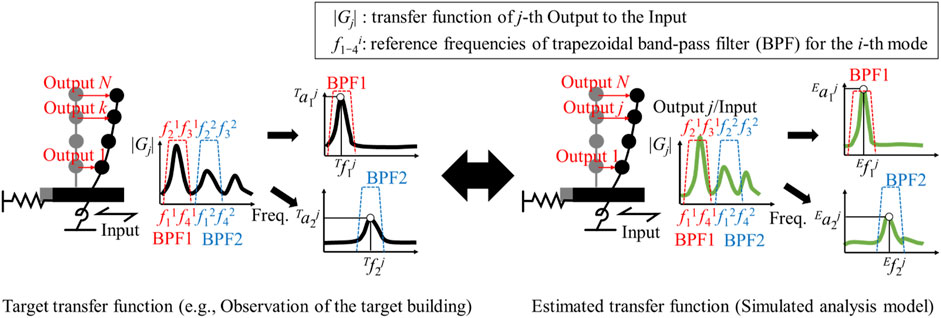
FIGURE 1. Conceptual diagram of the proposed framework.

2.2 MIEC method

This section presents an overview of the parameter identification flow using the MIEC method, according to the framework of a previous study (Uesaka et al., 2021b). For detailed steps of inverse analysis using MIEC, refer to previous research (e.g., Suzuki, 2018; 2019). The calculation in the MIEC method considers a nonlinear transform system F that outputs an N-dimensional vector {a₀} from an input M-dimensional parameter vector {p} based on Eq. 2:

$\begin{array}{c}\left\{a_0\right\}\\ N\times 1\end{array}=F\left(\begin{array}{c}\left\{p\right\}\\ M\times 1\end{array}\right),(2)$

where all vectors are treated as column vectors, F is assumed to be a frequency response analysis using a linear MDOF system SR model in our study. {p} comprises the shear stiffness and damping ratio of the superstructure and the spring stiffness, damping ratio, and damping coefficient of the dynamic soil spring (details are described later). {e₀} in Eq. 1a is used as the output vector {a₀} in this study. In other words, {p} is searched for such that the error vector is 0.

To correct an error in {a₀} iteratively, the perturbation impulse matrix $\left[B\right]$, comprising incremental output vectors when the perturbation {Δp} is added to the input, is recursively calculated. Subsequently, vector {Δα}, which satisfies Eq. 3, is calculated:

$\begin{array}{c}\left\{r\right\}\\ N\times 1\end{array}=\begin{array}{c}\left\{a_{\text{target}}\right\}\\ N\times 1\end{array}-\begin{array}{c}\left\{a_0\right\}\\ N\times 1\end{array}=\begin{array}{c}\left[B^{\prime }\right]\\ N\times M\end{array}\begin{array}{c}\left\{\Delta \alpha \right\}\\ M\times 1\end{array},(3)$

where $\left[B^{\prime }\right]$ is obtained by selecting the significant singular vectors in $\left[B\right]$ and the low-rank approximation of the matrix. $\left\{\Delta \alpha \right\}$ is the incremental ratio vector of the perturbation that corrects the residual error of output vector {r}, calculated using the low-rank approximated general-inverse matrix ${\left[B^{\prime }\right]}^{+}$, as shown Eq. 4:

$\begin{array}{c}\left\{\Delta \alpha \right\}\\ M\times 1\end{array}=\begin{array}{c}{\left[B^{\prime }\right]}^{+}\\ M\times N\end{array}\begin{array}{c}\left\{r\right\}\\ N\times 1\end{array},(4)$

Subsequently, {p} is iteratively modified using {Δα}, as shown Eq. 5, until the residual sum of squares (RSS) error (the norm of {r}) becomes smaller than an allowable tolerance:

$\begin{array}{c}\left\{p_{\text{new}}\right\}\\ M\times 1\end{array}=\begin{array}{c}\left\{p\right\}\\ M\times 1\end{array}+\begin{array}{c}\left\{∆p\right\}\\ M\times 1\end{array}\begin{array}{c}\circ \end{array}\begin{array}{c}\left\{∆\mathrm{\alpha }\right\}\\ M\times 1\end{array},(5)$

where “◦” represents the Hadamard product, {Δp}◦{Δα} is the correction vector of {p}, and {p_new} denotes the modified input vector.

2.3 Equation of motion and transfer function of the sway-rocking model

This section presents the target and estimated transfer function of the equations of motion of the SR model used in this study. The equation of motion of the SR model is expressed using Eqs 6–9. This equation is generally expressed as a relative displacement system with respect to the ground input motion displacement y, such as the free-soil surface response, as shown in Figure 2A, where k_i and c_i denote the shear stiffness and damping coefficients of the superstructure, respectively. K_H, C_H, K_R, C_R, K_HR(RH), and C_HR(RH) are the stiffness and damping coefficients of the sway,- rocking,-, and SR-coupled springs, respectively. m_i is the mass of each mass point, J₀ is the rotational inertial mass concentrated at the foundation, and H_i is the story height. Although the influence of SR-coupled springs has been proven to be non-negligible in pile foundations (Cristina et al., 2013), the effect is generally ignored. We show that parameter identification can be performed considering the effect of an SR-coupled spring. Note that the rotation angle of the seismic isolation layer and rocking angle of the foundation due to the rocking soil spring may be different, which is not shown in Figure 2. To simplify the following formulations, we adopted the equation of motion of the SR model, which ignores these differences in rotation angles. In the numerical experiments presented in Section 3, where the rotation angle of the seismic isolation layer and rocking angle of the foundation are different, we confirmed that the physical parameters can be identified according to the formulation in Section 2. The equation of motion for the SR model is as follows, where the time function is abbreviated as x(t) = x. In the numerical analysis in this research, the equation of motion was handled in the frequency domain; however, following equations are expressed in the time domain, because the actual observation records are time history data:

$\left[M\right]\left\{\ddot{x}\right\}+\left[C\right]\left\{\dot{x}\right\}+\left[K\right]\left\{x\right\}=-\left[M\right]\left\{e\right\}\ddot{y},(6)$

$\left[M\right]=diag\left[\begin{array}{cc}\begin{array}{cc}{m}_i& \cdots \end{array}& \begin{array}{ccc}{m}_1& m_0& J_0\end{array}\end{array}\right],(7)$

$\left[C\right]=\left[\begin{array}{cc}\begin{array}{cc}{c}_i& {-c}_i\\ {-c}_i& \ddots \end{array}& \begin{array}{lll}\cdots & & -c_i{H}_i\\ & & ⋮\end{array}\\ \begin{array}{cc}⋮& \\ & \\ -c_i{H}_i& \cdots \end{array}& \begin{array}{ccc}{c_1+c}_2& {-c}_1& c_2{H}_2{-c}_1{H}_1\\ {-c}_1& c_1+C_H& c_1{H}_1+C_{HR}\\ c_2{H}_2{-c}_1{H}_1& c_1{H}_1+C_{RH}& C_R+{\displaystyle \sum _{j=1}^n}{c}_j{H}_j^2\end{array}\end{array}\right],(8)$

$\left[K\right]=\left[\begin{array}{cc}\begin{array}{cc}{k}_i& {-k}_i\\ {-k}_i& \ddots \end{array}& \begin{array}{ccc}\cdots & & -k_i{H}_i\\ & & ⋮\end{array}\\ \begin{array}{cc}⋮& \\ & \\ -k_i{H}_i& \cdots \end{array}& \begin{array}{ccc}{k_1+k}_2& {-k}_1& k_2{H}_2{-k}_1{H}_1\\ {-k}_1& k_1+K_H& k_1{H}_1+K_{HR}\\ k_2{H}_2{-k}_1{H}_1& k_1{H}_1+K_{RH}& K_R+{\displaystyle \sum _{j=1}^n}{k}_j{H}_j^2\end{array}\end{array}\right],(9)$

where [M], [C], and [K] represent the mass, damping, and stiffness matrices, respectively. {$\left\{x\right\}={\left\{\begin{array}{cc}\begin{array}{cc}{x}_i& x_{i-1}\end{array}& \begin{array}{ccc}\cdots & x_0& {\theta }_0\end{array}\end{array}\right\}}^T$ is the relative displacement vector from the ground motion input point, and $\left\{e\right\}={\left\{\begin{array}{cc}\begin{array}{ccc}1& \cdots & 1\end{array}& 0\end{array}\right\}}^T$ is a state vector representing the inertial force distribution. In Eq. 6, the influence of foundation embedding is assumed to be relatively small, and the ground acceleration in the rocking direction is assumed to be zero.

FIGURE 2

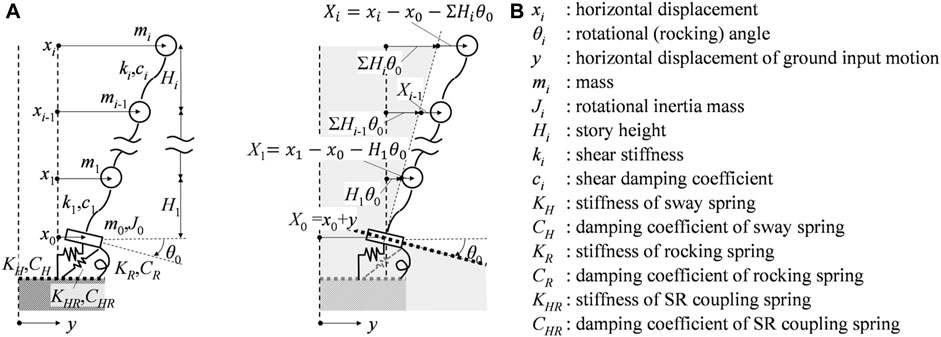
FIGURE 2. Concept of multi-degree-of-freedom system SR model. (A) Sway and rocking coupling system. (B) Sway separated from superstructure and rocking system.

In the previous studies, ground responses were often required to estimate building and soil spring parameters (e.g., Cristina et al., 2013). However, ground responses are not always observed. Therefore, in this study, the equations of motion were transformed to estimate these parameters without using the ground response. According to the method presented by Tojo and Nakai (2022) and Tojo et al. (2023), the equation of motion of the relative displacement system was considered with respect to the plane rotated by θ₀ from the horizontal plane shown in Figure 2B. Additionally, to reflect the influence of the SR coupling spring, we attempted to move the forces associated with the K_HR and C_HR terms on the right side, as shown in Eqs 10, 11; that is, they can be considered separately in the two equations. One includes the damping and stiffness matrices or coefficients [C_S], [K_S], C_R, and K_R for the superstructure and rocking soil spring. The other contains coefficients C_H and K_H of the horizontal soil spring. In addition, Eq. 11 becomes Eq. 12 when considering a vibration state ${\ddot{x}}_0\gg \ddot{y}$ in which the excitation force, such as the external wind force on the superstructure, is more dominant than the input ground motion:

$\left[\overline{M}\right]\left\{\ddot{X}\right\}+\left[\overline{C}\right]\left\{\dot{X}\right\}+\left[\overline{K}\right]\left\{X\right\}=-\left[\overline{M}\right]\left(\left\{e\right\}{\ddot{X}}_0+\left\{H\right\}{\ddot{\theta }}_0\right)+{\overline{f}}_{x_0},(10)$

$m_0{\ddot{X}}_0+C_H{\dot{x}}_0+K_H{x}_0=c_1{\dot{X}}_1+k_1{X}_1+{\overline{f}}_{{\theta }_0},(11)$

$m_0{\ddot{x}}_0+C_H{\dot{x}}_0+K_H{x}_0=c_1{\dot{X}}_1+k_1{X}_1+{\overline{f}}_{{\theta }_0},(12)$

$\left[\overline{M}\right]=\left[\begin{array}{cc}\left[M_S\right]& \\ \left[M_{BS}\right]& J_0\end{array}\right],(\mathrm{13a})$

$\left[M_S\right]=diag\left[\begin{array}{ccc}{m}_i& \cdots & m_1\end{array}\right],(\mathrm{13b})$

$\left[M_{BS}\right]=\left[\begin{array}{ccc}{m}_i\sum H_i& \cdots & {m_{1}H}_1\end{array}\right],(\mathrm{13c})$

$\left[\overline{C}\right]=\left[\begin{array}{cc}\left[C_S\right]& \\ & C_R\end{array}\right],\left[C_S\right]=\left[\begin{array}{cc}\begin{array}{cc}{c}_i& {-c}_i\\ {-c}_i& \ddots \end{array}& \\ & {c_1+c}_2\end{array}\right],(14)$

$\left[\overline{K}\right]=\left[\begin{array}{cc}\left[K_S\right]& \\ & K_R\end{array}\right],\left[K_S\right]=\left[\begin{array}{cc}\begin{array}{cc}{k}_i& {-k}_i\\ {-k}_i& \ddots \end{array}& \\ & {k_1+k}_2\end{array}\right],(15)$

${\overline{f}}_{x_0}=-\left\{\begin{array}{c}0\\ C_{HR}\end{array}\right\}{\dot{x}}_0-\left\{\begin{array}{c}0\\ K_{HR}\end{array}\right\}{x}_0,(\mathrm{16a})$

${\overline{f}}_{{\theta }_0}=-C_{HR}{\dot{\theta }}_0-K_{HR}{\theta }_0,(\mathrm{16b})$

where $\left[\overline{M}\right]$, $\left[\overline{C}\right]$, and $\left[\overline{K}\right]$ are the matrices of Eqs 13a–13c, Eq. 14, and Eq. 15, $\left\{X\right\}={\left\{\begin{array}{cc}\begin{array}{cc}{X}_i& X_{i-1}\end{array}& \begin{array}{ccc}\cdots & X_1& {\theta }_0\end{array}\end{array}\right\}}^T$ is the relative displacement vector corresponding to the building shear deformation excluding the rocking displacement from the foundation mass point, and $\left\{H\right\}={\left\{\begin{array}{cc}\begin{array}{cc}\sum H_i& \sum H_{i-1}\end{array}& \begin{array}{cc}\cdots & H_1\end{array}\end{array}\right\}}^T$ is the height vector.

Subsequently, considering the transfer function of the response to the input when the external forces ${\overline{f}}_{x_0}$ and ${\overline{f}}_{{\theta }_0}$ defined by Eqs 16a, b on the right sides of Eqs 10, 12 are ignored, Eqs 17a, 17b, and Eq. 18 are obtained, respectively. In this study, Eqs 17a, 17b were used as the target or estimated transfer function to identify the physical parameters related to the superstructure and rocking soil spring. Eq. 18 was utilized to identify the parameters of the horizontal soil spring. The effect of the SR coupling spring could be considered because ${\overline{f}}_{x_0}$ and ${\overline{f}}_{{\theta }_0}$ were treated as arbitrary external forces that satisfied the target transfer function of Eqs 17a, 17b, and Eq. 18:

$G_{k\text{FL}}=\frac{{\ddot{X}}_k+{\ddot{X}}_0+\sum H_k{\ddot{\theta }}_0}{{\ddot{X}}_0+\sum H_k{\ddot{\theta }}_0}=\frac{{\ddot{U}}_k}{{\ddot{X}}_0+\sum H_k{\ddot{\theta }}_0},(\mathrm{17a})$

$G_R=\frac{{\ddot{\theta }}_0}{{\ddot{X}}_0+H_{eq,R}{\ddot{\theta }}_0},(\mathrm{17b})$

$G_H=\frac{{\ddot{x}}_0}{X_1},(18)$

$H_{eq,R}=\frac{H_1^2+\dots +{\left(\sum H_i\right)}^2}{H_1+\dots +\sum H_i},(19)$

where G_kFL and G_R represent the transfer functions when the horizontal absolute acceleration response of kth floor of the superstructure or the rocking absolute acceleration response of the foundation mass point is divided by the horizontal effective acceleration input. The horizontal effective acceleration input is defined as the input obtained by multiplying the foundation rocking input times the height of each floor and adding it to the ground motion. G_H is the transfer function of the horizontal absolute acceleration response of the foundation mass point to the horizontal relative displacement response of first floor to the foundation mass point. ΣH_k is the height up to kth floor, and H_eq,R defined by Eq. 19 is the equivalent height of the rigid-body rocking mode proposed by Tojo and Nakai (2022). By considering the transfer functions of two separate equations in this way, the superstructure and dynamic soil spring can be estimated without using the ground response. However, Eqs 17a, 17b must handle the response when an earthquake is input, and Eq. 18 must handle the response when an external force is applied to the superstructure.

3 Verification of the proposed method using numerical analysis

This section describes the application of the system identification method using the proposed framework detailed in the previous section to the response results obtained through the seismic response analysis using the SR model, whose vibration characteristics are known. Subsequently, an assessment was performed to confirm whether each physical parameter set for the numerical analysis was accurately evaluated. The purpose of the numerical simulation was to confirm whether the stiffness and damping of the superstructure and dynamic soil springs could be appropriately evaluated using the proposed framework. In actual buildings, obtaining seismic observation data that involve foundation damage is difficult. Furthermore, the damping characteristics of the ground vary widely. Therefore, to confirm these effects, we changed the stiffness and damping parameters of the dynamic soil spring.

3.1 Analysis overview

The analysis object was an SR model of a five-mass system with mass i = 5 in Figure 2. Tables 1, 2 list the specifications of the superstructure and soil springs of the SR model. Numerical analyses were performed in the frequency domain so that the analytical model for the superstructure and SR soil springs was linear. The specifications were set as a model of the short-side direction based on the stiffness and mass in the seismic design of an existing reinforce concrete (RC) BI building with three stories. Section 4 describes the building details. Because the study subject was a shear-type building with a seismic-resistant wall above the BI layer, it was modeled as an equivalent shear-type beam element with a sufficiently large bending stiffness. The rotational inertial masses of the floors above the BI layer were consolidated into first floor (referred to 1FL in Table 1). The damping constant was the average value based on the measured database of RC buildings (Architectural Institute of Japan, 2020). The BI layer was modeled as a bending shear beam, considering the shear and bending stiffnesses and damping constant based on the design values. The damping of the superstructure is treated as the complex stiffness k_i^* = k_i (1 + i2h_i). The foundation comprised cast-in-place concrete piles. Tables 3, 4 list the foundation and soil specifications, respectively. The damping constants of each soil layer were set based on the relationship between the Q-value and the S-wave velocity (V_S) (Architectural Institute of Japan, 1987). Each soil spring of Table 2 was calculated by using the thin-layer element method (TLM) (e.g., Tajimi and Shimomura, 1976) based on the specifications in Tables 3, 4. Furthermore, the spring stiffness and damping of the soil springs were approximated as constants according to the method of the Architectural Institute of Japan (2006). In addition, in Table 2, the values of the SR springs assuming that the piles were damaged are listed in each lower row. These SR springs considering damaged pile were calculated by setting the cross-sectional area of more than half of the pile heads with length 0.25 m to 1/10. The arrangement of the piles is the same position as the seismic isolation device shown in section 4.

TABLE 1

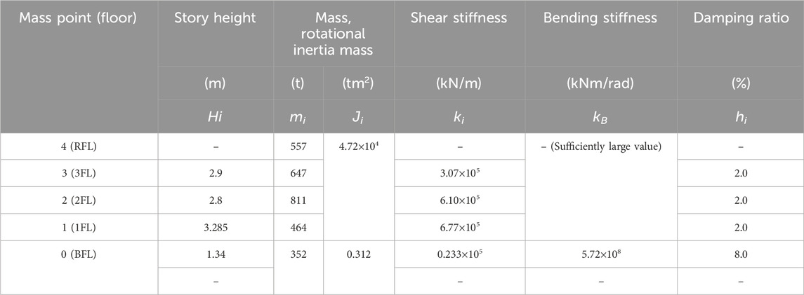
TABLE 1. Specifications of analysis model. Properties of superstructure of SR model. Each symbol follows the description in Figure 2.

TABLE 2

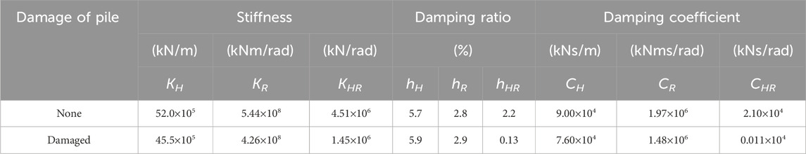
TABLE 2. Specifications of analysis model. Properties of soil springs. Each symbol follows the description in Figure 2.

TABLE 3

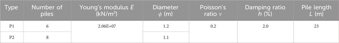
TABLE 3. Specifications of analysis model. Properties of pile.

TABLE 4

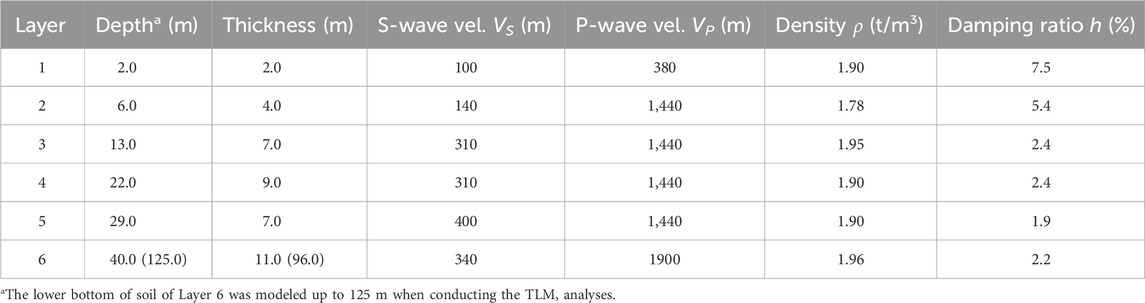
TABLE 4. Specifications of analysis model. Properties of soil.

Figures 3A, B show the acceleration time–history waveforms and acceleration response spectra of the input seismic motions. Three earthquake motions were used as input seismic motions: the first was a white noise wave with little bias due to its spectral characteristics (hereinafter referred to as WN); the second was an east to west direction component of the KiK-net Haga observation wave published by National Research Institute for Earth Science and Disaster Resilience, 2019 obtained from the 2011 Tohoku Earthquake (hereinafter referred to as Haga); and the third was artificial designed seismic motion provided by the Building Center of Japan, 1992 (hereinafter referred to as Dgn). The duration and sampling time were 81.92 and 0.01 s, respectively. In the numerical analysis, scenarios receiving the seismic input or external force of wind were assumed and the following cases were considered. Note that, in the discussion presented in Section 3.4, the transfer functions of Eqs 17a, 17b were evaluated in Analysis (1), and that of Eq. 18 in Analysis (2). Specifically, Analysis (1) was a seismic response analysis, where each seismic motion was input through the soil spring in the horizontal direction, and Analysis (2) was a excitation analysis of the superstructure, where the acceleration excitation of the WN was input in the horizontal direction to the mass point of 1FL of the superstructure.

FIGURE 3

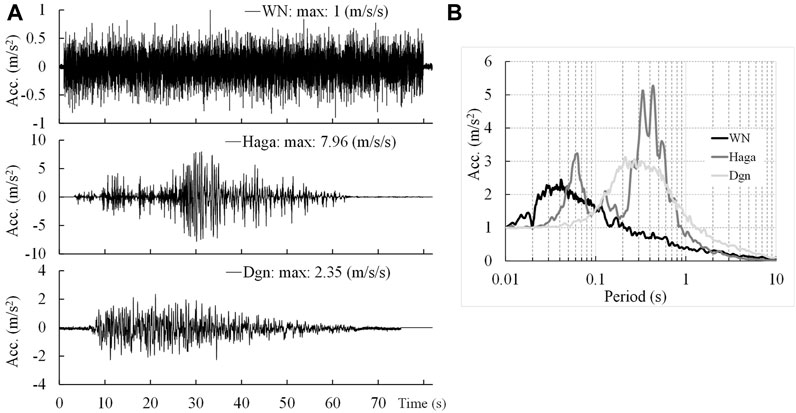
FIGURE 3. Input excitation motion for analysis. (A) Acceleration time history (from bottom to top: Dgn excitation, Haga excitation, WN excitation). (B) Acceleration response spectrum with the maximum value in the acceleration time history normalized to 1.0 (h = 5%).

3.2 Numerical analysis case

Recent studies (e.g., Architectural Institute of Japan, 2020; Cruz and Miranda, 2021) have shown different trends in the damping properties of architectural structures. In one trend, the attenuation of higher-order modes increased with increasing frequency. Another trend maintained approximately constant attenuation of the lower and higher modes. Considering these findings, to examine the applicability of the proposed framework to indirect monitoring of soil and foundations, we conducted an analysis in which the stiffness was varied assuming damage to the piles. Furthermore, we confirmed the effects of differences in the damping characteristics of the ground on the identification results.

Table 5 lists the numerical analysis cases. Four cases were evaluated in this study, denoted by the initials “N” and “D” for cases with undamaged and damaged piles, respectively, as listed in Table 2. In addition, “-C” denotes the case in which the damping constants (h_H, h_R, h_HR) of the dynamic soil spring in the horizontal and rocking directions were used to provide a constant divergent damping to the vibration frequency. “-P” indicates the case in which the damping was proportional to the vibration frequency using each damping coefficient (C_H, C_R, C_HR). Table 5 shows the natural frequencies and damping constants obtained through the complex eigenvalue analysis (e.g., Terazawa and Takeuchi, 2018) based on the complex stiffness of the SR model in each case, along with the results of the foundation-fixing condition (FB). Focusing on the differences between the damping models, although the natural frequencies of N-C and N-P or D-C and D-P were nearly the same, differences in the damping characteristics of the primary and secondary modes were observed.

TABLE 5

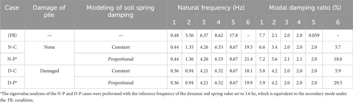
TABLE 5. Analysis cases and properties of identified parameters. Analysis cases and vibration characteristics.

3.3 Analysis condition of the MIEC method

The input parameters identified, denoted as {p} in Eq. 2, were the stiffness and damping constants or damping coefficients (k_i, K_H, K_R, K_HR, h_i, h_H, h_R, and h_HR or C_H, C_R, and C_HR) of each part shown in Table 1. We assumed that the bending stiffness k_B of the BI layer was known. In the MIEC method, the initial values and perturbation quantities of each parameter to be identified should be provided; Table 6 lists the initial values and perturbation quantities of each parameter. The initial values provided in the inverse analysis were rounded to a power of 10, assuming that the approximate value of each parameter could be estimated in advance. For convenience, the amount of perturbation of the shear stiffness was defined relative to the shear stiffness k_i multiplied times the story height H_i. {p_new}, obtained from Eq. 5, was set as the difference from the initial value. This difference was added to the initial values and input into the analytical model. Because each parameter (K_HR, h_HR, and C_HR) related to the SR-coupled spring was an external force satisfying the relation in Eqs 17a, 17b, and Eq. 18, negative values were allowed. The other parameters were treated as absolute values. The perturbation {Δp} for each parameter was approximately 1/10 to 1 times the initial value of each parameter. Assuming an observation error for each response acceleration time history obtained in the analysis, the target transfer function was calculated by adding noise with a signal-to-noise (SN) ratio of 100. The noise was generated based on a normal distribution with a mean of 0 and standard deviation of 0.1. The SN ratio was defined as the ratio of the variance of each response in the numerical analysis to the variance of the noise. The number of modes to be selected for matrix $\left[B^{\prime }\right]$ in Eq. 3 was determined using the norm ratio of the error vector in the study by Suzuki (2019), and the threshold of the norm ratio was 0.3. The convergence threshold of the RSS error was 0.03, and the maximum number of repetitions was 150. However, if a tendency for convergence to a smaller error was observed, the maximum number of repetitions was increased to 300. The maximum dominant response extracted by the band-pass filter was set to be up to the fifth-order mode, which could be determined visually. The response of the observation point used for identification was assumed to be BFL, 1FL, and RFL only, considering the installation position of the sensor in the actual building, as shown in Section 4. The target transfer function was calculated according to Eqs 17a, 17b, and Eq. 18 using the respective horizontal and rotational acceleration responses or the displacement response obtained from those responses. Figures 4A–C respectively show the target transfer function and trapezoidal filter for the N-P, N-C, and D-P cases as examples of a band-pass filter setup for extracting the dominant response. The estimated transfer functions are also shown in these figures, as are the transfer functions for the unmeasured floors. Each physical parameter was identified using the following procedure.

TABLE 6

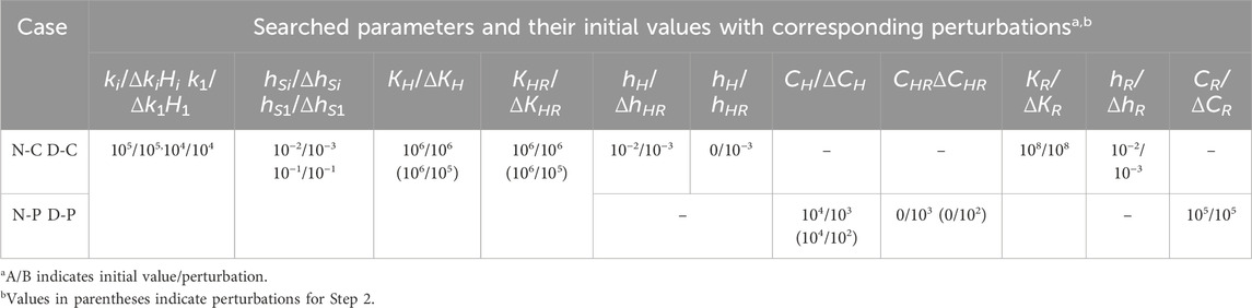
TABLE 6. Analysis cases and properties of identified parameters. Initial values and perturbations of each analysis case.

FIGURE 4

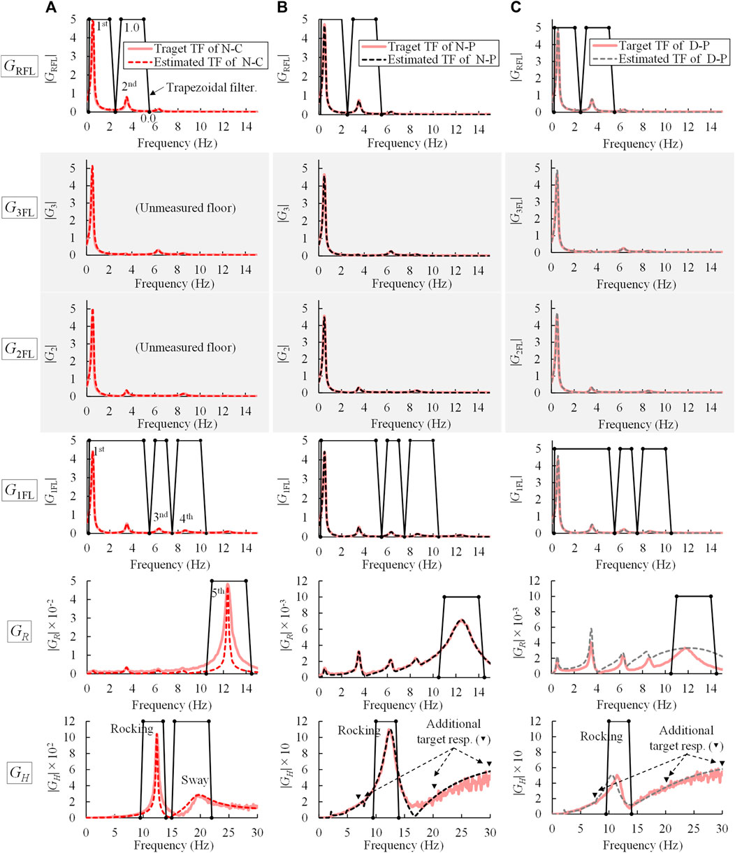
FIGURE 4. Target and estimated transfer functions (TFs) and trapezoidal band-pass filter for extraction in each mode for representative cases (from top to bottom: $G_{\text{RFL}}={\ddot{U}}_4/\left({\ddot{X}}_0+{\sum }_{i=1}^4{H}_i{\ddot{\theta }}_0\right)$, $G_{3\text{FL}}={\ddot{U}}_3/\left({\ddot{X}}_0+{\sum }_{i=1}^3{H}_i{\ddot{\theta }}_0\right)$, $G_{2\text{FL}}={\ddot{U}}_2/\left({\ddot{X}}_0+{\sum }_{i=1}^2{H}_i\right)$, $G_{1\text{FL}}={\ddot{U}}_1/\left({\ddot{X}}_0+H_1{\ddot{\theta }}_0\right)$, $G_R={\ddot{\theta }}_0/\left({\ddot{X}}_0+H_{eq,R}{\ddot{\theta }}_0\right)$, and $G_H={\ddot{x}}_0/X_1$.) (A) N-C. (B) N-P. (C) D-P.

Step 1. All physical parameters were temporarily identified based on the transfer function of Eqs 17a, 17b. (The target and estimated values are shown in Figures 4A–C as G_RFL, G_1FL, and G_R, respectively). In this step, repeated calculations were performed based on the initial values and amount of perturbation in Table 6. The dominant responses from six points were extracted: the first- and second-order peaks for G_RFL; the first-, third-, and fourth-order peaks for G_1FL; and the fifth-order peak for G_R in Figures 4A–C, respectively. Basically, the number of points for extracting the dominant response of the transfer function could be the same as the maximum objective mode order. However, in the first mode of a BI building, the superstructure was considered to move as an almost rigid body. To incorporate this constraint, we selected the dominant mode for both 1FL and RFL when extracting the first-order mode (e.g., see the notation “first” in Figure 4A).

Step 2. K_H, K_HR, h_H h_HR, and h_R or C_HR, C_HR, and C_R were identified again based on Eq. 18. The transfer functions based on Eq. 18 are shown in Figures 4A–C as G_H. The initial values and perturbations of the parameters to be identified in Step 2 were used from the values in Table 6. The initial values of the other parameters were fixed using the values obtained in Step 1. The dominant modes selected were up to two peaks. One was the mode in which the horizontal response of foundation was predominant (represented as Sway in Figure 4A). The other was excited by the rocking response due to the effect of the SR coupling spring (represented as Rocking in Figures 4A–C). However, for N-P and D-P, which had large dissipative damping at high frequencies, the high-frequency peak at approximately 20 Hz present in the N-C case was not observed and amplitude increased monotonically. Therefore, by adding amplitudes at 7.5, 20, and 30 Hz as fitting point of the target transfer function, we attempted to improve the parameter identification accuracy by capturing the shape of the transfer functions (see the symbols ▾ in Figures 4A–C).

3.4 Identification results for the numerical test

3.4.1 Confirmation of validity and identification accuracy of the proposed method

The validity of the formulation and identification accuracy of the proposed method are discussed with respect to the results of the numerical experiments. First, to verify the proposed method, we will discuss the seismic response analysis using WN excitation waves so that higher-order modes can be sufficiently considered. The results shown below are the identification values at the minimum error when the number of iterations was sufficiently large, and the allowable value of the RSS error or maximum number of iterations was reached in all cases in Steps 1 and 2.

Figures 5A, B show the identification results for the shear stiffness and damping constants of the superstructure. The initial value (Init.) and correct answers are presented in the same figure. Figures 5A, B depict the 10% and 20% error ranges, respectively. Figure 5A reveals that the stiffness of the superstructure is accurately identified in each case, and the maximum identification error is approximately 10%, including the BI layer (BFL). Considering the damping in Figure 5B, the error is slightly larger than the stiffness in each case, and the error is approximately 20% in N-C and D-C. However, the error is larger in N-P and N-C, where the dissipative damping is proportional to the frequency, and the variation in each layer tends to increase. This trend occurs is because damping is generally susceptible to noise, and the estimation accuracy of damping tends to deteriorate compared with that of the stiffness. Additionally, the dissipative damping of dynamic soil springs increases proportionally to the vibration frequency, which can make evaluation of the damping characteristics of the superstructure even more difficult.

FIGURE 5

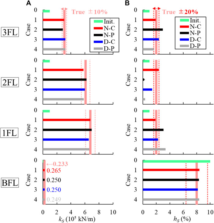
FIGURE 5. Identification results of superstructure (from bottom to top: BFL, 1FL, 2FL, and 3FL). (A) Shear stiffness. (B) Damping ratio.

Table 7 lists the identification results for the spring stiffness of the dynamic soil spring in each case, and Table 8 presents the identification results for the damping constant or damping coefficient. In each table, the identification results of Steps 1 and 2 and the error ratio of the identification result to the true value are shown, with the largest error among the four cases shaded in red. Table 7 reveals that the rocking spring stiffness shows good identification accuracy, except for D-P. The sway spring stiffness exhibits good accuracy, similar to the rocking spring stiffness for N-C and D-C in Step 2; however, the error reaches approximately 35%–60% for N-P and D-P. In step 1, the degree of freedom of the foundation mass point is excluded, as shown in Eqs 17a, 17b. Thus, determining the parameters of the horizontal dynamic soil spring in this step is inappropriate.

TABLE 7

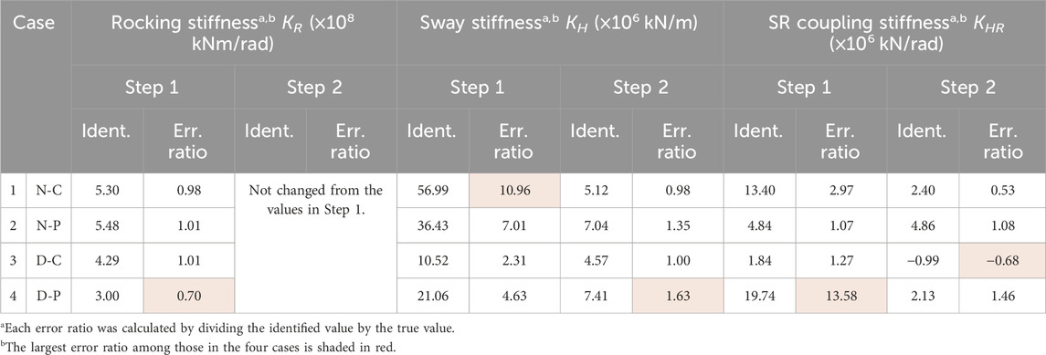
TABLE 7. Identification results of soil spring stiffness. Soil spring stiffness.

TABLE 8

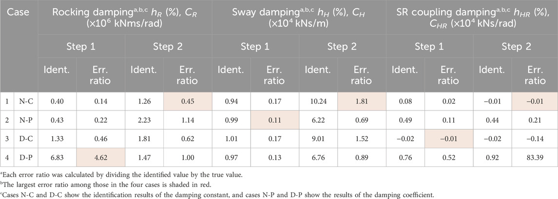
TABLE 8. Identification results of soil spring stiffness. Soil spring damping.

Table 8 shows that the damping accuracies of the rocking and sway springs are improved in Step 2 compared with those in Step 1. However, the maximum error is approximately 55%–80%. The accuracy of the damping constant estimation is lower than that of the stiffness in Table 7.

The above results confirm the appropriateness of the proposed framework considering higher-order modes. As the high estimation accuracies of the stiffnesses of both the superstructure and soil spring in each step were subjected to the WN excitations, the proposed method is applicable to the SHM of the superstructure and the indirect monitoring of the soil and foundation. However, one limitation of this method is that the estimation accuracy of damping is slightly lower than that of the stiffness of each part, indicating the potential for improvement. Note that the stiffness and damping of the SR-coupled spring shown in Tables 7, 8 differ from the true values in Steps 1 and 2. They are treated as arbitrary external forces adjusted to minimize the error with respect to the transfer function in Eqs 17a, 17b, and Eq. 18; therefore, their accuracies should not be evaluated.

3.4.2 Effects of pile damage and differences in the damping model of soil

This section discusses the effects of the pile damage degree and different damping models of dynamic soil springs on the identification accuracy of the physical parameters of the superstructure and soil springs. Furthermore, based on the identification results of the physical parameters when seismic motions with different spectral characteristics were input, we will discuss the influence of the presence or absence of excitation of higher-order modes on the identification results of vibration characteristics.

Figure 6A compares the coherence for the input and output of the target transfer functions of G_RFL, G_1FL, and G_R for the N-C, N-P, D-C, and D-P cases with WN excitation. To obtain each coherence, a 512-sample Hamming window was used. The overlap between adjacent segments was specified as 500 samples, and the number of discrete Fourier transform points was 2000. In Figure 6, the frequencies of the first-to fifth-order modes extracted at the transfer function shown in Figure 4 are indicated by ▾ markers. Figure 6A demonstrates that with WN excitation, a noticeable difference exists in the fifth mode. The frequencies at which the coherence decreases due to pile damage differ between N-C and D-C. In contrast, no significant difference in coherence exists near the fifth-order mode between N-P and D-P, which have large dissipative attenuation. This finding suggests that the dominant response is difficult to capture. Furthermore, the comparison of the estimated and target transfer function of G_R in Figures 4B, C shows that the estimation accuracy of the transfer function for N-P without pile damage is better. Therefore, the decrease in the stiffness estimation accuracy for D-C in Table 7 is thought to occur because the dominant response is the lowest due to both the decrease in soil spring stiffness owing to pile damage and the large dissipative damping. This result suggests that not only the dominant response of the transfer function, but also the shape of the envelope of the transfer function need to be reproduced. In addition, when the dissipative damping is large, as shown in Figures 4B, C, the dominant response at high frequencies of G_H disappears. In such cases, even if the transfer function is fitted at multiple points to reproduce envelope of the transfer function, the stiffness estimation accuracy may be limited.

FIGURE 6

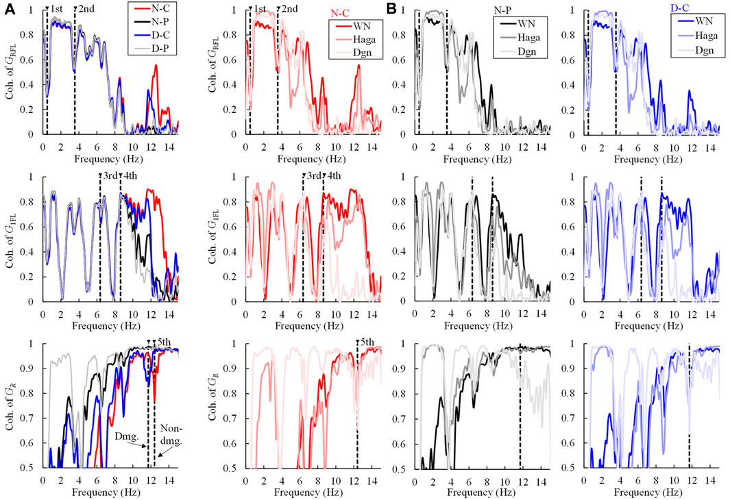
FIGURE 6. Comparison of coherence for input and output of target transfer functions (from bottom to top: G_R, G_1FL, and G_RFL). (A) Comparison of N-C, N-P, D-C, and D-P cases with WN excitation. (B) Comparison of N-C, D-C, and D-P cases with WN, Haga, and Dgn excitation.

Next, we will describe the identification results of each parameter when the spectral characteristics of the input seismic motion are different. Figure 6B compares the coherence of N-C, N-P, and D-P when each of the three earthquake motions shown in Figure 3 is input. From bottom to top, the order is G_RFL, G_1FL, and G_R. In Figures 6A–C, the differences in G_RFL due to each earthquake motion are small. However, the values near the fourth- and fifth-order modes of G_1FL and G_R are significantly reduced in the case of Dgn, which does not contain many high-frequency components. Table 9 compares the identification results of each physical parameter when the input seismic motion is changed for the N-C, N-P, and D-C cases. The table shows the error ratio of the identification results relative to the correct values. Items with error ratios exceeding 20% are shaded in red. The RSS error of the transfer function is also listed in parentheses in each case. Basically, the larger the RSS error, the larger the error ratio of the identification result relative to the true value. All BFL results corresponding to seismic isolation layers show generally good estimations. However, in the case of the Dgn excitation with almost no frequency components in higher-order modes, the estimation accuracy of not only the superstructure, but also the soil springs decreases significantly, especially in N-P and D-C, corresponding to the large decrease in the coherence of the higher-order modes (see Figure 6B). In the Haga excitation case, the identification results are more accurate than those in the Dgn case. This finding suggests that actual earthquake motion excites a certain amount of high-frequency components; therefore, the number of samples of earthquake motion must be increased to improve the estimation accuracy of physical parameters.

TABLE 9

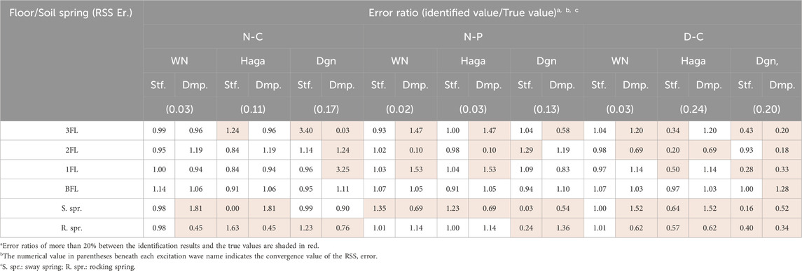
TABLE 9. Identification results of soil spring stiffness. Error ratios of stiffness and damping of superstructures and soil springs when changing the input ground motion.

The above results confirm that when the decrease in stiffness due to foundation damage or the dissipative damping of the ground or both are large, the identification accuracy of physical parameters tends to decrease. Furthermore, if higher-order modes are not excited due to the spectral characteristics of seismic motion, the accuracy of parameter identification also tends to decrease. Thus, considering higher-order modes for the identification of physical parameters in BI buildings is important. Most conventional identification methods for BI buildings use single-mass point systems for the superstructure and evaluate the behavior of the seismic isolation layer (e.g., Furukawa et al., 2005). However, in recent years, the importance of considering second- and higher-order modes when evaluating the superstructure above the seismic isolation layer has been highlighted (Astroza et al., 2021; Hernandez et al., 2021; Yu et al., 2023). In addition, our research results show that considering higher-order modes is important when estimating the health of not only the superstructure, but also the dynamic soil springs.

Note that the above results indicate that the estimation accuracy of the physical parameters of the soil springs may decrease because the proposed method uses only the dominant response of one point. The reproducibility of the shape of the transfer function parabola could be important for the estimation both of stiffness and damping characteristics. This aspect is a subject for future investigation.

4 Application to an actual BI building

As described in this section, the aging and amplitude dependence of superstructures and dynamic soil springs were analyzed by applying the proposed method to a seismically isolated building of a three-story RC structure on the ground and identifying the physical parameters considering higher-order modes. Long-term seismic observations, including the 2011 Tohoku Earthquake, have been conducted in this building. Additionally, the aging of seismic isolators was investigated previously (Higashino et al., 1997; Hamaguchi and Yamamoto, 2005; Kyuuke et al., 2005; Hamaguchi et al., 2009; Hamaguchi and Sasaki, 2009; Yamamoto, 2011; Kamoshita et al., 2018; Tanaka et al., 2018). For details on this building or seismic isolators, please refer to the aforementioned literature. However, analysis of the physical parameters of the superstructure, soil, and foundation has not been conducted. In general, the amplitude dependence of the damping and stiffness of buildings is well known (e.g., Architectural Institute of Japan, 2020), but for BI buildings, the seismic isolation system adopted differs depending on the building, and some unclear points remain. Therefore, analyzed data must be accumulated.

4.1 Overview of the building and seismic observation records

Figures 7A, B show plan views of BFL, 1FL, and RFL and the elevation in the direction of the short side of the building, respectively. The locations of the accelerometers installed on each floor are indicated in the plans. Measurements were not taken for 2FL or 3FL. This building is a three-story RC BI building completed in 1987. The foundation is a pile foundation comprising cast-in-place concrete piles. The BI layer comprises 14 natural-rubber-based laminated rubbers and eight viscous dampers. The arrangement of the piles is the same position as the laminated rubbers. Approximately 10, 22, and 30 years after the completion of construction, one laminated rubber piece was removed, and an aging investigation was conducted (Higashino et al., 1997; Hamaguchi et al., 2009; Kamoshita et al., 2018). According to Kamoshita et al. (2018), the vertical stiffness of laminated rubber increased with aging, with a fluctuation range of approximately 19%–2%. Regarding the horizontal stiffness of the same member, the effect depended on the evaluation section of shear strain γ. It tended to decrease from the time of shipment in the γ = 10%–50% section, but increased from the time of shipment in the γ = 10%–200% section. The former decreased by −16%–7%, and the latter increased by 7%–14%. The aging of viscous dampers for approximately 20–30 years has also been investigated (Hamaguchi and Sasaki, 2009; Tanaka et al., 2018). The shear resistance obtained by sampling a part of the viscous body was estimated to be approximately −2%–4% of the standard value. These investigation results confirmed that no remarkable aging occurred, although minor variations were observed. Figure 7C shows the number of seismic waves, maximum absolute acceleration, inter-story velocity, and inter-story deformation angle recorded annually from June 2007 to March 2023 in BFL when the physical parameters were evaluated. For the inter-story velocity and inter-story deformation angle, the relative velocity and relative displacement were obtained by integrating the absolute acceleration in BFL and 1FL once or twice, respectively, and the inter-story deformation angle was calculated by dividing the relative displacement by the story height of the BFL. The magnitude of the responses increases significantly in 2011, as recorded during the 2011 Tohoku Earthquake. Excluding these responses, the maximum responses recorded from 2007 to 2023 vary slightly; however, most are small earthquakes with maximum accelerations of less than 100 cm/s². The maximum inter-story deformation angle is less than 1% rad excluding that in 2011, and the deformation of the BI layer is extremely small.

FIGURE 7

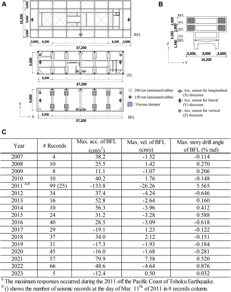
FIGURE 7. Floor plan with installation position of the accelerometer, directional elevation plan of evaluated base-isolated building, and overview of earthquake observation records. (A) Floor plans of BFL, 1FL, and RFL. (B) Lateral directional elevation plan. (C) List of observation records.

4.2 Analysis condition of MIEC method

The physical parameters for the observation records were identified based on the five-mass point system SR model used in Section 3. The observational records evaluated were on the short side of the building. The identified physical parameters were the same as those in Section 3. Table 6 was also referenced for the amount of perturbation of each physical parameter. The initial values of the parameters based on the design values in Tables 1, 2 were used. However, each initial value of the SR-coupled spring was set to zero in accordance with normal seismic design. As obtaining the damping characteristics of soil springs in advance is difficult, the damping model of the dynamic soil spring was examined in advance using two types of models: one with constant dissipative damping (damping constant) with respect to frequency (case C in Section 3) and another with damping proportional to the frequency (case P). As a result, the model with case C was used owing to its low RSS error. These analysis conditions were common for all earthquake motions.

Wind observations were not conducted at the target buildings, and only strong motion observation records were obtained. Therefore, only Eqs 17a, 17b were considered in this analysis. The target transfer functions were G_R, G_1FL, and G_RFL from the responses of BFL, 1FL, and RFL, where the accelerometers were installed. Among the physical parameters, the identification values of h_R, K_H, and h_H in addition to the stiffnesses K_HR and h_HR of the SR-coupled spring were not analyzed in detail. Regarding the acceleration response used for the input and output, the horizontal direction was the average value of the horizontal accelerometers at both ends in the X-direction, as shown in Figure 7A. The rocking direction responses were calculated from the difference in the vertical accelerometers at both ends in the Y-direction in the BFL divided by the distance. The number of dominant response modes extracted was of the fifth order. The band-pass filter settings for extracting the dominant response were set by obtaining the average value of the transfer function based on the seismic observation records and visually judging the dominant modes. Figures 8A, B show the target transfer function based on the observation record and the estimated transfer function based on the identification results, respectively. The estimated transfer function was calculated using the regression equation of the physical parameters and the relationship between the average amplitude, which will be described later. The extraction target was from the first to fifth mode. The primary mode shown in Figure 8A was applied to G_1FL and G_RFL to consider the constraint of the rigid-body mode, as described in Section 3. The fourth and fifth modes had large response variations and were unclear. Therefore, the extraction range of the filter was relatively large. Determining the extraction method for the dominant response in such cases requires further investigation. Comparing the transfer functions in Figures 8A, B, the dominant responses of the target and estimated transfer functions generally correspond well for the first-to third-order modes (see approximately 1, 7, and 11 Hz in the figures). There is room for improvement in the consistency of higher-order modes beyond the fourth order and the accuracy of the rocking response of G_R.

FIGURE 8

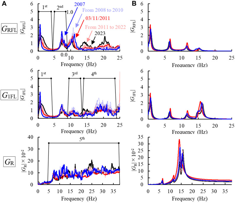
FIGURE 8. Target transfer functions with trapezoidal filter of each mode and estimated transfer functions (from bottom to top: G_R, G_1FL and G_RFL). (A) Observation results. (B) Analysis results.

4.3 Discussion on aging and amplitude dependence of each parameter

This section presents an analysis of the aging and amplitude dependence of the physical parameters identified based on the analysis conditions described in the preceding paragraph.

Figure 9A shows the average value μ, maximum value (Max.), and minimum value (Min.) for all annual seismic waves of the maximum inter-story deformation angle of the foundation floor (BFL). However, for 2011, the results for March 11, including the 2011 Tohoku Earthquake, and the succeeding results were calculated separately. The 2010 and 2012 periods, before and after 2011, are hatched in yellow and shown separately. The results in Figures 9B–G are also hatched in the same way. The average maximum inter-story deformation angle shown in Figure 9A is approximately 0.1% rad or less in each year, except on 11 March 2011. No significant differences are observed; however, after 2015, earthquakes with relatively small responses dominate.

FIGURE 9

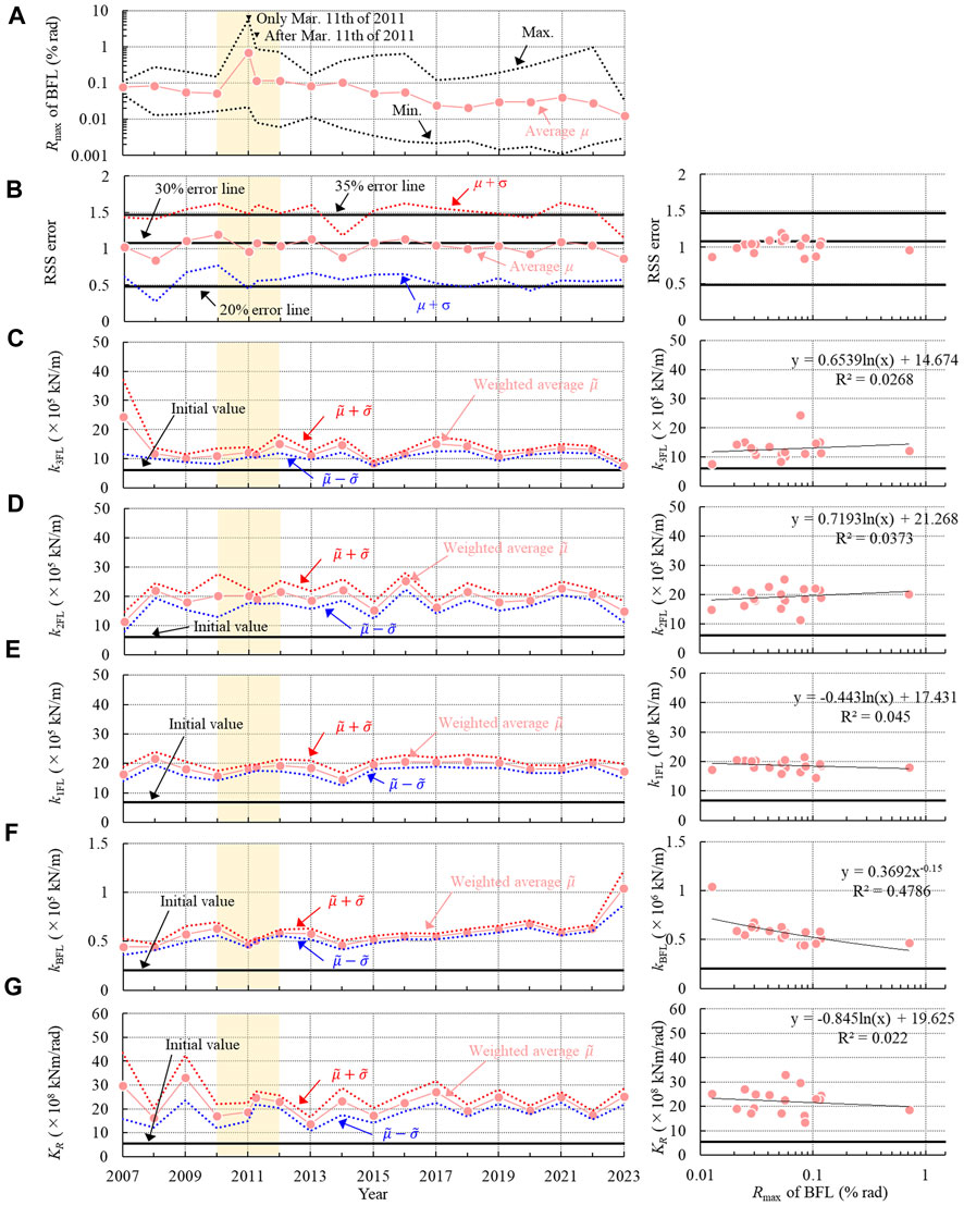
FIGURE 9. Aging and amplitude dependence of stiffness for superstructure and soil spring. (A) Average of maximum drift angle of BFL. (B) RSS error. (C) Stiffness of 3FL. (D) Stiffness of 2FL. (E) Stiffness of 1FL. (F) Stiffness of BFL. (G) Stiffness of rocking spring.

The left side of Figure 9B shows the RSS error of the target and estimated transfer function in each year. The legend shows the mean μ and standard deviation ±σ within a single year. The right side of Figure 9B shows the relationship between the average maximum inter-story deformation angle R_max shown in Figure 9A and the average RSS error. The solid black lines in Figure 9B represent the lines when the errors are 20%, 30%, and 35%. The average error is approximately 30% in each year. The bias of the identification result depending on the spectral characteristics of the ground motions was smoothed to a certain degree through averaging. Observing the amplitude dependence diagram on the right, these errors are approximately the same, regardless of the amplitude.

Figures 9C–G show the identification results of the shear stiffness (k_i) of superstructures 3F, 2FL, 1FL, and BFL and the rocking soil spring stiffness K_R in each year on the left side. The right sides of Figures 9C–G show the relationship between the identification results and the average maximum inter-story deformation angle shown in Figure 9A. From the numerical test described in Section 3 (see Table 9), the smaller the RSS error, the better the identification accuracy of physical parameters. Therefore, the weighted average value $\stackrel{\sim }{\mu }$ and standard deviation $\stackrel{\sim }{\sigma }$ defined in Eq. 20a, 20b and 21a, 21b were adopted for the identification results of each parameter shown in Figures 9C–G. The solid black line in each figure represents the initial value used for identification. The amplitude dependencies in Figures 9C–G can be expressed by curves based on regression analysis. Figure 9F, where the amplitude dependence is relatively clear, utilizes a power function approximation. The remaining figures use log-linear approximations.

$\stackrel{\sim }{\mu }=\raisebox{1ex}{${\sum }_{l=1}^N{w}_l{p}_l$}\!\left/ \!\raisebox{-1ex}{${\sum }_{l=1}^N{w}_l,$}\right.(\mathrm{20a})$

$w_l=1/e_l^{RSS},(\mathrm{20b})$

$\stackrel{\sim }{\sigma }=\sqrt{\raisebox{1ex}{${\sum }_{l=1}^N{w}_l{\delta }_l^2$}\!\left/ \!\raisebox{-1ex}{$\left(N-1\right){\sum }_{l=1}^N{w}_l$}\right.},(\mathrm{21a})$

${\delta }_l=p_l-\stackrel{\sim }{\mu },(\mathrm{21b})$

where p_l is the physical parameter identified with the ground motion l in a given year, and w_l is the weighting factor for the ground motion, which is the inverse of the RSS error $e_l^{RSS}$ at the time of identification.

The secular change and amplitude dependence of each physical parameter shown in Figures 9C–G were confirmed. The largest earthquake was the 2011 Tohoku Earthquake, and damage to this building due to this earthquake was not confirmed by the previous report. Therefore, we will first focus on the identification results for 2010–2012. In Figures 9C–G, no decrease in stiffness is observed in any part. From these results, it can be inferred that no significant damage was caused to any story during the 2011 Tohoku Earthquake. The decrease in the stiffness k_BFL of the BI layer in Figure 9F in 2011 can be attributed to the amplitude dependence, which will be discussed later. The stiffness increases slightly in the other stories; however, these increases are likely due to instability in the identification accuracy, such as variation of the spectral characteristics of the input seismic motion. These instabilities are thought to affect the fluctuations in other years as well. Therefore, the secular change in stiffness of each layer other than the seismic isolation layer was judged not to be a significant result. Next, we will discuss the amplitude dependence of the seismic isolation layer in Figure 9F. The relationship in Figure 9F demonstrates that the stiffness decreases as the inter-story deformation angle increases. Therefore, changes in the seismic isolation layer over time are not due to structural deterioration, but rather are caused by the stiffness identification results increasing or decreasing depending on the average amplitude of the earthquake ground motion in that year. Morii et al. (2015) reported the strain dependence of high-damping laminated rubber during small deformations, and the same effect was assumed for the laminated rubber of the building in this study. In Figure 9G, the rocking spring stiffness K_R is approximately 20×10⁸ kNm/rad. However, K_R increases and decreases significantly every year. Moreover, no consistent trend in amplitude changes can be confirmed. This result can be said to indicate the accuracy limitations of the proposed method of extracting a single response of the transfer function, especially because the dominant response in the transfer function of G_R in Figure 8A is unclear.

Figures 10A–D show the variation trends in the damping of the superstructure with respect to aging and vibration amplitude in the same manner as in the respective images in Figure 9, starting from the upper layer. Similar to Figure 9, Figures 10A–C depict log-linear approximations, and Figure 10D, in which the amplitude dependence is relatively clear, shows the curve and regression equation expressed using power function approximation. Figure 10E presents the regression results obtained using a log-linear approximation for each physical parameter excluded from the discussion of identification results. To address the identification results in Figure 10E, other data such as wind observations must be obtained, which is a topic for future work.

FIGURE 10

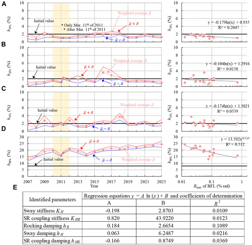
FIGURE 10. Aging and amplitude dependence of damping for superstructure, and regression equations for other physical parameters. (A) Damping of 3FL. (B) Damping of 2FL. (C) Damping of 1FL. (D) Damping of BFL. (E) Amplitude dependence of identified parameters not subject to evaluation.

Figures 10A–C reveal no significant changes in the damping characteristics of superstructure attributed to aging. Furthermore, no apparent variation in the damping constant due to amplitude dependence is observed. In years with large fluctuations, the variance of the identified parameters is also large, suggesting a decline in estimation accuracy. In addition, the variation remains at approximately 1%–2%, consistent with the statistical value from the existing RC structure database (Architectural Institute of Japan, 2020). The damping constant h_BFL of the BI layer shown in Figure 10D decreases as the average maximum inter-story deformation angle increases, in the same manner of its stiffness. This amplitude dependence is considered to be the cause of yearly fluctuations in the attenuation constant. The mechanism through which the attenuation constant decreases depending on the amplitude is considered to be as follows. The standard value of a damping force F_D of the viscous damper of the BI building is proportional to the 0.4–1.0 power of the velocity v, which is expressed in Eqs 22a, b (Tanaka et al., 2018). However, because the analytical model used for identification is a linear model in the frequency domain, the damping force ${\stackrel{\sim }{F}}_D$ is expressed by Eq. 23. Subsequently, by contrasting Eqs 22a, b), and (Eq. 23) with the relationship between the damping constant and damping coefficient, we obtain Eq. 24. According to this equation, the damping constant decreases as the amplitude increases. This velocity amplitude-dependent characteristic can be presumed also to have affected the damping constant shown in Figure 10D.

$F_D=\alpha e^{-0.043t}{\left(0.01v/10\right)}^{\beta }=C{v}^{\beta },(\mathrm{22a})$

$\beta =\left\{\begin{array}{l}1.0\left(v<0.1\text{cm}/\mathrm{s}\right)\\ 0.59\left(0.1\text{\hspace{0.17em}cm}/\mathrm{s}\le v<1.0\text{cm}/\mathrm{s}\right)\\ 0.4\left(1.0\text{\hspace{0.17em}cm}/\mathrm{s}\le v\right)\end{array}\right.,(\mathrm{22b})$

${\stackrel{\sim }{F}}_D=\stackrel{\sim }{C}v,(23)$

$h=\stackrel{\sim }{C}/C_c=C{v}^{\beta -1}/C_c,(24)$

where α is a constant depending on the velocity v, t is the temperature, β is a power exponent depending on v, and C_c is the critical damping coefficient.

The above results demonstrate that no significant decrease in stiffness or change in attenuation occurs due to aging in each physical parameter, excluding the BI layer, and no damage due to earthquake motion is estimated. Moreover, no clear tendency is observed in the amplitude dependence of these parameters. Considering the results of the numerical experiments in Section 3, the fluctuations other than those of the seismic isolation layer are thought to be due to the instability of the identification accuracy associated with the spectral characteristics of seismic motion. For the BI layer, clear amplitude dependence in the stiffness and damping constant was confirmed. The tendency for the stiffness to decrease with amplitude corresponds well with the previous research results, such as those for high-damping rubber. On the contrary, the tendency for the damping to decrease depending on the amplitude is the opposite of the amplitude dependence caused by high-damping rubber. This finding is inferred to be due to the properties of the viscous damper installed in the building. As the amplitude dependence of seismically isolated buildings differs depending on the seismic isolation system adopted, as much data as possible should be collected in the future.

No clear aging or amplitude dependence was observed for the rocking soil spring either. However, the ambiguity of the dominant response of the target transfer function likely affected the identification results, especially for the rocking soil spring. This aspect represents a limitation of the accuracy of the single-point fitting of the transfer function proposed in this study. Furthermore, the process used to extract the dominant reactions visually in the proposed framework should be improved.

4.4 Observation record simulation considering amplitude dependence

Finally, a seismic response analysis of representative seismic waves from 2007 to 2023 using the physical parameters identified using the mass point system model was performed, and the effectiveness of the parameter evaluation results was confirmed by comparing the responses with the observation records. Considering the results presented in the previous section, the physical parameters were evaluated using the regression equations of the amplitude dependence shown in Figures 9, 10. The amplitude adopted to the regression equation to estimate each physical parameter was determined from the maximum inter-story deformation angle of each earthquake motion. In the seismic response analysis, the horizontal acceleration response in the observation record of the BFL mass point was used as the forced acceleration. The earthquake motions to be conducted were the following six waves, which had different amplitude levels: the 2011 Tohoku Earthquake and the aftershocks on the same day (the maximum inter-story deformation angles of BFL, R_max = 5.56% and 1.93% rad, were defined as the mainshock and aftershock, respectively); the 2008 and 2022 earthquakes, in which the inter-story deformation angle of the BFL was maximum between 2007 and 2010 or 2012 and 2023 (R_max = 0.27% and 0.88% rad for BFL, respectively); and the 2007 and 2023 earthquakes with small amplitude levels (R_max = 0.05% and 0.02% rad for BFL, respectively), totaling six waves.

Figures 11A–F show the maximum response distribution along the height direction based on the analysis performed using the identified physical parameters. The upper row depicts the absolute acceleration, and the lower presents the displacement relative to the BFL. The results based on the initial values (Ini.) and observation records (Obs.) are also provided in the same images. Figures 11A–F demonstrate that the maximum acceleration and relative displacement are consistent with the observation records. The consistency of the responses is also higher than that of the initial values. The initial stiffness of the BI layer based on the seismic design was assumed to be 40% of the shear strain, and the strain level of the evaluated ground motions was lower than that assumed in the design. Therefore, the identification results considering the amplitude dependence exhibited better consistency.

FIGURE 11

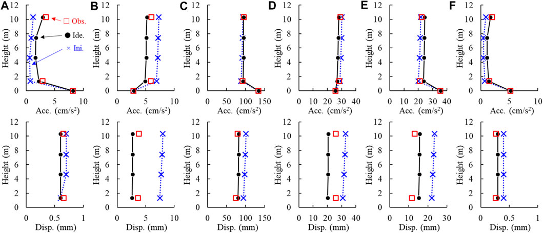
FIGURE 11. Comparison of maximum response values between initial value, identification, and observation (bottom: relative displacement to BFL, top: acceleration). (A) R_max: 0.05% rad in 2007. (B) R_max: 0.27% rad in 2008. (C) R_max: 5.56% rad in mainshock of 11/03/2011. (D) R_max: 1.93% rad in aftershock of 11/03/2011. (E) R_max: 0.88% rad in 2022. (F) R_max: 0.02% rad in 2023.

Figures 12A–F present the acceleration response spectra (h = 5%) in the horizontal directions of RFL and 1FL and the rocking direction of BFL obtained from observation (Obs.) and analysis (Identification parameter: Ide. or initial value: Ini.) for six representative waves, arranged chronologically from 2007 onward. The responses of RFL and 1FL in Figures 12A–F show that the dominant responses around 1.0–2.0 s agree well between the analysis based on identified parameters and observation results. In Figures 12A, E, F, the response around 0.1–0.2 s, which is the second-order mode, also agrees between the observation and analysis results. The rocking responses of BFL in Figures 12A–F demonstrate that higher-order peaks more than 0.1 s were reproduced in the analysis based on the identification results, whereas the amplitude was underestimated.

FIGURE 12

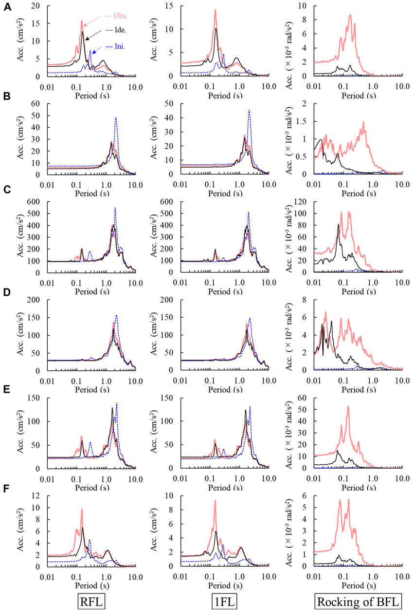
FIGURE 12. Comparison of acceleration response spectrum (h = 5%) between initial value, identification, and observation for six seismic motions (from left to right: RFL, 1FL, and rocking of BFL). (A) 2007. (B) 2008. (C) Mainshock of 2011 Tohoku Earthquake. (D) Aftershock of 2011 Tohoku Earthquake. (E) 2022. (F) 2023.

The above results confirm that the response reproducibility was improved by identifying physical parameters considering higher-order modes using the proposed method. In addition, the regression results for physical parameters based on the assumed amplitude dependence described in the previous section can explain building responses to earthquake motions of different amplitude levels.

5 Conclusion and future works

In this study, to evaluate the soundness of superstructures and foundations using limited superstructure observation data without ground responses, we proposed an efficient framework for identifying physical parameters by considering higher-order modes. We applied the MIEC method to the proposed framework and verified the effectiveness of the method. First, the effectiveness of the proposed method was confirmed through numerical experiments. The physical parameters were then identified for the observation record of an actual BI building, and an observation record simulation was performed using the identified parameters. The findings of this study can be summarized as follows:

1) The numerical experiments confirmed that the proposed framework could effectively estimate the stiffness and damping of superstructures and dynamic soil springs in the sway and rocking directions. In particular, the stiffness estimation of each part exhibited good accuracy, with an error of approximately 10% when subjected to white noise excitation. Consequently, the applicability of the proposed method to the SHM of the superstructure and the indirect monitoring of the soil and foundation was confirmed. However, the findings also confirmed that when the decrease in stiffness due to foundation damage or the dissipative damping of the ground or both are large, the identification accuracy of physical parameters may decrease. In particular, if higher-order modes are not excited due to the spectral characteristics of seismic motion, the accuracy of parameter identification tends to decrease. These points indicate the limitations of the current accuracy of this method and lead to the following important suggestions. First, higher-order modes should be considered and captured to identify the physical parameters of not only the superstructure, but also dynamic soil springs in BI buildings. The estimation accuracy of the physical parameters may decrease because the proposed method uses only the dominant response of each single point in the transfer function fitting. The reproducibility of the shape of the transfer function parabola may be important for the estimation both of stiffness and damping characteristics. In addition, the SR-coupled spring, treated as an arbitrary external force, was not evaluated correctly. These are the current limitations and future challenges of the proposed method.

2) We applied our proposed method to long-term observation records, including those both before and after the 2011 Tohoku Earthquake, of an actual BI building. No significant decrease in stiffness or change in attenuation due to aging was observed, nor was any amplitude dependence evident for any physical parameter, except in the BI layer. Considering the results of the numerical experiments, the parameter fluctuations are due to the instability of the identification accuracy associated with the spectral characteristics of seismic motion. For the BI layer, clear amplitude dependence was confirmed in the stiffness and damping constant. The tendency for the stiffness to decrease with amplitude corresponds well with previous research results, such as those for high-damping rubber (Morii et al., 2015). On the contrary, the tendency for the damping to decrease depending on amplitude is the opposite of the amplitude dependence caused by high-damping rubber. As the amplitude dependence of BI buildings differs depending on the seismic isolation system adopted, as much data as possible should be collected in the future. No clear aging or amplitude dependence was observed in the rocking soil spring either. The above results indicate that no structural damage was caused to either the superstructure or soil and foundations. However, the ambiguity of the dominant response of the target transfer function likely affected the identification results, especially for the soil spring. This aspect limits the accuracy of the single-point fitting of the transfer function proposed in this article. Furthermore, the process of visually extracting the dominant mode in the proposed framework should be improved.

3) The observation simulation analysis of SR model confirmed that the response reproducibility was improved by identifying physical parameters considering modes of higher orders using the proposed method. In addition, we found that the regression results of physical parameters based on the amplitude dependence could explain building responses to six earthquake motions of different amplitude levels. These results suggest that using the proposed physical parameter identification framework can be expected to confirm the validity of seismic design models and improve safety against seismic responses.

In the future, we plan to study methods of efficiently extracting the dominant response of the transfer function, including the envelope shape. We will also extend the proposed framework to more complex problems, such as three-dimensional analysis.

Data availability statement

The data analyzed in this study is subject to the following licenses/restrictions: The datasets presented in this article are not readily available because due to the nature of this research, the owner of subjected building of this study did not agree for their data to be shared publicly, so supporting data is not available. Requests to access these datasets should be directed to TT, toujou.takaki@takenaka.co.jp.

Author contributions

TT: Conceptualization, Formal Analysis, Methodology, Validation, Visualization, Writing–original draft. TS: Formal Analysis, Writing–review and editing. SN: Conceptualization, Supervision, Writing–review and editing.

Funding

The author(s) declare that no financial support was received for the research, authorship, and/or publication of this article.

Acknowledgments

We thank Mr. Takayuki Sone, Dr. Hideo Kyuke, and Mr. Shuei Ikeda of Takenaka Corporation for their help in collecting the specifications and observation records of the buildings used in this research. We also thank Dr. Takanori Hida, Associate Professor at Ibaraki University, for his valuable advice regarding our research. We would like to thank Editage (www.editage.jp) for English language editing.

Conflict of interest

Authors TT and TS were employed by Takenaka Corporation.

The remaining author declares that the research was conducted in the absence of any commercial or financial relationships that could be construed as a potential conflict of interest.

Publisher’s note

All claims expressed in this article are solely those of the authors and do not necessarily represent those of their affiliated organizations, or those of the publisher, the editors and the reviewers. Any product that may be evaluated in this article, or claim that may be made by its manufacturer, is not guaranteed or endorsed by the publisher.

References

Architectural Institute of Japan (1987). Seismic loading: state of the art and future developments.

Google Scholar

Architectural Institute of Japan (2006). Seismic response analysis and design of buildings considering dynamic soil-structure interaction.

Google Scholar

Architectural Institute of Japan (2020). Damping and vibration of buildings.

Google Scholar

Astroza, R., Conte, P. J., Restrepo, I. J., Ebrahimian, H., and Hutchinson, T. (2021). Seismic response analysis and modal identification of a full-scale five-story base-isolated building tested on the NEES@UCSD shake table. Eng. Struct. 238, 112087. doi:10.1016/j.engstruct.2021.112087

CrossRef Full Text | Google Scholar

Byung, K. O., Kyu, J. K., Yousok, K., Hyo, S. P., and Hojjat, A. (2017). Evolutionary learning based sustainable strain sensing model for structural health monitoring of high-rise buildings. Appl. Soft Comput. J. 58, 576–585. doi:10.1016/j.asoc.2017.05.029

CrossRef Full Text | Google Scholar

Chen, T., Morris, J., and Martin, E. (2005). Particle filters for state and parameter estimation in batch processes. J. Process Control. 15, 665–673. doi:10.1016/j.jprocont.2005.01.001

CrossRef Full Text | Google Scholar

Cristina, M., Juan, J. A., Luis, H. P., and Orlando, M. (2013). Effects of soil-structure interaction on the dynamic properties and seismic response of piled structures. Soil Dyn. Earthq. Eng. 53, 160–175. doi:10.1016/j.soildyn.2013.07.004

CrossRef Full Text | Google Scholar

Cruz, C., and Miranda, E. (2021). Insights into damping ratios in buildings. Earthq. Eng. Struct. Dyn. 50, 916–934. doi:10.1002/eqe.3356

CrossRef Full Text | Google Scholar

Fujita, K., and Takewaki, I. (2018). Stiffness identification of high-rise buildings based on statistical model-updating Approach. Front. Built Environ. 4, 9. doi:10.3389/fbuil.2018.00009

CrossRef Full Text | Google Scholar

Furukawa, T., Ito, M., Izawa, K., and Noori, N. M. (2005). System identification of base-isolated building using seismic response data. J. Eng. Mech. 131, 268–275. doi:10.1061/(ASCE)0733-9399(2005)131:3(268)

CrossRef Full Text | Google Scholar

Hamaguchi, H., Aizawa, S., Samejima, Y., Kikuchi, T., Suzuki, S., and Yoshizawa, T. (2009). A study of aging effect on a rubber bearing after about twenty years in use. AIJ J. Technol. Des. 15, 393–398. doi:10.3130/aijt.15.393

CrossRef Full Text | Google Scholar

Hamaguchi, H., and Sasaki, K. (2009). “A study of aging effect on a liquid material for viscous dampers after about twenty years in use,” in Summaries of technical papers of annual meeting (Tokyo, Japan: Architectural Institute of Japan), 859–860.

Google Scholar

Hamaguchi, H., and Yamamoto, M. (2005). “Damping effect of viscous damper under micro vibration,” in Summaries of technical papers of annual meeting (Tokyo, Japan: Architectural Institute of Japan), 839–840.

Google Scholar

Hamamoto, T., Choi, J., and Shimizu, M. (2010). Experiment verification for indirect health monitoring of pile foundations. J. Struct. Constr. Eng. Trans. AIJ. 75, 1445–1454. doi:10.3130/aijs.75.1445

CrossRef Full Text | Google Scholar

Hayashi, K., Hachimorim, W., Kaneda, S., Tamura, S., and Saito, T. (2017). Development of the monitoring technique on the damage of piles using the biggest shaking table “E-Defense”. AIP Conf. Proc. 1892, 020015. doi:10.1063/1.5005646

CrossRef Full Text | Google Scholar

Hernandez, F., Diaz, P., Astroza, R., Ochoa-Cornejo, F., and Zhang, X. (2021). Time variant system identification of superstructures of base-isolated buildings. Eng. Struct. 246, 112697. doi:10.1016/j.engstruct.2021.112697

CrossRef Full Text | Google Scholar

Higashino, M., Aizawa, S., Yoneda, G., Yoshizawa, T., and Sueyasu, T. (1997). “A study of aging effect on a rubber bearing after 10 years in use,” in Summaries of technical papers of annual meeting (Tokyo, Japan: Architectural Institute of Japan).

Google Scholar

Hoshiya, M., and Saito, E. (1984). Structural identification by extended Kalman filter. J. Eng. Mech. 110, 1757–1770. doi:10.1061/(ASCE)0733-9399(1984)110:12(1757)

CrossRef Full Text | Google Scholar

Jabini, A., Mahsuli, M., and Ghahari, F. S. (2018). Probabilistic blind identification of soil-structure systems using extended Kalman filter. Proceedings of the 11th National Conference in Earthquake Engineering. Los Angeles, CA. Earthquake Engineering Research Institute.

Google Scholar

The Building Center of Japan. (1992). The building center of Japan. https://www.bcj.or.jp/download/wave/ (Accessed December 21, 2023).

Google Scholar

Kamoshita, N., Hamaguchi, H., Tani, Y., and Suzuki, S. (2018). A study of aging effect on a rubber bearing after about thirty years in use. AIJ J. Technol. Des. 24, 41–46. doi:10.3130/aijt.24.41

CrossRef Full Text | Google Scholar

Kikitsu, H., Mukai, T., Kato, H., Hirade, T., Hasegawa, T., Kahiwa, H., et al. (2017). Analysis of the barrier to post-seismic continuous usability of buildings and proposal of the related performance requirement. AIJ J. Technol. Des. 23, 331–336. doi:10.3130/aijt.23.331

CrossRef Full Text | Google Scholar

Kyuuke, H., Yamamoto, M., and Higashino, M. (2005). Earthquake observation records of the chikuyu-ryou of takenaka corp. during the earthquake of northwest of chiba prefecture. MENSHIN 50, 44–45.

Google Scholar

Limongelli, M. P., and Çelebi, M. (2019). Seismic structural health monitoring—from theory to successful applications. Berlin, Germany: Springer Tracts in Civil Engineering.

Google Scholar

Morii, T., Takeuchi, S., Yoshida, K., Saruta, M., and Adachi, K. (2015). Effect of equivalent stiffness of seismic isolation device on environmental vibration assessment. AIJ J. Technol. Des. 21, 1101–1105. doi:10.3130/aijt.21.1101

CrossRef Full Text | Google Scholar

National Research Institute for Earth Science and Disaster Resilience (2019). NIED K-net, KiK-net. doi:10.17598/NIED.0004

CrossRef Full Text | Google Scholar

Safak, E. (1991). Identification of linear structures using discrete-time filters. J. Struct. Eng. 117, 3064–3085. doi:10.1061/(ASCE)0733-9445(1991)117:10(3064)

CrossRef Full Text | Google Scholar

Shinagawa, Y., and Mita, A. (2013). Estimation of earthquake response of a building using an accelerometer. AIJ J. Technol. Des. 19, 461–464. doi:10.3130/aijt.19.461

CrossRef Full Text | Google Scholar

Shirzad-Ghaleroudkhani, N., Mahsuli, M., Ghahari, S. F., and Taciroglu, E. (2017). Bayesian identification of soil–foundation stiffness of building structures. Struct. Control Health Monit. 25, e2090. doi:10.1002/stc.2090

CrossRef Full Text | Google Scholar

Suzuki, T. (2018). Input motion inversion in elasto-plastic soil model by using modal iterative error correction method. J. Struct. Constr. Eng. Trans. AIJ. 83, 1021–1029. doi:10.3130/aijs.83.1021

CrossRef Full Text | Google Scholar

Suzuki, T. (2019). Mode selection method in modal iterative error correction for stabilization of convergence. J. Struct. Constr. Eng. Trans. AIJ. 84, 195–203. doi:10.3130/aijs.84.195

CrossRef Full Text | Google Scholar

Suzuki, T., and Tojo, T. (2020). Identification of rotational input motion and damping ratio using horizontal acceleration records. J. Struct. Constr. Eng. Trans. AIJ. 85, 51–60. doi:10.3130/aijs.85.51

CrossRef Full Text | Google Scholar

Suzuki, Y., and Mita, A. (2016). Output only estimation of inter-story drift angle for buildings using small number of accelerometers. J. Struct. Constr. Eng. Trans. AIJ. 81, 1061–1070. doi:10.3130/aijs.81.1061

CrossRef Full Text | Google Scholar

Tajimi, H., and Shimomura, Y. (1976). Dynamic analysis of soil-structure interaction by the thin layered element method. Trans. AIJ. 243, 41–51. doi:10.3130/aijsaxx.243.0_41

CrossRef Full Text | Google Scholar

Tanaka, G., Kinoshita, T., and Hamaguchi, H. (2018). “A study of aging effect on a liquid material for viscous dampers after about thirty years in use,” in Summaries of technical papers of annual meeting (Tokyo, Japan: Architectural Institute of Japan), 1003–1004.

Google Scholar

Terazawa, Y., and Takeuchi, T. (2018). Optimal damper design strategy for braced structures based on generalized response spectrum analysis. J. Struct. Constr. Eng. Trans. AIJ. 83, 1689–1699. doi:10.3130/aijs.83.1689

CrossRef Full Text | Google Scholar

Tojo, T., and Nakai, S. (2022). Identification of sway rocking springs and pile damage detection using subspace method. J. Struct. Constr. Eng. Trans. AIJ. 87, 60–71. doi:10.3130/aijs.87.60

CrossRef Full Text | Google Scholar

Tojo, T., Nakamura, N., and Nabeshima, K. (2023). Evaluation of vibration characteristics of RC buildings considering dynamic soil-structure interaction based on large shaking table test. J. Struct. Constr. Eng. Trans. AIJ. 88, 920–931. doi:10.3130/aijs.88.920

CrossRef Full Text | Google Scholar

Uesaka, T., Nabeshima, K., Nakamura, N., and Suzuki, T. (2021b). Physical parameters identification for full-scale ten-story reinforced concrete building with degrading tri-linear model by modal iterative error correction method. Earthq. Eng. Struct. Dyn. 51, 153–168. doi:10.1002/eqe.3560

CrossRef Full Text | Google Scholar

Uesaka, T., Nakamura, N., and Suzuki, T. (2021a). Parameter identification for nonlinear structural model using modal iterative error correction method. Eng. Struct. 232, 111805. doi:10.1016/j.engstruct.2020.111805

CrossRef Full Text | Google Scholar

Verhaegen, M. (1993). Subspace model identification Part 3. Analysis of the ordinary output-error state-space model identification algorithm. Int. J. Control. 58, 555–586. doi:10.1080/00207179308923017

CrossRef Full Text | Google Scholar

Yamamoto, M. (2011). Evaluations of seismically isolated buildings based on observed records. Takenaka Technical Report. No. 67.

Google Scholar

Yu, T., Johnson, A. E., Brewick, T. P., Christenson, E. R., Sato, E., and Sasaki, T. (2023). Modeling and model updating of a full-scale experimental base-isolated building. Eng. Struct. 280, 114216. doi:10.1016/j.engstruct.2022.114216

CrossRef Full Text | Google Scholar

Zhang, M., Guo, T., Zhu, R., Zong, Y., Liu, Z., and Xu, W. (2023). Damage identification of seismic-isolated structure based on CAE network using vibration monitoring data. Eng. Struct. 283, 115873. doi:10.1016/j.engstruct.2023.115873

CrossRef Full Text | Google Scholar