Fishbone model-based inversion to estimate physical parameters of elastic structures under earthquake excitations

This study established an inversion based on a fishbone model to estimate physical parameters from the responses of elastic building structures subjected to an earthquake. A fishbone model, which has rotational springs and dashpots in addition to the elements in a lumped mass model, is effective for demonstrating structural rotations that happen at the connections of columns and beams. This model is commonly applied to computational calculations of seismic responses of structures and is classified into a forward problem obtaining responses from known systems and excitations. Although its effectiveness for the forward problem has been well demonstrated, it has rarely been applied to the inverse problem, where structural properties are estimated from known responses and excitations. First, this study inverted multi/single-mass-system fishbone models. Then, the inversion was applied to an elastic fishbone model of a 3-mass system, which was built based on an E-Defense shaking table experiment, and its structural responses were numerically simulated. This numerical simulation demonstrated its effectiveness for accurately estimating parameters in the fishbone model of the 3-mass system, especially when its structural responses are not contaminated by noises. Lastly, it was applied to responses containing some noise to examine its influence on the estimation accuracy. The estimation accuracy of damping elements was found to be sensitive to noise, whereas that of stiffness was more insensitive than the damping elements. The proposed inversion is particularly suitable for estimating rotational stiffness, which is not obtainable from the inversion of lumped mass systems.

1 Introduction

Structural health monitoring is an important subject for maintenance of systems in various fields, such as aerospace and mechanical and civil engineering (Farrar and Worden 2006). Monitoring is basically expected to find abnormalities (e.g., damage) within the systems, as well as more detailed local information such as damage location and severity (Chang et al., 2003). Although the location is fundamental information for damage restoration, the severity directly affects the operation, because it is closely related to safety management.

Abnormalities are more frequently observed after natural disasters, such as earthquakes, than during normal times (Sohn et al., 2001), (Brownjohn 2007). In fact, during the Great East Japan Earthquake of 2011, millions of buildings and structures in distributed over a wide area were severely shaken by the huge earthquake. Afterward, there was a significant demand for post-earthquake condition assessments to ensure structural integrity against subsequent aftershocks (Fujino et al., 2019).

Visual inspection by humans is a direct approach for assessment, although its accuracy greatly relies on the capability of the inspectors as well as the visibility and accessibility of the damage (Nagarajaiah and Yang 2017). However, such inspections are problematic, especially in post-earthquake situations, because they require inspectors to enter the buildings or access structures whose safety is unsecured, sometimes with a high possibility of similar or even larger earthquakes. On top of that, after a large earthquake, inspections are difficult to obtain due to the scarcity of labor and electricity, as well as the price increases caused by the lack of various products (Lynch 2007). Thus, structural assessment after disasters must be freed from the need for human effort and performed in a systematic way to smoothly deal with a huge number of structures. Therefore, structural health monitoring based on structural vibration data is a promising approach (Nagarajaiah and Yang 2017), (Balsamo and Betti 2015), because it uses data automatically acquired by sensors attached to structures for the assessment. Currently, the development of efficient structural monitoring techniques for the seismic damage detection based on structural responses is active and an important subject in earthquake engineering.

The modal information for structures (i.e., natural frequencies, their corresponding damping ratios, and modal shapes) has been commonly used as indices to find abnormalities (Brownjohn 2007); (Hearn and Testa 1991); (Doebling et al., 1996); (Ji et al., 2011); (Iiyama et al., 2015); (Fujiwara et al., 2021), and it is extensively used for systems having time-varying parameters (Tobita 1996); (Moaveni and Asgarieh 2012); (Astroza et al., 2018); (Li and Law 2009). However, the modal information of a structure is governed by its entire condition and insensitive to local structural damage, such as fractures or cracks in beams (Xie et al., 2018). Thus, assessments based on the modal information in general have difficulties in obtaining detailed local information.

In response to the need for local information from the assessment, much attention has been recently paid to approaches that directly estimate physical parameters of structures (i.e., mass, damping, and stiffness) rather than the modal information (Kang et al., 2005), (Kuleli and Nagayama 2019). In this regard, a time domain inversion (TDI), which selects suitable parameters for an assumed model by the least squares method and time history structural responses (i.e., acceleration, velocity, and displacement), has been a useful approach, particularly for linear systems or those with little parameter variation (Agbabian et al., 1991); (Nakamura and Yasui 1999); (Shintani, Yoshitomi, and Takewaki 2017). However, regarding nonlinear systems, TDI has been mainly used for the estimation of the nonlinear restoring force within a system (Toussi and Yao 1983); (Masri et al., 1987(a)); (Masri et al., 1987(b)); (Shintani, Yoshitomi, and Takewaki 2020), rather than those physical parameters. This is mainly attributed to a feature of TDI: it requires enough sampling steps for the estimation, indicating its unsuitability for the exact identification of time-varying parameters.

To address the issue of estimating physical parameters in a nonlinear structure, we have developed simple piecewise linearization in time series (SPLiTS) (Enokida and Kajiwara 2020), for use with TDI. It enables us to estimate the physical parameters in a nonlinear structure by the piecewise linearization of the structure based on half cyclic waves of its displacement responses. Due to the linearization, SPLiTS describes the time-varying stiffness and damping as time history data. The current SPLiTS was specifically developed for a mass-spring-dashpot model that allows only lateral movement. This model is particularly suitable for evaluating structures whose floors, consisting of beams and slabs, are rigid or much stiffer than the columns. However, many actual structures do not satisfy the minimum conditions for SPLiTS, and they require a model that considers the influence of columns and floors separately for more precise modeling. Parameter estimation based on such a detailed model would allow more accurate assessments with more detailed local information.

A fishbone model (Ogawa et al., 1999); (Nakashima et al., 2002), which is constructed as an extension of the mass-spring-dashpot model, has additional elements to simulate structural rotations, which typically occur at connections of columns and beams. The fishbone model was originally developed for numerical analysis of structures to study the seismic response more elaborately than is possible with the mass-spring-dashpot model. Although the model has been occasionally used in system identification tests or damage assessment of structures (Ji et al., 2011); (Soma et al., 2016), physical parameter estimation based on its inversion has not yet been established. This is mainly because the inversion requires the structural rotation response, which has been rarely measured even in laboratory experiments. However, due to advances in measurement devices, such as micro-electromechanical systems, structural dynamic rotation can be more easily measured than before. This indicates the possibility of employing such data for structural monitoring techniques.

Within this context, this study established an inversion based on a fishbone model to estimate physical parameters of elastic building structures subjected to earthquake excitations, aiming for its application to SPLiTS in the future.

The remainder of this manuscript is as follows. Section 2 introduces the inverse problem of a multi-mass system fishbone model. Numerical simulation of the E-Defense testing of a 3-story steel structure and physical parameter estimation based on TDI using an elastic fishbone model of a 3-mass system were conducted. Section 3 introduces the inverse problem of an elastic fishbone model of a single-mass system, and describes physical parameter estimation based on TDI using the single-mass system model. Section 4 introduces physical parameter estimation based on TDI with noise using elastic fishbone models of the 3-mass system and single-mass system. Section 5 compares physical parameter estimation based on TDI using mass-spring-dashpot models of the 3-mass system and single-mass system. Section 6 summarizes the conclusions obtained in this study.

2 Fishbone model of multi-mass system

2.1 Inverse problem of multi-mass system fishbone model

The equations of motion for an n-mass system fishbone model with the foundation fixed, shown in Figure 1, are Eqs 2.1a and 2.1b solved simultaneously with damping neglected (Soma et al., 2016). The derivation process is shown in Supplementary Appendix SA1.

${\mathbf{H}}_1\mathbf{M}\left(\ddot{\mathbf{x}}+\ddot{\mathbf{u}}\right)={\mathrm{\alpha }}_{\mathrm{k}}\mathrm{\theta }\iff \begin{array}{l}\left[\begin{array}{cccccc}{h}_1& h_1+2h_2& h_1+2h_2+2h_3& \cdots & h_1+2h_2+2h_3+\cdots +2h_{n-1}& h_1+2h_2+2h_3+\cdots +2h_{n-1}+2h_n\\ 0& h_2& h_2+2h_3& \cdots & h_2+2h_3+\cdots +2h_{n-1}& h_2+2h_3+\cdots +2h_{n-1}+2h_n\\ 0& 0& h_3& \cdots & h_3+\cdots +2h_{n-1}& h_3+\cdots +2h_{n-1}+2h_n\\ ⋮& ⋮& ⋮& \ddots & ⋮& ⋮\\ 0& 0& 0& \cdots & h_{n-1}& h_{n-1}+2h_n\\ 0& 0& 0& \cdots & 0& h_n\end{array}\right]\times \left\{\begin{array}{c}{m}_1\left({\ddot{x}}_1+\ddot{u}\right)\\ m_2\left({\ddot{x}}_2+\ddot{u}\right)\\ m_3\left({\ddot{x}}_3+\ddot{u}\right)\\ ⋮\\ m_{n-1}\left({\ddot{x}}_{n-1}+\ddot{u}\right)\\ m_n\left({\ddot{x}}_n+\ddot{u}\right)\end{array}\right\}\\ =\left[\begin{array}{cccccc}2k_{B1}+d_1& 2k_{B2}& 2k_{B3}& \cdots & 2k_{Bn-1}& 2k_{Bn}\\ -d_2& 2k_{B2}+d_2& 2k_{B3}& \cdots & 2k_{Bn-1}& 2k_{Bn}\\ 0& -d_3& 2k_{B3}+d_3& \cdots & 2k_{Bn-1}& 2k_{Bn}\\ ⋮& ⋮& ⋮& \ddots & ⋮& ⋮\\ 0& 0& 0& \cdots & 2k_{Bn-1}+d_{n-1}& 2k_{Bn}\\ 0& 0& 0& \cdots & -d_n& 2k_{Bn}+d_n\end{array}\right]\left\{\begin{array}{c}{\theta }_1\\ {\theta }_2\\ {\theta }_3\\ ⋮\\ {\theta }_{n-1}\\ {\theta }_n\end{array}\right\}\end{array}$(2.1a)

${\mathbf{H}}_2\mathbf{M}\left(\ddot{\mathbf{x}}+\ddot{\mathbf{u}}\right)={\mathrm{\beta }}_{\mathrm{k}}\mathrm{\theta }+{\mathbf{E}}_{\mathrm{I}}\mathbf{x}\iff \begin{array}{l}\left[\begin{array}{cccccc}{h}_1& h_1+3h_2& h_1+3h_2+3h_3& \cdots & h_1+3h_2+3h_3+\cdots +3h_{n-1}& h_1+3h_2+3h_3+\cdots +3h_{n-1}+3h_n\\ 0& h_2& h_2+3h_3& \cdots & h_2+3h_3+\cdots +3h_{n-1}& h_2+3h_3+\cdots +3h_{n-1}+3h_n\\ 0& 0& h_3& \cdots & h_3+\cdots +3h_{n-1}& h_3+\cdots +3h_{n-1}+3h_n\\ ⋮& ⋮& ⋮& \ddots & ⋮& ⋮\\ 0& 0& 0& \cdots & h_{n-1}& h_{n-1}+3h_n\\ 0& 0& 0& \cdots & 0& h_n\end{array}\right]\times \left\{\begin{array}{c}{m}_1\left({\ddot{x}}_1+\ddot{u}\right)\\ m_2\left({\ddot{x}}_2+\ddot{u}\right)\\ m_3\left({\ddot{x}}_3+\ddot{u}\right)\\ ⋮\\ m_{n-1}\left({\ddot{x}}_{n-1}+\ddot{u}\right)\\ m_n\left({\ddot{x}}_n+\ddot{u}\right)\end{array}\right\}\\ =\left[\begin{array}{cccccc}3k_{B1}+3d_1& 3k_{B2}& 3k_{B3}& \cdots & 3k_{Bn-1}& 3k_{Bn}\\ 0& 3k_{B2}+3d_2& 3k_{B3}& \cdots & 3k_{Bn-1}& 3k_{Bn}\\ 0& 0& 3k_{B3}+3d_3& \cdots & 3k_{Bn-1}& 3k_{Bn}\\ ⋮& ⋮& ⋮& \ddots & ⋮& ⋮\\ 0& 0& 0& \cdots & 3k_{Bn-1}+3d_{n-1}& 3k_{Bn}\\ 0& 0& 0& \cdots & 0& 3k_{Bn}+3d_n\end{array}\right]\left\{\begin{array}{c}{\theta }_1\\ {\theta }_2\\ {\theta }_3\\ ⋮\\ {\theta }_{n-1}\\ {\theta }_n\end{array}\right\}+\left[\begin{array}{cccccc}{e}_1& 0& 0& \cdots & 0& 0\\ -e_2& e_2& 0& \cdots & 0& 0\\ 0& -e_3& e_3& \cdots & 0& 0\\ ⋮& ⋮& ⋮& \ddots & ⋮& ⋮\\ 0& 0& 0& \cdots & e_{n-1}& 0\\ 0& 0& 0& \cdots & -e_n& e_n\end{array}\right]\left\{\begin{array}{c}{x}_1\\ x_2\\ x_3\\ ⋮\\ x_{n-1}\\ x_n\end{array}\right\}\end{array}$(2.1b)

FIGURE 1

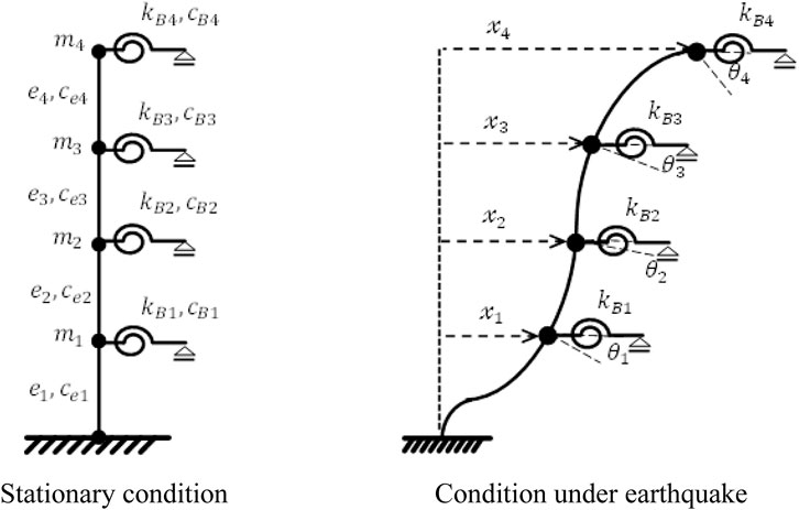
FIGURE 1. Fishbone model of the multi-mass system.

Here, $d_i=\frac{2E{I}_i}{h_i}$, $e_i=\frac{6E{I}_i}{h_i^2}$, $h_i$ is the height of the i-th story, $m_i$ is the mass of the i-th story, $x_i$ is the relative displacement of the i-th story, $\ddot{u}$ is ground acceleration, $k_{Bi}$ is the rotation stiffness of the i-th story, ${\theta }_i$ is the rotation angle of the i-th story beam, and $E{I}_i$ is a coefficient obtained by multiplying the Young’s modulus of the i-th story column by the moment of inertia.

The inverse problem of an n-story fishbone model is formulated by transforming Eq. 2.1b as follows:

$\begin{array}{l}\left[\begin{array}{cccccc}{h}_1\left({\ddot{x}}_1+\ddot{u}\right)& \left(h_1+3h_2\right)\left({\ddot{x}}_2+\ddot{u}\right)& \left(h_1+3h_2+3h_3\right)\left({\ddot{x}}_3+\ddot{u}\right)& \cdots & \left(h_1+3h_2+3h_3+\cdots +3h_{n-1}\right)\left({\ddot{x}}_{n-1}+\ddot{u}\right)& \left(h_1+3h_2+3h_3+\cdots +3h_{n-1}+3h_n\right)\left({\ddot{x}}_n+\ddot{u}\right)\\ 0& h_2\left({\ddot{x}}_2+\ddot{u}\right)& \left(h_2+3h_3\right)\left({\ddot{x}}_3+\ddot{u}\right)& \cdots & \left(h_2+3h_3+\cdots +3h_{n-1}\right)\left({\ddot{x}}_{n-1}+\ddot{u}\right)& \left(h_2+3h_3+\cdots +3h_{n-1}+3h_n\right)\left({\ddot{x}}_n+\ddot{u}\right)\\ 0& 0& h_3\left({\ddot{x}}_3+\ddot{u}\right)& \cdots & \left(h_3+\cdots +3h_{n-1}\right)\left({\ddot{x}}_{n-1}+\ddot{u}\right)& \left(h_3+\cdots +3h_{n-1}+3h_n\right)\left({\ddot{x}}_n+\ddot{u}\right)\\ ⋮& ⋮& ⋮& \ddots & ⋮& ⋮\\ 0& 0& 0& \cdots & h_{n-1}\left({\ddot{x}}_{n-1}+\ddot{u}\right)& \left(h_{n-1}+3h_n\right)\left({\ddot{x}}_n+\ddot{u}\right)\\ 0& 0& 0& \cdots & 0& h_n\left({\ddot{x}}_n+\ddot{u}\right)\end{array}\right]\times \left\{\begin{array}{c}{m}_1\\ m_2\\ m_3\\ ⋮\\ m_{n-1}\\ m_n\end{array}\right\}\\ =\left[\begin{array}{cccccc}3{\theta }_1& 3{\theta }_2& 3{\theta }_3& \cdots & 3{\theta }_{n-1}& 3{\theta }_n\\ 0& 3{\theta }_2& 3{\theta }_3& \cdots & 3{\theta }_{n-1}& 3{\theta }_n\\ 0& 0& 3{\theta }_3& \cdots & 3{\theta }_{n-1}& 3{\theta }_n\\ ⋮& ⋮& ⋮& \ddots & ⋮& ⋮\\ 0& 0& 0& \cdots & 3{\theta }_{n-1}& 3{\theta }_n\\ 0& 0& 0& \cdots & 0& 3{\theta }_n\end{array}\right]\left\{\begin{array}{c}{k}_{B1}\\ k_{B2}\\ k_{B3}\\ ⋮\\ k_{Bn-1}\\ k_{Bn}\end{array}\right\}+\left[\begin{array}{cccccc}{h}_1{\theta }_1+x_1& 0& 0& \cdots & 0& 0\\ 0& h_2{\theta }_2+x_2-x_1& 0& \cdots & 0& 0\\ 0& 0& h_3{\theta }_3+x_3-x_2& \cdots & 0& 0\\ ⋮& ⋮& ⋮& \ddots & ⋮& ⋮\\ 0& 0& 0& \cdots & h_{n-1}{\theta }_{n-1}+x_{n-1}-x_{n-2}& 0\\ 0& 0& 0& \cdots & 0& h_n{\theta }_n+x_n-x_{n-1}\end{array}\right]\left\{\begin{array}{c}{e}_1\\ e_2\\ e_3\\ ⋮\\ e_{n-1}\\ e_n\end{array}\right\}\end{array}$(2.2)

If the mass and height ($m_i$ and $h_i$) of the building and the response values ($x_i$ and ${\theta }_i$) are known, the dynamic characteristics of the building ($k_{Bi}$ and $e_i$) can be evaluated.

2.2 Numerical simulation for E-Defense test of 3-story steel structure

The 3-story steel test specimen used in the E-Defense test in 2013 (ASEBI 2013), (Hyogo Prefecture 2014) is modeled as a fish-bone model. A view of the entire test specimen that was set on the shaking table is shown in Figure 2 (Mizushima et al., 2018).

FIGURE 2

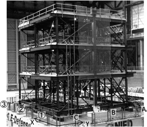
FIGURE 2. 3-story steel test specimen.

2.2.1 Evaluation of elastic stiffness of fishbone column and beam

Elastic stiffness, which is the bending moment at one end of one column and one beam in the i-th story divided by the member angle, is expressed in Eqs 2.3a and 2.3b, respectively (Ogawa et al., 1999).

$K_{Ci}=\frac{1}{\frac{h_i}{6EI}+\frac{2}{G{A}_S{h}_i}},$(2.3a)

$K_{Bi}=\frac{1}{\frac{l}{6EI}+\frac{2}{G{A}_{S}l}+\frac{m}{G{V}_P}},$(2.3b)

where $E$ is Young’s modulus, $I$ is the moment of inertia, $h_i$ is the length of the column, $G$ is the modulus of shear elasticity, $A_S$ is the shear cross-sectional area, $l$ is the length of the beam, $m$ is the number of the beams attached to the panel, and $V_P$ is the volume of the panel.

In our model, a section list of columns and beams for each story is shown in Table 1. The height and weight of each story are shown in Table 2 (Mizushima et al., 2018). The elastic stiffness of the columns in each story was calculated by Eq. 2.3a and tripled because each story has three columns. The elastic stiffness of the beams in each floor was calculated by Eq. 2.3b and I in Eq. 2.3b was doubled because beams are restrained from both sides by the slab. The evaluated elastic stiffness values are shown in Table 3. All the evaluated values were calculated taking the panel size into account.

TABLE 1

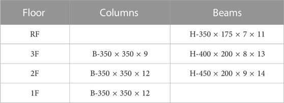
TABLE 1. Section list.

TABLE 2

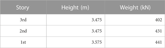
TABLE 2. Heights and weights of specimen.

TABLE 3

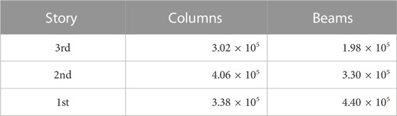
TABLE 3. Evaluated values of elastic stiffness of columns and beams in each story (Unit: kN m).

2.2.2 Comparison of E-Defense test results and elastic fishbone analysis results

The program “fish.f Ver. 2.3” was used for fishbone analysis (Ogawa 2015). The damping was assumed to be proportional to the stiffness matrix, and the damping ratio was set to 2.5%. The beams and columns were set to behave elastically. The base stiffness was set to 1.2 × 10⁵ kN m to match the result in the E-Defense test report (Hyogo Prefecture 2014). The input acceleration was 40% of the intensity of the observed earthquake acceleration at JR Takatori station during the Hanshin-Awaji Earthquake of 1995 (Figure 3). The stress values for members of the test specimen were almost within the elastic range when 40% of the JR Takatori wave was inputted (Mizushima et al., 2018).

FIGURE 3

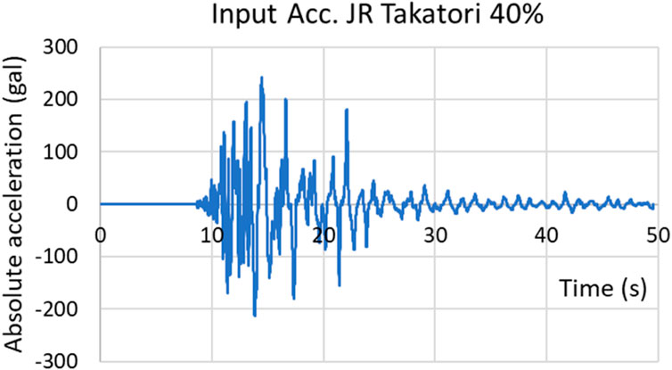
FIGURE 3. Time history wave of input acceleration for 40% of the JR Takatori wave.

The first and second natural frequencies of the specimen and the fishbone analysis model are shown in Table 4. The maximum absolute acceleration values of each floor from the E-Defense test results and the fishbone analysis results are shown in Table 5. The maximum interstory drift values of each story from the E-Defense test results and the fishbone analysis results are shown in Table 6.

TABLE 4

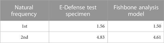
TABLE 4. First and second natural frequencies of specimen and fishbone analysis model (Unit: Hz).

TABLE 5

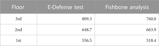
TABLE 5. Maximum absolute accelerations of each floor from E-Defense test results and fishbone analysis results (Unit: cm/s²).

TABLE 6

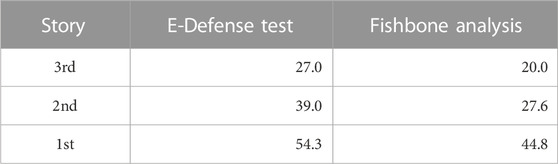
TABLE 6. Maximum interstory drifts of each story from E-Defense test results and fishbone analysis results (Unit: mm).

Figure 4 shows a comparison of time history waves for each story response in the E-Defense test results and fishbone analysis results. Left panels show the time history waves of the absolute acceleration, and right panels show those of the interstory drift. The results show that the fishbone analysis approximately simulates the E-Defense test results.

FIGURE 4

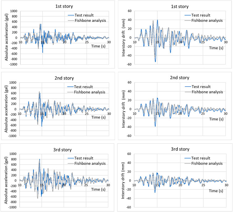
FIGURE 4. Comparison of time history waves from the E-Defense test results and fishbone analysis results for the response of each story.

2.3 Physical parameter estimation for elastic fishbone model of 3-mass system

The terms representing the shear stiffness in Eqs 2.3a and 2.3b, and also the panel term in Eq. 2.3b were neglected after the analysis explained in Section 2.2 because we estimated $e_i$ in Eq. 2.2 for the inverse analysis. The fishbone model of the 3-mass system, including the mass weights and heights, was set based on the test specimen in the 2013 E-Defense test, in the same way as described in Section 2.2.1. The elastic stiffness of the beams and the moment of inertia of all columns in each story are shown in Table 7. The increase of the moment of inertia due to the restraint by the slab was not considered.

TABLE 7

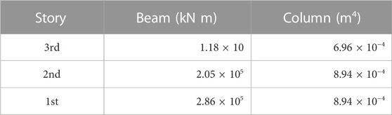
TABLE 7. Elastic stiffness of beams and moment of inertia of all columns in each story for fishbone model.

The damping coefficients for beams and columns were calculated by Eqs 2.4a and 2.4b, respectively.

$c_{Bi}=2h_c{\omega }_1{k}_{Bi},$(2.4a)

$c_{ei}=2h_c{\omega }_1{e}_i,$(2.4b)

where $h_c$ is the damping factor of the superstructure and ${\omega }_1$ is the first natural circular frequency.

These simulations employed the ground motion acceleration recorded by the Japan Meteorological Agency (JMA) during the Hyogo-ken Nanbu/Kobe Earthquake of 1995, and this motion is referred to as the JMA Kobe motion in this study. Figure 5 shows a comparison of time history waves for our forward fishbone analysis results using Eqs 2.1a and 2.1b considering damping proportional to the stiffness and the forward fishbone analysis results using the fish.f program (Ogawa 2015), for each story response, when 10% of the intensity of the JMA Kobe motion was inputted. Our forward fishbone analysis can accurately follow the fish.f program analysis. The damping factor of superstructure $h_c$ was assumed to be 2.5%.

FIGURE 5

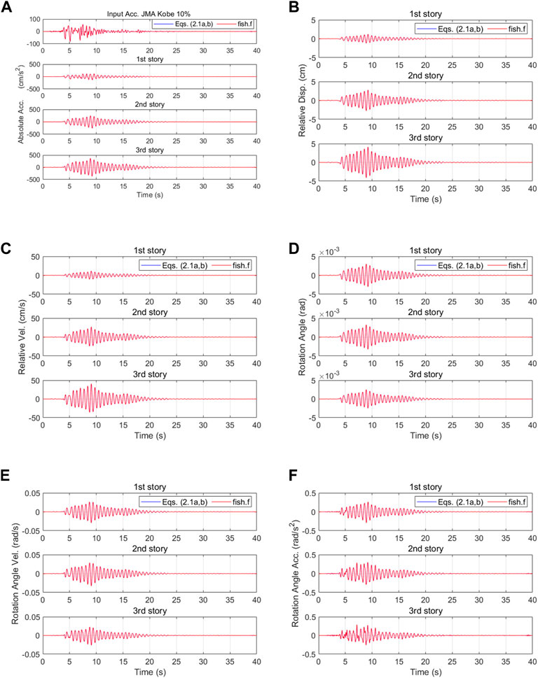
FIGURE 5. Comparison of time history waveforms obtained by our forward fishbone analysis using Eqs 2.1a and 2.1b considering damping proportional to the stiffness and time history waveforms obtained by the fish.f analysis for each story response: (A) absolute acceleration, (B) relative displacement, (C) relative velocity, (D) rotation angle, (E) rotation angle velocity, and (F) rotation angle acceleration.

Eq. 2.2 for a fishbone model of a 3-mass system considering damping proportional to the stiffness is expressed as

$\begin{array}{l}\left[\begin{array}{ccc}{h}_1\left({\ddot{x}}_1+\ddot{u}\right)& \left(h_1+3h_2\right)\left({\ddot{x}}_2+\ddot{u}\right)& \left(h_1+3h_2+3h_3\right)\left({\ddot{x}}_3+\ddot{u}\right)\\ 0& h_2\left({\ddot{x}}_2+\ddot{u}\right)& \left(h_2+3h_3\right)\left({\ddot{x}}_3+\ddot{u}\right)\\ 0& 0& h_3\left({\ddot{x}}_3+\ddot{u}\right)\end{array}\right]\left\{\begin{array}{c}{m}_1\\ m_2\\ m_3\end{array}\right\}\\ =\left[\begin{array}{cccccccccccc}3{\theta }_1& 3{\theta }_2& 3{\theta }_3& 3{\dot{\theta }}_1& 3{\dot{\theta }}_2& 3{\dot{\theta }}_3& h_1{\theta }_1+x_1& 0& 0& h_1{\dot{\theta }}_1+{\dot{x}}_1& 0& 0\\ 0& 3{\theta }_2& 3{\theta }_3& 0& 3{\dot{\theta }}_2& 3{\dot{\theta }}_3& 0& h_2{\theta }_2+x_2-x_1& 0& 0& h_2{\dot{\theta }}_2+{\dot{x}}_2-{\dot{x}}_1& 0\\ 0& 0& 3{\theta }_3& 0& 0& 3{\dot{\theta }}_3& 0& 0& h_3{\theta }_3+x_3-x_2& 0& 0& h_3{\dot{\theta }}_3+{\dot{x}}_3-{\dot{x}}_2\end{array}\right]\times \left\{\begin{array}{c}{k}_{B1}\\ k_{B2}\\ k_{B3}\\ c_{B1}\\ c_{B2}\\ c_{B3}\\ e_1\\ e_2\\ e_3\\ c_{e1}\\ c_{e2}\\ c_{e3}\end{array}\right\},\end{array}$(2.5)

where $c_{Bi}=\alpha k_{Bi}$, $c_{ei}=\beta e_i$, and $\alpha ,\beta$ are proportional coefficients.

When the number of response data for the time history response analysis is $n_d$, Eq. 2.5 can be expressed by

${\mathbf{R}}_{\mathbf{2}}\left\{\begin{array}{c}{m}_1\\ m_2\\ m_3\end{array}\right\}={\mathbf{R}}_1\left\{\begin{array}{c}{k}_{B1}\\ k_{B2}\\ k_{B3}\\ c_{B1}\\ c_{B2}\\ c_{B3}\\ e_1\\ e_2\\ e_3\\ c_{e1}\\ c_{e2}\\ c_{e3}\end{array}\right\},$(2.6)

where

${\mathbf{R}}_{\mathbf{1}}=\left[\begin{array}{cccccccccccc}3{\mathbf{\theta }}_{\mathbf{1}}& 3{\mathbf{\theta }}_{\mathbf{2}}& 3{\mathbf{\theta }}_{\mathbf{3}}& 3{\dot{\mathbf{\theta }}}_{\mathbf{1}}& 3{\dot{\mathbf{\theta }}}_{\mathbf{2}}& 3{\dot{\mathbf{\theta }}}_{\mathbf{3}}& h_1{\mathbf{\theta }}_{\mathbf{1}}+{\mathbf{x}}_{\mathbf{1}}& 0& 0& h_1{\dot{\mathbf{\theta }}}_{\mathbf{1}}+{\dot{\mathbf{x}}}_{\mathbf{1}}& 0& 0\\ 0& 3{\mathbf{\theta }}_{\mathbf{2}}& 3{\mathbf{\theta }}_{\mathbf{3}}& 0& 3{\dot{\mathbf{\theta }}}_{\mathbf{2}}& 3{\dot{\mathbf{\theta }}}_{\mathbf{3}}& 0& h_2{\mathbf{\theta }}_{\mathbf{2}}+{\mathbf{x}}_{\mathbf{2}}-{\mathbf{x}}_{\mathbf{1}}& 0& 0& h_2{\dot{\mathbf{\theta }}}_{\mathbf{2}}+{\dot{\mathbf{x}}}_{\mathbf{2}}-{\dot{\mathbf{x}}}_{\mathbf{1}}& 0\\ 0& 0& 3{\mathbf{\theta }}_{\mathbf{3}}& 0& 0& 3{\dot{\mathbf{\theta }}}_{\mathbf{3}}& 0& 0& h_3{\mathbf{\theta }}_{\mathbf{3}}+{\mathbf{x}}_{\mathbf{3}}-{\mathbf{x}}_{\mathbf{2}}& 0& 0& h_3{\dot{\mathbf{\theta }}}_{\mathbf{3}}+{\dot{\mathbf{x}}}_{\mathbf{3}}-{\dot{\mathbf{x}}}_{\mathbf{2}}\end{array}\right],$(2.7a)

${\mathbf{R}}_{\mathbf{2}}=\left[\begin{array}{ccc}{h}_1\left({\ddot{\mathbf{x}}}_{\mathbf{1}}+\ddot{\mathbf{u}}\right)& \left(h_1+3h_2\right)\left({\ddot{\mathbf{x}}}_{\mathbf{2}}+\ddot{\mathbf{u}}\right)& \left(h_1+3h_2+3h_3\right)\left({\ddot{\mathbf{x}}}_{\mathbf{3}}+\ddot{\mathbf{u}}\right)\\ 0& h_2\left({\ddot{\mathbf{x}}}_{\mathbf{2}}+\ddot{\mathbf{u}}\right)& \left(h_2+3h_3\right)\left({\ddot{\mathbf{x}}}_{\mathbf{3}}+\ddot{\mathbf{u}}\right)\\ 0& 0& h_3\left({\ddot{\mathbf{x}}}_{\mathbf{3}}+\ddot{\mathbf{u}}\right)\end{array}\right],$(2.7b)

in which

${\mathbf{\theta }}_{\mathbf{i}}=\left\{\begin{array}{c}{\theta }_{i1}\\ {\theta }_{i2}\\ ⋮\\ {\theta }_{i{n}_d}\end{array}\right\},{\dot{\mathbf{\theta }}}_{\mathbf{i}}=\left\{\begin{array}{c}{\dot{\theta }}_{i1}\\ {\dot{\theta }}_{i2}\\ ⋮\\ {\dot{\theta }}_{i{n}_d}\end{array}\right\},{\mathbf{x}}_{\mathbf{i}}=\left\{\begin{array}{c}{x}_{i1}\\ x_{i2}\\ ⋮\\ x_{i{n}_d}\end{array}\right\},{\dot{\mathbf{x}}}_{\mathbf{i}}=\left\{\begin{array}{c}{\dot{x}}_{i1}\\ {\dot{x}}_{i2}\\ ⋮\\ {\dot{x}}_{i{n}_d}\end{array}\right\},{\ddot{\mathbf{x}}}_{\mathbf{i}}+\ddot{\mathbf{u}}=\left\{\begin{array}{c}{\ddot{x}}_{i1}+\ddot{u}\\ {\ddot{x}}_{i2}+\ddot{u}\\ ⋮\\ {\ddot{x}}_{i{n}_d}+\ddot{u}\end{array}\right\}\left(i=\mathrm{1,2,3}\right)$

When the number of steps is $n_d\ne 4$, ${\mathbf{R}}_{\mathbf{1}}$ is not a regular matrix, and its direct inversion is infeasible. Thus, instead of the direct solution, the stiffnesses and damping coefficients of beams and columns for the fishbone model of the 3-mass system can be obtained by the pseudo-inversion expressed by

$\left\{\begin{array}{c}{k}_{B1}\\ k_{B2}\\ k_{B3}\\ c_{B1}\\ c_{B2}\\ c_{B3}\\ e_1\\ e_2\\ e_3\\ c_{e1}\\ c_{e2}\\ c_{e3}\end{array}\right\}={\left({{\mathbf{R}}_1}^{\mathrm{T}}{\mathbf{R}}_1\right)}^{-1}{{\mathbf{R}}_1}^{\mathrm{T}}{\mathbf{R}}_{\mathbf{2}}\left\{\begin{array}{c}{m}_1\\ m_2\\ m_3\end{array}\right\}.$(2.8)

TDI, which is a commonly used least squares method for parameter estimations (Toussi and Yao, 1983), is utilized to solve Eq. 2.8. The evaluated values of $k_{Bi}$, $c_{Bi}$, $e_i$, $c_{ei}$ from Eq. 2.8 are exactly equal to the true values of ${\widehat{k}}_{Bi}$, ${\widehat{c}}_{Bi}$, ${\widehat{e}}_i$, ${\widehat{c}}_{ei}$ for all i = 1, 2, 3. When the number of steps is $n_d<4$, the solutions are indeterminate. However, most cases are $n_d>4$.

3 Fishbone model of single-mass system

3.1 Inverse problem of single-mass system fishbone model

The equations of motion for the single-mass system fishbone model with the foundation fixed, shown in Figure 6, are solved simultaneously by Eqs 3.1a and 3.1b when damping proportional to the stiffness is considered.

$h_1{m}_1\left({\ddot{x}}_1+\ddot{u}\right)=\left(2k_{B1}+d_1\right){\theta }_1+\left(2c_{B1}+c_{d1}\right){\dot{\theta }}_1,$(3.1a)

$h_1{m}_1\left({\ddot{x}}_1+\ddot{u}\right)=\left(3k_{B1}+3d_1\right){\theta }_1+e_1{x}_1+\left(3c_{B1}+3c_{d1}\right){\dot{\theta }}_1+c_{e1}{\dot{x}}_1,$(3.1b)

where $c_{di}=\beta d_i$.

FIGURE 6

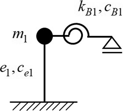
FIGURE 6. Fishbone model of the single-mass system.

The inverse problem of the single-mass system fishbone model is formulated by transforming Eqs 3.1a and 3.1b as follows:

$h_1{m}_1\left({\ddot{x}}_1+\ddot{u}\right)=2{\theta }_1{k}_{B1}+2{\dot{\theta }}_1{c}_{B1}+\frac{h_1{\theta }_1}{3}{e}_1+\frac{h_1{\dot{\theta }}_1}{3}{c}_{e1},$(3.2a)

$h_1{m}_1\left({\ddot{x}}_1+\ddot{u}\right)=3{\theta }_1{k}_{B1}+3{\dot{\theta }}_1{c}_{B1}+\left(h_1{\theta }_1+x_1\right)e_1+\left(h_1{\dot{\theta }}_1+{\dot{x}}_1\right)c_{e1}.$(3.2b)

When the responses of absolute acceleration, relative displacement, relative velocity, rotation angle, and rotation velocity for the fishbone model of the single-mass system are already known, the rotation stiffness and the rotation damping coefficient of beams, and the stiffness and the damping performances of columns are obtained by resolving the system of Eqs 3.2a and 3.2b, respectively. Because the rotation angle ${\theta }_1$ is linear with the relative displacement ${\theta }_1$, the system of equations needs to be solved.

3.2 Physical parameter estimation for elastic fishbone model of single-mass system

The Fishbone model of the single-mass system is assumed to be the third story of the fishbone model of the 3-mass system given in Section 2.2. Figure 7 shows a comparison of time history waves for our forward fishbone analysis results using Eqs 3.1a and 3.1b and the forward fishbone analysis results using the fish.f program for the fishbone model of the single-mass system when 10% of the intensity of the JMA Kobe motion was inputted. Our forward fishbone analysis can accurately follow the fish.f program analysis.

FIGURE 7

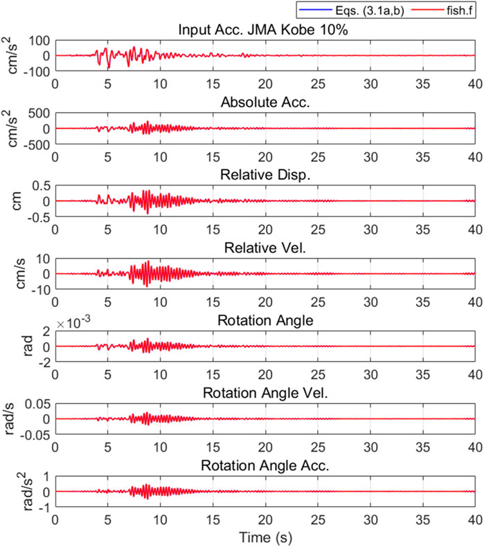
FIGURE 7. Comparison of time history waveforms obtained by our forward fishbone analysis using Eqs 3.1a and 3.1b and time history waveforms obtained by the fish.f analysis for the single-mass system fishbone model.

The system of Eqs 3.2a and 3.2b is rewritten as

$\left[\begin{array}{cc}{h}_1\left({\ddot{x}}_1+\ddot{u}\right)& 0\\ 0& h_1\left({\ddot{x}}_1+\ddot{u}\right)\end{array}\right]\left\{\begin{array}{c}{m}_1\\ m_1\end{array}\right\}=\left[\begin{array}{cccc}2{\theta }_1& 2{\dot{\theta }}_1& \frac{h_1{\theta }_1}{3}& \frac{h_1{\dot{\theta }}_1}{3}\\ 3{\theta }_1& 3{\dot{\theta }}_1& h_1{\theta }_1+x_1& h_1{\dot{\theta }}_1+{\dot{x}}_1\end{array}\right]\left\{\begin{array}{c}{k}_{B1}\\ c_{B1}\\ e_1\\ c_{e1}\end{array}\right\}$(3.3)

When the number of response data for the time history response analysis is $n_d$, Eq. 3.3 can be expressed by

${\mathbf{R}}_{\mathbf{4}}\left\{\begin{array}{c}{m}_1\\ m_1\end{array}\right\}={\mathbf{R}}_{\mathbf{3}}\left\{\begin{array}{c}{k}_{B1}\\ c_{B1}\\ e_1\\ c_{e1}\end{array}\right\},$(3.4)

where

${\mathbf{R}}_{\mathbf{3}}=\left[\begin{array}{cccc}2{\mathbf{\theta }}_{\mathbf{1}}& 2{\dot{\mathbf{\theta }}}_{\mathbf{1}}& \frac{h_1{\mathbf{\theta }}_{\mathbf{1}}}{3}& \frac{h_1{\dot{\mathbf{\theta }}}_{\mathbf{1}}}{3}\\ 3{\mathbf{\theta }}_{\mathbf{1}}& 3{\dot{\mathbf{\theta }}}_{\mathbf{1}}& h_1{\mathbf{\theta }}_{\mathbf{1}}+{\mathbf{x}}_{\mathbf{1}}& h_1{\dot{\mathbf{\theta }}}_{\mathbf{1}}+{\dot{\mathbf{x}}}_{\mathbf{1}}\end{array}\right],$(3.5a)

${\mathbf{R}}_{\mathbf{4}}=\left[\begin{array}{cc}{h}_1\left({\ddot{\mathbf{x}}}_{\mathbf{1}}+\ddot{\mathbf{u}}\right)& 0\\ 0& h_1\left({\ddot{\mathbf{x}}}_{\mathbf{1}}+\ddot{\mathbf{u}}\right)\end{array}\right],$(3.5b)

in which ${\mathbf{\theta }}_{\mathbf{1}}=\left\{\begin{array}{l}{\theta }_{11}\\ {\theta }_{12}\\ ⋮\\ {\theta }_{1n_d}\end{array}\right\},{\dot{\mathbf{\theta }}}_{\mathbf{1}}=\left\{\begin{array}{c}{\dot{\theta }}_{11}\\ {\dot{\theta }}_{12}\\ ⋮\\ {\dot{\theta }}_{1n_d}\end{array}\right\},{\mathbf{x}}_{\mathbf{1}}=\left\{\begin{array}{c}{x}_{11}\\ x_{12}\\ ⋮\\ x_{1n_d}\end{array}\right\},{\dot{\mathbf{x}}}_{\mathbf{1}}=\left\{\begin{array}{c}{\dot{x}}_{11}\\ {\dot{x}}_{12}\\ ⋮\\ {\dot{x}}_{1n_d}\end{array}\right\},{\ddot{\mathbf{x}}}_{\mathbf{1}}+\ddot{\mathbf{u}}=\left\{\begin{array}{c}{\ddot{x}}_{11}+\ddot{u}\\ {\ddot{x}}_{12}+\ddot{u}\\ ⋮\\ {\ddot{x}}_{1n_d}+\ddot{u}\end{array}\right\}$

When the number of steps is $n_d\ne 2$, ${\mathbf{R}}_3$ is not a regular matrix, and the stiffnesses and damping coefficients of beams and columns for the fishbone model of single mass system can be obtained by

$\left\{\begin{array}{c}{k}_{B1}\\ c_{B1}\\ e_1\\ c_{e1}\end{array}\right\}={\left({{\mathbf{R}}_{\mathbf{3}}}^{\mathrm{T}}{\mathbf{R}}_{\mathbf{3}}\right)}^{-1}{{\mathbf{R}}_{\mathbf{3}}}^{\mathrm{T}}{\mathbf{R}}_{\mathbf{4}}\left\{\begin{array}{c}{m}_1\\ m_1\end{array}\right\}.$(3.6)

The evaluated values of $k_{B1}$, $c_{B1}$, $e_1$, $c_{e1}$ from Eq. 3.6 utilizing TDI are exactly equal to the true values of ${\widehat{k}}_{B1}$, ${\widehat{c}}_{B1}$, ${\widehat{e}}_1$, ${\widehat{c}}_{e1}$. When the number of steps is $n_d=1$, the solutions are indeterminate. However, most cases are $n_d>2$.

4 Physical parameter estimation with noise

4.1 Elastic fishbone model of 3-mass system

We investigated the effect of noise on the accuracy of TDI using the elastic fishbone model. We considered the situation where all responses of the 3-mass system fishbone model have random noise. The noise was produced using uniform random numbers, and the maximum range of each response was employed to quantify the noise. Different independent noises were added to the original response data (acceleration, velocity, displacement, rotational angle, and angular velocity) simulated without noise. The data from 5 to 15 s were used for TDI.

Figure 8 plots the percentage errors of the rotational stiffness, rotational damping coefficient, column stiffness, and column damping coefficient with respect to the noise level in the fishbone model of the 3-mass system. It can be observed that the rotational stiffnesses of the first and second stories are evaluated as approximately equal to the true values. The accuracy of the rotational stiffness of the third story and rotational damping coefficients of all stories degrade gradually as noise increases. The order of accuracy degradation in column stiffness and column damping coefficients is larger, and especially the column stiffnesses of the first and second stories and the column damping coefficients of the first story take negative values.

FIGURE 8

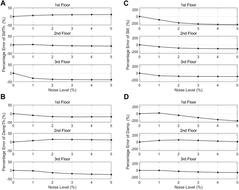
FIGURE 8. Influence of noise level on accuracy of the estimation in the 3-mass system fishbone model: (A) rotational stiffness, (B) rotational damping coefficient, (C) column stiffness, and (D) column damping coefficient.

Figure 9 shows the time history of the moments related to rotational stiffness, rotational damping, column stiffness, and column damping for the first to third rows of Eq. 2.5 as the equation of motion. It can be observed that the moment related to rotational stiffness occupies a large portion of the whole moment, while those related to damping and column stiffness of the first and second stories are small. This shows that the rotational stiffness can be estimated accurately.

FIGURE 9

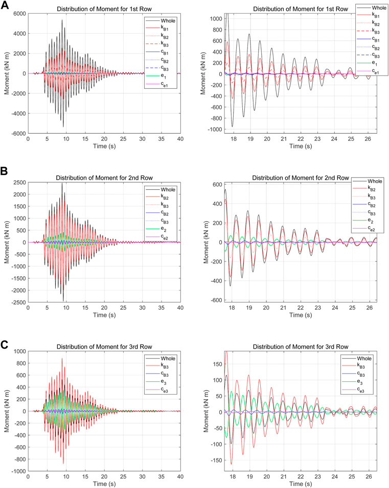
FIGURE 9. Time history of the moments related to rotational stiffness, rotational damping, column stiffness, and column damping for the first to third rows of Eq. 2.5: (A) first row, (B) second row, and (C) third row (left panels: overall view; right panels: enlarged view).

As shown in Figure 9, the moments related to damping are small and they are probably susceptible to noise when solving Eq. 2.5, which is considered to be the reason for the negative damping in Figure 8.

4.2 Elastic fishbone model of single-mass system

We considered the situation in which all responses of the single-mass system fishbone model have noise, similar to the situation described in Section 4.1. It can be observed that the rotational stiffness and rotational damping coefficient are evaluated as approximately equal to the true values, while the accuracies of the column stiffness and column damping coefficient degrade gradually as noise increases.

Figure 10 plots the percentage errors of the rotational stiffness, rotational damping coefficient, column stiffness, and column damping coefficient with respect to the noise level in the fishbone model of the single-mass system. It can be observed that the rotational stiffness and damping coefficient are evaluated as approximately equal to the true values. The accuracy of the column stiffness and damping coefficient degrade gradually as noise increases. Physical parameters of the fishbone model of the single-mass system are estimated more accurately than those of the 3-mass system fishbone model.

FIGURE 10

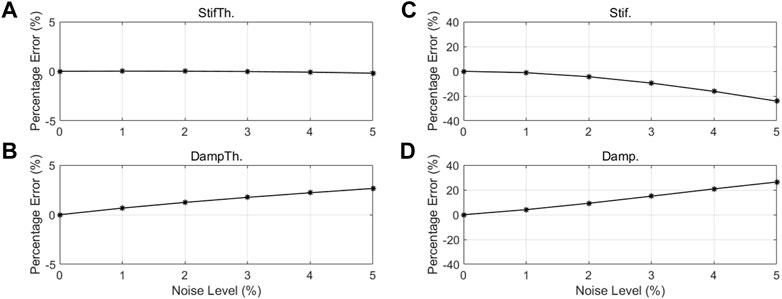
FIGURE 10. Influence of noise level on the accuracy of estimation in the single-mass system fishbone model: (A) rotational stiffness, (B) rotational damping coefficient, (C) column stiffness, and (D) column damping coefficient.

Figure 11 shows the time history of the moments related to the rotational stiffness, rotational damping, column stiffness, and column damping, with Eq. 3.2a as the equation of motion. It can be observed that the moment related to rotational stiffness occupies a large portion of the whole moment, while moments related to the rotational and column damping are small.

FIGURE 11

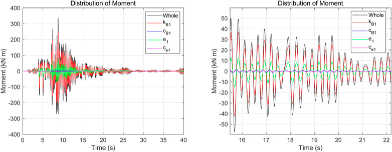
FIGURE 11. Time history of moments related to rotational stiffness, rotational damping, column stiffness, and column damping for Eq. 3.2a (left panel: overall view; right panel: enlarged view).

5 Comparison with mass-spring-dashpot model

TDI was conducted using the mass-spring-dashpot model and the forward analysis results (relative displacement and relative velocity) obtained in Sections 2.3 and 3.2. The shear stiffness and damping coefficient were obtained from the interstory displacement and relative velocity in the inverse analysis using the mass-spring-dashpot model.

5.1 Physical parameter estimation for mass-spring-dashpot model of 3-mass system

TDI was conducted using the mass-spring-dashpot model of a 3-mass system having masses the same as those given in Section 2.3. The evaluated stiffnesses of the springs and damping coefficients of dashpots in each story are shown in Table 8. The ratios of the evaluated stiffness to the column shear stiffness evaluated from the expression $12EI/l^3$ and those of the estimated damping coefficient to the damping coefficient obtained by multiplying $12EI/l^3$ by $2h_c{\omega }_1$ in Eq. 2.4b are shown in Table 9.

TABLE 8

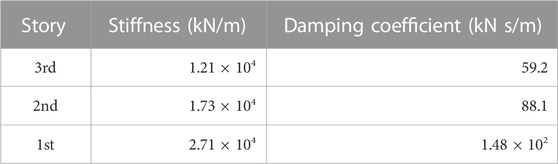
TABLE 8. Evaluated stiffnesses of the springs and damping coefficients of dashpots.

TABLE 9

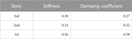
TABLE 9. Ratios of evaluated stiffness to $12EI/l^3$ and estimated damping coefficient to $12EI/l^3$ multiplied by $2h_c{\omega }_1$

Figure 12 compares the time history of waveforms obtained by forward analysis using a mass-spring-dashpot model with the evaluated stiffness of springs and damping coefficient of dashpots and time history waveforms obtained by forward analysis using the fishbone model. There are differences between the results of the shear building model and the results of the fishbone model, especially in the second and third stories.

FIGURE 12

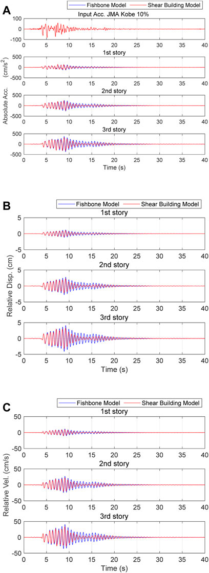
FIGURE 12. Comparison of time history waveforms obtained by forward analysis using the shear building model with the evaluated shear stiffness and damping coefficient and time history waveforms obtained by forward analysis using a fishbone model for the 3-mass system model: (A) absolute acceleration, (B) relative displacement, and (C) relative velocity.

5.2 Physical parameter estimation for mass-spring-dashpot model of single-mass system

TDI was conducted using the mass-spring-dashpot model of a single-mass system having a mass the same as that given in Section 3.2. The evaluated shear stiffness was 2.30 × 10⁴ kN/m. The evaluated damping coefficient was 48.5 kN s/m. The ratio of the evaluated stiffness of spring to the column shear stiffness evaluated from the expression $12EI/l^3$ was 0.56. The ratio of the estimated damping coefficient of dashpot to the damping coefficient obtained by multiplying $12EI/l^3$ by $2h_c{\omega }_1$ in Eq. 2.4b was 0.56.

The estimated damping coefficient of the dashpot was equal to the evaluated stiffness of spring multiplied by $2h_c{\omega }_1$, in the case of the single-mass system, because the damping was assumed to be proportional to the stiffness. $12EI/l^3$ is the shear stiffness when both ends are fixed. When the base is fixed and the other end is free, then the shear stiffness is $3EI/l^3$. The evaluated stiffness value lies between these values because the base is fixed and the other end is supported by the spring in the fishbone model.

Figure 13 compares the time history of waveforms obtained by forward analysis using the shear building model with the evaluated shear stiffness and damping coefficient and time history waveforms obtained by forward analysis using the fishbone model. The result of the shear building model agrees well with the result of the fishbone model for the single-mass system.

FIGURE 13

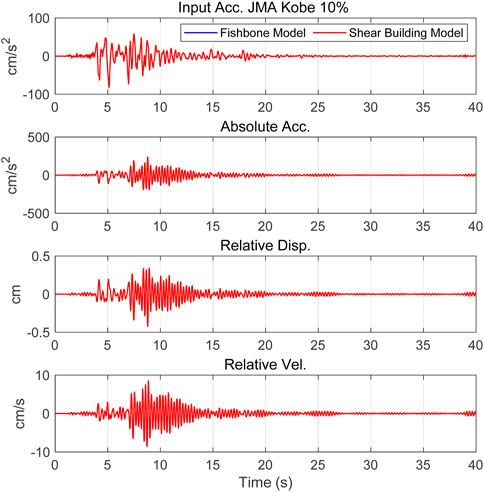
FIGURE 13. Comparison of time history waveforms obtained by forward analysis using the shear building model with the evaluated shear stiffness and damping coefficient and time history waveforms obtained by forward analysis using the fishbone model for the single-mass system model.

6 Conclusion

1) A fishbone model was used to simulate the “Experimental research on seismic safety measures for steel-framed buildings damaged by earthquakes” conducted by E-Defense in 2013. A method of replacing a 3-story steel structure specimen with a fishbone model was developed. Simulations using the obtained fishbone model followed the experimental results well.

2) We formulated the inverse problem for the fishbone model of a multi-mass system. TDI using the forward analysis results without noise in the linear fishbone model of the multi-mass system gave accurate values for the column stiffness, column damping coefficient, beam rotational stiffness, and beam rotational damping coefficient in all 3 stories. When random noise was added to all responses of the forward analysis results, the rotational stiffness and damping coefficient of beams were evaluated almost accurately, but when the noise level increased, the differences between the evaluated values and the real values increased. The stiffness and damping coefficient of columns were not estimated accurately, and, in particular, some of them took negative values.

3) We formulated the inverse problem for the fishbone model of the single-mass system. In the case of a 1-mass model, it is necessary to combine the equation regarding the load and the rotational angle, and the equation regarding the load, the rotational angle, and the relative displacement. TDI using the forward analysis result without noise in the linear fishbone model of the single-mass system gave accurate values for the column stiffness, column damping coefficient, beam rotational stiffness, and beam rotational damping coefficient. When random noise was added to all responses of the forward analysis result, the rotational stiffness and damping coefficient of the beam were evaluated accurately. However, the column stiffness and damping coefficient deviated more from the true values as the noise level increased.

4) TDI was conducted for a mass-spring-dashpot model using forward analysis results for relative displacement, relative velocity, and absolute acceleration for the fishbone model. For the 3-mass system, using the column stiffness and column damping of each story obtained from the inversion analysis of the mass-spring-dashpot model, the time history waveforms of the forward analysis results with the mass-spring-dashpot model were attenuated more than those of the forward analysis result with the fishbone model. For the single-mass system, the results from using the column stiffness and column damping coefficient obtained from the inversion analysis of the mass-spring-dashpot model and the time history waveforms of the forward analysis with the mass-spring-dashpot model almost matched those of the forward analysis results with the fishbone model.

Data availability statement

The original contributions presented in the study are included in the article/Supplementary Material, further inquiries can be directed to the corresponding author.

Author contributions

KK contributed to conception, and all authors contributed to design of the study. AK performed the numerical analysis. RE wrote the first draft of the manuscript. AK and JF wrote sections of the manuscript. All authors contributed to the article and approved the submitted version.

Funding

This work was supported by JSPS KAKENHI Grant Number JP21H01484.

Conflict of interest

The authors declare that the research was conducted in the absence of any commercial or financial relationships that could be construed as a potential conflict of interest.

Publisher’s note

All claims expressed in this article are solely those of the authors and do not necessarily represent those of their affiliated organizations, or those of the publisher, the editors and the reviewers. Any product that may be evaluated in this article, or claim that may be made by its manufacturer, is not guaranteed or endorsed by the publisher.

Supplementary material

The Supplementary Material for this article can be found online at: https://www.frontiersin.org/articles/10.3389/fbuil.2023.1201048/full#supplementary-material

References

Agbabian, M. S., Masri, S. F., Miller, R. K., and Caughey, T. K. (1991). System identification approach to detection of structural changes. J. Eng. Mech. 117 (2), 370–390. doi:10.1061/(asce)0733-9399(1991)117:2(370)

CrossRef Full Text | Google Scholar

Asebi, N. I. E. D. (2023). Experimental research for safety measure of seismic resistance utilizing steel-structure suffered earthquake damage. Appl. Sci., E201303. (accessed 2023-06-15). doi:10.17598/nied.0020

CrossRef Full Text | Google Scholar

Astroza, Rodrigo, Gutiérrez, Gonzalo, Repenning, Christian, and Hernández, Francisco (2018). Time-variant modal parameters and response behavior of a base-isolated building tested on a shake table. Earthq. Spectra 34 (1), 121–143. doi:10.1193/032817EQS054M

CrossRef Full Text | Google Scholar

Balsamo, Luciana, and Betti, Raimondo (2015). Data-based structural health monitoring using small training data sets. Struct. Control Health Monit. 22 (10), 1240–1264. doi:10.1002/stc.1744

CrossRef Full Text | Google Scholar

Brownjohn, James (2007). Structural health monitoring of civil infrastructure. Philosophical Trans. R. Soc. A Math. Phys. Eng. Sci. 365 (1851), 589–622. doi:10.1098/rsta.2006.1925

PubMed Abstract | CrossRef Full Text | Google Scholar

Chang, Peter C., Flatau, Alison, and Liu, S. C. (2003). Review paper: Health monitoring of civil infrastructure. Struct. Health Monit. 2 (3), 257–267. doi:10.1177/1475921703036169

CrossRef Full Text | Google Scholar

Doebling, S. W., Farrar, C. R., Prime, M. B., and Shevitz, D. W. (1996). Damage identification and health monitoring of structural and mechanical systems from changes in their vibration characteristics: A literature review. Los Alamos, NM: OSTI. doi:10.2172/249299

CrossRef Full Text | Google Scholar

Enokida, Ryuta, and Kajiwara, Koichi (2020). Simple piecewise linearisation in time series for time-domain inversion to estimate physical parameters of nonlinear structures. Struct. Control Health Monit. 27 (10), 1–23. doi:10.1002/stc.2606

CrossRef Full Text | Google Scholar

Farrar, Charles R., and Keith, Worden. (2006). An introduction to structural health monitoring. Philosophical Trans. R. Soc. Ser. A Math. Phys. Eng. Sci. 365 (1851), 303–315. doi:10.1098/rsta.2006.1928

PubMed Abstract | CrossRef Full Text | Google Scholar

Fujino, Yozo, Siringoringo, Dionysius M., Ikeda, Yoshiki, Nagayama, Tomonori, and Mizutani, Tsukasa (2019). Research and implementations of structural monitoring for bridges and buildings in Japan. Engineering 5 (6), 1093–1119. doi:10.1016/j.eng.2019.09.006

CrossRef Full Text | Google Scholar

Fujiwara, Jun, Kishida, Akiko, Aoki, Takashi, Enokida, Ryuta, and Kajiwara, Koichi (2021). Changes in the dynamic characteristics of a small-scale gymnasium model due to simulated earthquake damage. J. Disaster Res. 16 (7), 1074–1085. doi:10.20965/jdr.2021.p1074

CrossRef Full Text | Google Scholar

Hearn, George, and Rene, B. Testa (1991). Modal analysis for damage detection in structures. J. Struct. Eng. 117 (10), 3042–3063. doi:10.1061/(asce)0733-9445(1991)117:10(3042)

CrossRef Full Text | Google Scholar

Hyogo Prefecture (2014). Experimental research for safety measure of seismic resistance utilizing steel-structure suffered earthquake damage. Experimental Research Report in March 2014 Available at: https://web.pref.hyogo.lg.jp/kk41/e-defenseh25.html (accessed March 01, 2023).

Google Scholar

Iiyama, Kahori, Kurita, Satoshi, Motosaka, Masato, Chiba, Kazuki, Hiramatsu, Hiroki, and Mitsuji, Kazuya (2015). Modal identification of a heavily damaged nine-story steel-reinforced concrete building by ambient vibration measurements. J. JAEE 15 (3), 3_78–3_94. doi:10.5610/jaee.15.3_78

CrossRef Full Text | Google Scholar

Ji, Xiaodong, Fenves, Gregory L., Kajiwara, Kouichi, and Nakashima, Masayoshi (2011). Seismic damage detection of a full-scale shaking table test structure. J. Struct. Eng. 137 (1), 14–21. doi:10.1061/(asce)st.1943-541x.0000278

CrossRef Full Text | Google Scholar

Kang, Joo Sung, Park, Seung Keun, Shin, Soobong, and Lee, Hae Sung (2005). Structural system identification in time domain using measured acceleration. J. Sound Vib. 288 (1–2), 215–234. doi:10.1016/j.jsv.2005.01.041

CrossRef Full Text | Google Scholar

Kuleli, Muge, and Nagayama, Tomonori (2019). A robust structural parameter estimation method using seismic response measurements. Struct. Control Health Monit. 27, 1–23. doi:10.1002/stc.2475

CrossRef Full Text | Google Scholar

Li, X. Y., and Law, S. S. (2009). Identification of structural damping in time domain. J. Sound Vib. 328 (1–2), 71–84. doi:10.1016/j.jsv.2009.07.033

CrossRef Full Text | Google Scholar

Lynch, Jerome Peter (2007). An overview of wireless structural health monitoring for civil structures. Philosophical Trans. R. Soc. A Math. Phys. Eng. Sci. 365 (1851), 345–372. doi:10.1098/rsta.2006.1932

PubMed Abstract | CrossRef Full Text | Google Scholar

Masri, S. F., Miller, R. K., Saud, A. F., and Caughey, T. K. (1987b). Identification of nonlinear vibrating structures: Part II—applications. J. Appl. Mech. 54 (4), 923–929. doi:10.1115/1.3173140

CrossRef Full Text | Google Scholar

Masri, S. F., Miller, R. K., Saud, A. F., and Caughey, T. K. (1987a). “Identification of nonlinear vibrating structures: Part I—formulation. J. Appl. Mech. 54 (4), 918–922. doi:10.1115/1.3173139

CrossRef Full Text | Google Scholar

Mizushima, Yasunori, Mukai, Yoichi, Hisashi, N. A. M. B. A., Kenzo, T. A. G. A., and Tomoharu, S. A. R. U. W. A. T. A. R. I. (2018). Super-detailed FEM simulations for full-scale steel structure with fatal rupture at joints between members—shaking-table test of full-scale steel frame structure to estimate influence of cumulative damage by multiple strong motion: Part 1. Trans. AIJ 1 (1), 96–108. doi:10.1002/2475-8876.10016

CrossRef Full Text | Google Scholar

Moaveni, Babak, and Asgarieh, Eliyar (2012). Deterministic-stochastic subspace identification method for identification of nonlinear structures as time-varying linear systems. Mech. Syst. Signal Process. 31, 40–55. doi:10.1016/j.ymssp.2012.03.004

CrossRef Full Text | Google Scholar

Nagarajaiah, Satish, and Yang, Yongchao (2017). Modeling and harnessing sparse and low-rank data structure: A new paradigm for structural dynamics, identification, damage detection, and health monitoring. Struct. Control Health Monit. 24 (1), e1851. doi:10.1002/stc.1851

CrossRef Full Text | Google Scholar

Nakamura, Mitsuru, and Yuzuru, Y. A. S. U. I. (1999). Damage evaluation of a steel structure subjected to strong earthquake motion based on ambient vibration measurements. J. Struct. Constr. Eng. Trans. AIJ) 64 (517), 61–68. doi:10.3130/aijs.64.61_1

CrossRef Full Text | Google Scholar

Nakashima, Masayoshi, Ogawa, Koji, and Inoue, Kazuo (2002). Generic frame model for simulation of earthquake responses of steel moment frames. Earthq. Eng. Struct. Dyn. 31 (3), 671–692. doi:10.1002/eqe.148

CrossRef Full Text | Google Scholar

Ogawa, Koji, Hisaya, K. A. M. U. R. A., and Kazuo, I. N. O. U. E. (1999). Modeling of the moment resistant frame to fishbone-shaped frame for the response analysis. J. Struct. Constr. Eng. Trans. AIJ) 64 (521), 119–126. doi:10.3130/aijs.64.119_3

CrossRef Full Text | Google Scholar

Ogawa, Koji (2015). User manual of fish.f Ver.2.3: Response analysis program for fishbone-shaped frame. Hoskote, Karnataka: ADOS, Ltd.

Google Scholar

Shintani, Kenichirou, Yoshitomi, Shinta, and Takewaki, Izuru (2017). Direct linear system identification method for multistory three-dimensional building structure with general eccentricity. Front. Built Environ. 3, 1–8. March. doi:10.3389/fbuil.2017.00017

CrossRef Full Text | Google Scholar

Shintani, Kenichirou, Yoshitomi, Shinta, and Takewaki, Izuru (2020). Model-free identification of hysteretic restoring-force characteristic of multi-plane and multi-story frame model with in-plane flexible floor. Front. Built Environ. 6, 1–16. April. doi:10.3389/fbuil.2020.00048

CrossRef Full Text | Google Scholar

Sohn, Hoon, Farrar, Charles R., Hemez, Francois, and Czarnecki, Jerry (2001). “A review of structural health monitoring literature,” in A Review of Structural Health Review of Structural Health Monitoring Literature 1996-2001, Como, Italy, April 7-12, 2002, 1–7.

Google Scholar

Soma, Kohei, Kanazawa, Kenji, Hara, Kenji, and Haruyuki, K. I. T. A. M. U. R. A. (2016). System identification of a FISH-bone model for using damage detection of steel moment frame building. J. Struct. Constr. Eng. Trans. AIJ) 81 (729), 1831–1841. doi:10.3130/aijs.81.1831

CrossRef Full Text | Google Scholar

Tobita, J. (1996). Evaluation of nonstationary damping characteristics of structures under earthquake excitations. J. Wind Eng. Industrial Aerodynamics 59 (2–3), 283–298. doi:10.1016/0167-6105(96)00012-8

CrossRef Full Text | Google Scholar

Toussi, Sassan, and Yao, James T. P. (1983). Hysteresis identification of existing structures. J. Eng. Mech. 109 (5), 1189–1202. doi:10.1061/(asce)0733-9399(1983)109:5(1189)

CrossRef Full Text | Google Scholar

Xie, L., Mita, A., Luo, L., and MariaFeng, Q. (2018). Innovative substructure approach to estimating structural parameters of shear structures. Struct. Control Health Monit. 25 (4), e2139. doi:10.1002/stc.2139

CrossRef Full Text | Google Scholar