Suspended sediment transport in Rio Colorado agricultural basin, Argentina

The nutrient input from inland water discharges is vital for the development of marine aquatic fauna, being significantly sensitive to changes in water quality (WQ). The assessment of the contribution and distribution of some water quality parameters (e.g., nutrients, metals and inland organic compounds) is of vital importance, especially in irrigation basins. The study area is the Bonaerense Valley of the Colorado River (BVCR) and Mar Argentino, near the mouth of the Colorado River (Buenos Aires, Argentina). The study of water quality parameters is performed in an indirect way, by studying the spatiotemporal dynamics of cohesive sediment (CS), this is possible because the CS has a fundamental role in the transport of substances by adsorption/desorption interactions. We used numerical models (MOHID Land and MOHID Water) in a coupled way, evaluating the complex dynamics involved. The evaluated parameters (flow, velocity, cohesive sediment, salinity and temperature) were calibrated and subsequently validated with data from 7 monitoring stations, located along the Colorado River and adjacent water collectors. Calibration and validation values are within an acceptable range for the purposes, with mean values of 0.8 for NSE (Nash-Sutcliffe model efficiency coefficient), 0.9 (Pearson correlation) for calibration and 0.6 (NSE), 0.9 (Pearson) for validation. The irrigation zone (through the collectors) shows a significative contribution of cohesive sediment, on the order of 300 ppm. The river presents approximately 100 ppm and generates a plume along the coast to the northwest.

1 Introduction

Regarding sediments suspended on water column, we can describe cohesive sediments (CS), which are composed mainly of particles of size <75 μm (silt and clay) and the main property is their cohesive nature, where the forces of attraction predominate over the forces of repulsion, being allegedly a consequence of the amount of clay (greater than 10%). The CS are in interaction with particulate organic matter and with various compounds, which have a wide spectrum of environmental impacts (metals, pesticides, nutrients, and others), therefore, knowing the dynamics of the CS, it is possible to infer approximately and indirectly the dynamics of pollutants and nutrients. (BARROS, 1996) (PORTELA et al., 1997) (VAZ et al., 2011). The dynamics of CS shows a complex phenomena, such as, accumulation by sedimentation and consolidation, and resuspension by erosion, among others (HAYTER and MEHTA, 1986). The drainage network plays a fundamental role in the transport of CS, carrying it from agricultural watersheds to streams, being one of the main responsible for the alteration of water quality, especially in flash floods (VAN RIJN, 2012; BAILLY et al., 2010).

For the study of sediment dynamics in aquatic systems, the numerical models can be used like a powerful tool, where the model is an idealized and simplistic representation of the system. These models fit by applying mathematical equations/functions, therefore if the main physical, chemical and biological processes of the transport are known, the simulation of the current or future conditions of the pollutants are possible. MOHID (Hydrodynamic Model) is the model elected for this work, this model is a three-dimensional water modelling system, developed by MARETEC (Research Center for Marine and Environmental Technology) at the Superior Technical Institute (IST) which belongs to the University of Lisbon in Portugal (Peran et al., 2013). MOHID consists of 2 different models with different integrated modules. In our case the models are used in a coupled way, one of them is MOHID Land, which is based on the resolution of a hydrological transport model designed to simulate the flow of water in a drainage basin and an aquifer (MARETEC.ORG, 2015b), the other model is MOHID Water, a model which simulates the flow and properties of water in surface water bodies (e.g., oceans, estuaries, reservoirs) and solves the shallow water equations using the Finite Volumes method (PERAN, CAMPUZANO, SENABRE, MATEUS, GUTIéRREZ, BELMONTE, ALIAGA, AND NEVES), resolving all the hydraulic characteristics of the body of water studied (LEITAO et al., 2008b).

The study site is situated on the mouth of Colorado River into the Argentine Sea. In that area there are no studies of the dynamics of CS, since there are studies are focused on the river at a considerable distance (about 700 km) over the Andes Mountains, upstream of a dam (COMITE INTERJURIDICCIONAL DEL RIO COLORADO COIRCO, 2020), (BLASI and MANASSERO, 1990), (SPALETTI and ISLA, 2003), According to the aforementioned, this study is novel.

In addition, Argentina has a vast maritime resource, due to the long continental extension of the shelf and a coastline over the Atlantic Ocean, which concentrate an important biodiversity with, in some cases, a significant commercial value (they make up 4% of the country’s exports) (BOSCHI, 1997) (CERVELLINI and PIERINI, 2021), due to this it becomes a potential target of anthropogenic alterations contributed by rivers (PORTELA and NEVES, 1994). The objective of this work is to define the dynamics of cohesive sediments, being the first work and starting point for a comprehensive study, which will provide governmental agencies with a tool for decision making. With the use of a model it is possible to define the dynamics in a continuous time series, as opposed to targeted sampling which gives discrete information in a time series. The fact that the regulated study area is an irrigated area makes it essential to know the water quality along the irrigation canals, and to project a future assessment taking into account the impact on the crops in the area and their subsequent discharge to the ocean.

2 Methods

2.1 Study area

The study area is located in the BVCR, and its coast over the Argentine sea, located in the lower valley of the Colorado River (Buenos Aires, Argentina) on the southern ends of the Villarino district and north of Patagones district of the province of Buenos Aires (39°45.534′S–62°14.781′ W, DMM; Figures 1, 2). The Valley has an irrigated area supplied by waters of the Colorado River and managed by the Development Corporation of the Colorado River (CORFO spanish acronyms), this channel network allows the irrigation of 1,400 km² in a systematized way, on a total of 5,000 km² that includes the Valley. The economic activity in the BVCR is cantered in the horticultural production, although it possesses livestock activity with dairy farms and feedlots (MARINISSEN and ORIONTE, 2015), In this area, the inland waters are discharged into the Argentine sea through irrigation collectors and the mouth of the river itself.

FIGURE 1

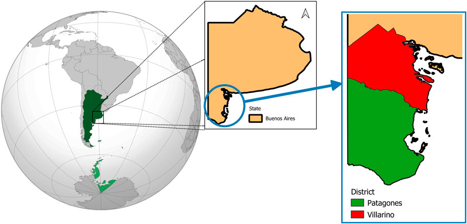
FIGURE 1. Study area.

FIGURE 2

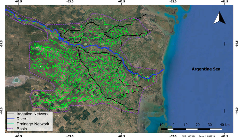
FIGURE 2. Drainage network.

This area is placed at the end of the “Diagonal Árida Sudamericana (South American Arid Diagonal)” stretching from Ecuador to the Atlantic coast of Patagonia, in the Pampa plain. The climate in the region is semi-arid with a progressive aridity to the south [semi-arid zone, classification made by Köeppen (RODRíGUEZ et al., 2018)], the annual rainfall is usually less than 600 mm, the average wind speed approximately of 15.5 km/h predominating from the W-NW and annual average temperature approximate of 14°C–15°C.The river has, within Buenos Aires province, a length over 160 km and covers a drainage area approximately of 6,000 km², this drainage area is covered mostly by an irrigation area (CORFO, 2009; CORFO, 2012) (Figure 2). Within the area there are a small dairy farms and livestock catchment with an amount from 10 to 12 dairy farms, with an approximate milk production of 300–7,000 L/day and an amount of 36,868 cows head, steers, calves and bulls (OF ECONOMICS-U.N.S, 2018). However, traditionally is an agriculture area with irrigation in different modalities such as gravity irrigation and pressurization. Seeds (alfalfa, carrot, cauliflower, hybrid sunflower seeds, corn and sorghum), cereals, oilseeds, horticultural production are mainly grown, where the onion is the crop that represents the main production of the basin and this being the main economic activity of the area (OLAF, 2014).

2.2 Field data collection

Monthly sample from river and irrigation network were collected as shown in Figure 3. The dataset was grouped into two groups, the first of 164 days (calibration), which included from 20/dec/2018 to 01/jun/2019 and a second section of 153 days (validation), from 02/jun/2019 to 02/nov/2019. The water samples were picked up by CORFO and the Environmental Chemistry Laboratory of the National University of the South (Argentina). In situ parameters as flow data and physicochemical parameters (pH, Temperature, salinity) were determined. Then, samples were referred to the laboratory for soil particle size distribution analysis using a Mastersizer 2000 Laser Particle Size Analyzer (Malvern Instruments Ltd., Malvern, United Kingdom).

FIGURE 3

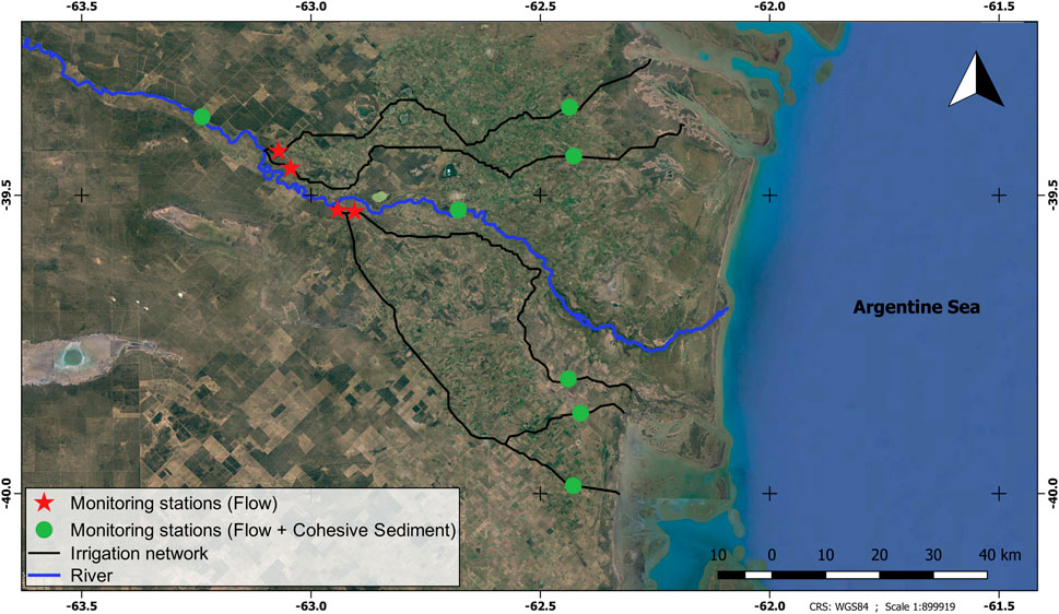
FIGURE 3. Monitoring stations.

2.3 Model description

The models MOHID Land and MOHID Water are in series or coupled, meaning that the output data of MOHID Land are used as input data by MOHID Water. The geographical limits of each model are based on the dominance of the hydrological processes that occur, in the cases where the sea is dominant it uses MOHID Water and the rest of the continental area must be use MOHID Land (Figure 4).

FIGURE 4

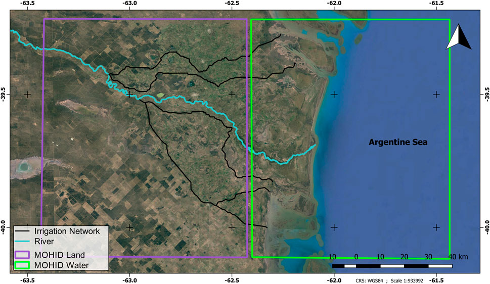
FIGURE 4. MOHID area.

2.3.1 MOHID land

MOHID Land is a model which simulate the water cycle in hydrographic catchments (TRANCOSO et al., 2009). The model considers four compartments or modules (atmosphere, porous media, soil surface, and river network). The atmosphere is not simulated but provides data necessary for imposing surface boundary conditions, the water moves through the remaining mediums based on mass and momentum conservation equations that are computed using a finite volume approach. The simulation domain, just like MOHID Water, is organized into a regular structured grid horizontal plane, and Cartesian type in the vertical plane. (MARETEC.ORG, 2015a). The porous media is a 3D domain which includes the same horizontal grid as the surface (500 × 500 m) with a vertical grid with 5 thickness layers (Table 1), these are based on the Bella Vista series (RODRíGUEZ et al., 2018), with standard hydraulic properties of each horizon. The river network is a 1D domain defined from the digital terrain model (DTM) provided by the National Geographic Institute, with the drainage network linking surface cell centers (nodes) (CANUTO et al., 2019).

TABLE 1

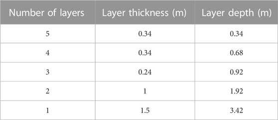
TABLE 1. Vertical layers.

The channel and river cross sections are trapezoidal type with mean dimensions (superficial width, bottom width and height), the dimensions of the drains were trace under Strahler method (Table2). For the fitting of the variables a Manning roughness coefficient of 0.027 is used, this value correspond. s, as explained by CHOW (2004), to an excavated or dredged channel, with short moss/little grass.

TABLE 2

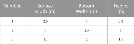
TABLE 2. Strahler dimention values.

In order to define the vegetation type, the report published by INTA (instituto nacional de tecnologia agropecuaria) called the National Crop Map 2018/2019 (INSTITUTO NACIONAL DE TECNOLOGIA AGROPECUARIA, 2019) is considered, dividing the information into 3 groups, grassland (for livestock use), agriculture and without vegetation.

2.3.1.1 Initial and boundary conditions

The atmosphere is provided to impose the conditions of the boudaries of the surface (precipitation, solar radiation, wind, etc.) on the model, the atmospheric parameters (solar radiation, precipitation, etc.) input as time series picked up from Global Forecast System (GFS) data. In the initial conditions for each event analyzed, the surface did not show water columns (dry surface), because of the occurrence of small streams or areas of poor drainage and those where it only flows when it precipitates. This effect was partially compensated applying a correct spin up of the model.

MOHID Water consists of a set of coupled models that aim to simulate the main physical and biogeochemical processes in aquatic systems (MILLER and PINDER, 2004). As MOHID Land, the system is based on the finite volume concept and it is designed in a hierarchical modular structure. The hydrodynamic model (couple model of MOHID Water) solves the momentum and continuity equations for the surface elevation, velocity and flows (MARTINS et al., 2004). Detailed information on the model structure, formulations and default parametrization can be found in https://www.mohid.com/. The bathymetry of the area was obtained by digitizing and interpolating to a Cartesian grid, a nested configuration with three levels of regular spaced grids is implemented, these are called, as shows in Figures 5, 6, Level 1 grid of 1,000 × 1,000 m, Level 2 grids of 200 × 200 m, Level 3 grids of 100 × 100 m (for mouths of each collector of the irrigation network) and Level 3 grids of 50 × 50 m (for river mouth). The approach applied is the downscaling approach, where the large-scale domain and smaller scale domains with better resolution were embedded. The large-scale model runs independently from the smaller-scale model, but these last extracts the necessary information from the larger scale model providing adequate values at its open boundaries and even to the interior of its domain for initial conditions.

FIGURE 5

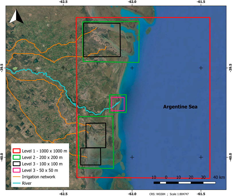
FIGURE 5. Grid area.

FIGURE 6

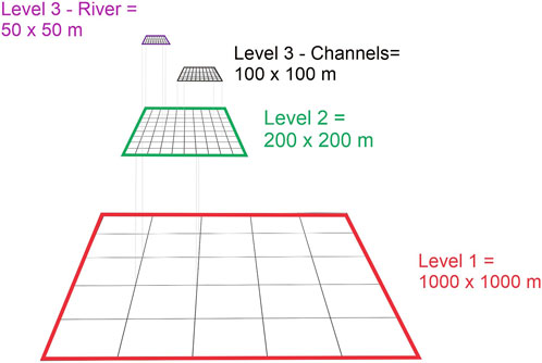
FIGURE 6. Nested grid.

2.3.2.1 Initial and boundary conditions

In this model the boundary conditions can be divided into 3 types: continental, oceans borderline and atmospheric. The first represents the contribution of the streamflow of the river and collectors to the sea, the data are defined as time series output of the MOHID Land model. For oceanic boundary the elevation of the free surface must be specified and in this way the effect of the astronomical tide on the calculation domain is imposed, for that the MOHID tool called MOHID Tide is used, which calculates the elevation of the free surface by superimposing 13 harmonic components of the tide: M2, N2, S2, K2, 2N2, O1, Q1, K1, P1, Mf, Mm, Mtm and MSqm, these components are extracted from the global tidal model FES 2014 (CARRERE et al., 2015). Finally, the atmospheric conditions, as MOHID Land time series input are taken from the GFS.

The initial conditions, applied in the level 1 griddata (1,000 × 1,000 m), are of Dirichlet type, and are imposed by directly specifying the values of the variables at all points of the domain during the initial instant. For the elevation of the free surface a uniform initial value is used (1 m), for the velocity field the initial condition is rest, being necessary a spin up time of.

The initial concentration of CS in the water column is 50 ppm and the concentration of the boundary condition is 22 ppm. For the level 2 and 3 grid data, the type of boundary condition used is open type, where the calculus domain receives information from the near top level.

2.3.2 GFS validation

The initial and boundary atmospheric conditions were provided by the Global Forecast System (GFS) with 0.5° resolution, a model calibration and validation were performed by comparing field measured values of a meteorological station, located in Agricultural Experimental Station INTA - Hilario Ascasubi (39° 37′ S y 62° 37′ O) (Figure 7), this station has measured values of solar radiation, wind, relative humidity and precipitation. For comparison various statistical methods were used, they were divided into three main categories: standard regression statistics (Pearson Correlation Coefficient, Eq. 1), dimensionless (Willmott Concordance Index (WILLMOTT, 1981), Eq. 2) (Nash-Sutcliffe Efficiency Index (NASH and SUTCLIFFE, 1970), Eq. 3); and Uncertainty Index (Standardized Root Mean Square Error (MORIASI et al., 2007), Eq. 4). The results of the methods are shown in Table 3, also in Figure 8 shows a Normalized Taylor diagram to Temperature, Radiation, Precipitation and Relative Humidity (Red: Precipitation; Green: Temperature; Blue: Relative Humidity; Magenta: Radiation). In Figures 9, 10 monitoring station and GFS wind rose during the period 10/2018 to 10/2019 are shown.

$r=\frac{{\sum }_{i=1}^n\left(x_i-\bar{x}\right)-\left(y_i-\bar{y}\right)}{{\sum }_{i=1}^n{\left(x_i-\bar{x}\right)}^2-{\left(y_i-\bar{y}\right)}^2}(1)$

$d=1-\frac{{\sum }_{i=1}^n{\left(s_i-\bar{o}\right)}^2}{\sqrt{{\sum }_{i=1}^n{\left(\mid s_i-\bar{o}\mid +\mid o_i-\bar{o}\mid \right)}^2}}(2)$

$NSE=1-\frac{{\sum }_{i=1}^n{\left(s_i-\bar{o}\right)}^2}{\sqrt{{\sum }_{i=1}^n{\left(o_i-o\right)}^2}}(3)$

$SRMSE=\frac{\sqrt{{\sum }_{i=1}^n{\left(s_i-\bar{o}\right)}^2}}{\sqrt{{\sum }_{i=1}^n{\left(o_i-o\right)}^2}}(4)$

d = Concordance Index.

FIGURE 7

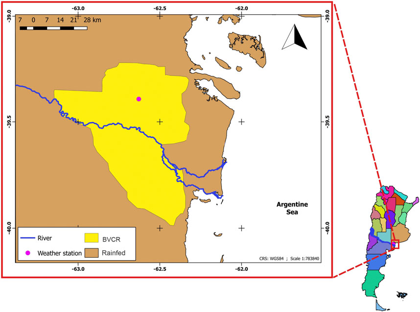
FIGURE 7. Weather station.

TABLE 3

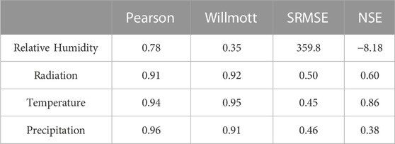
TABLE 3. Statistics indices for comparison.

FIGURE 8

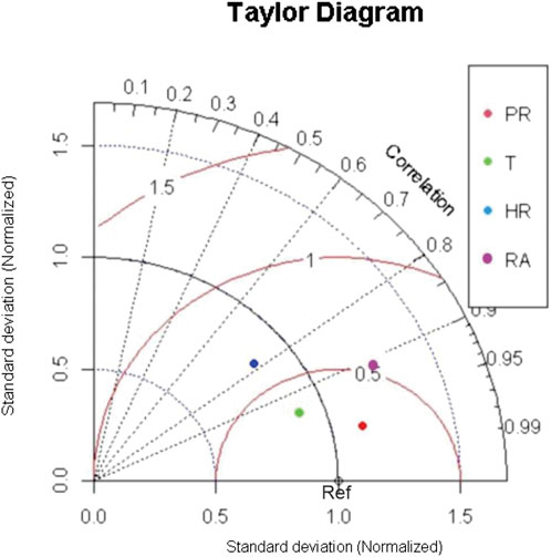
FIGURE 8. Taylor diagram - (T) Temperature (RA) Radiation, (PR)Precipitation, (HR) Relative Humidity.

FIGURE 9

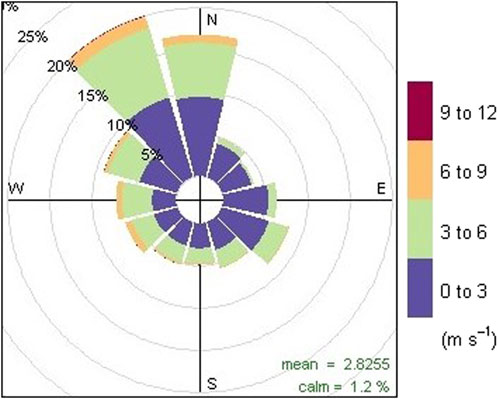
FIGURE 9. Weather station wind rose period 10/2018 to 10/2019.

FIGURE 10

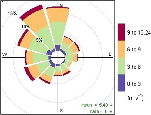
FIGURE 10. GFS wind rose period 10/2018 to 10/2019.

s_i = Simulated values.

o_i = Observed values.

$\bar{o}$ = Average value of n observed values.

NSE = Nash Sutcliffe Efficiency Coefficient.

SRMSE = Standardized Root Mean Square Error.

2.3.3 Cohesive sediment transport

MOHID assumes that the CS transport occurs only in suspension. Thus, the transport depends only on the advection/diffusion equation, with a settling velocity included in the vertical advection (FRANZ et al., 2014). The settling velocity Ws (m.s⁻¹) is considered constant, with a Ws of 5 × 10⁻⁶ m s^-1. The total mass in the model domain can change only due to river inputs and discharges, fluxes across the bottom and fluxes to ocean. The exchange between the water column and the bottom is calculated with the Partheniades erosion formula (Eq. 5) (PARTHENIADES, 1965) and Krone deposition formula (KRONE, 1962) described in Eq. 6:

$\left\{\begin{array}{c}\hfill \frac{\partial M_e}{\partial x}=E\left(\frac{\tau }{{\tau }_E}-1\right)\tau >{\tau }_E\\ \frac{\partial M_e}{\partial x}=0\tau <{\tau }_E\hfill \end{array}\right.(5)$

$\left\{\begin{array}{c}\hfill \frac{\partial M_d}{\partial x}=C{W}_s\left(\frac{\tau }{1-{\tau }_d}\right)\tau <{\tau }_d\\ \frac{\partial M_e}{\partial x}=0\tau >{\tau }_d\hfill \end{array}\right.(6)$

τ = Bed shear stress (Nm^-2). τ_E = Critical shear stress for erosion (Nm^-2). τ_d = Critical shear stress for deposition (Nm^-2).

Consequently, to evaluate the transport of cohesive sediments, the Sediments Module simulates their dynamics in natural systems, taking into account the lower column to represent the bottom stratigraphy, the consolidation of cohesive sediments, the thickness of the sediment column and bathymetry (FRANZ et al., 2017b) (FRANZ et al., 2017a). The fine sediments in the water column are governed by an advection-diffusion equation (LEITAO et al., 2008a), in where the vertical part includes the particle settling velocity and the compute settling are approaches in the Module by 2 different modes: 1- A constant settling velocity, Where the particulate has a specific and constant settling velocity, and 2- A sedimentation velocity dependent on sediment concentration fine, the model uses the algorithm following a formulation described by MEHTA (1988), where the general correlations for the settlement rate in flocculation are extensively described.

2.3.4 Model calibration/validation

As described in section 2.2, the model simulations were conducted between 20/09/2018 and 02/11/2019: the first 3 months (September 20th to 19 December 2018) were used as model “spin-up”; the calibration period was from 20 December 2018 to 1 June 2019 (164 days) and the validation period was from 2 June 2019 to 2 November 2019 (153 days). During the periods described, MOHID Land calibration and validation simulations of hourly streamflow was compared against measured data in the monitoring stations located along the catchment. In this way, the impact on MOHID Land simulations can be assessed. The parameters evaluated were velocity, flow and CS, the statistical indices (minimum, maximum and means) of the model are shown in a Tables 4–6. In order to evaluate the fit of the model MOHID Water, although a global model (FES 2014) calibrated for the tide calculation is used, the Water Level output data of the model is comparing with the tide table of Bahía San Blas (Buenos Aires, Argentina - 40° 34.036′S; 62° 14.411′W), obtaining acceptable statistical indices, Nash-Sutcliffe Efficiency Index (NSE, Eq. 3): 0.32, Pearson Correlation Coefficient (“r”; Eq. 1): 0.99, Standardized root mean square error (SRMSE, Eq. 4): 0.42, percent bias (PBIAS, Eq. 7): 64.94 (GUPTA et al., 1999). The amplitude of the modelled Velocity is compared with that described by the National Meteorological Service (0.25–0.90 m s⁻¹), showing similar values (NATIONAL METEOROLOGICAL SERVICE, 2020). The Validation for MOHID Land was performed by simply comparing model simulations using the parameters in monitoring stations, different goodness of fit tests were considered for assessing model performance, including: “r”, NSE, SRMSE and PBIAS.

TABLE 4

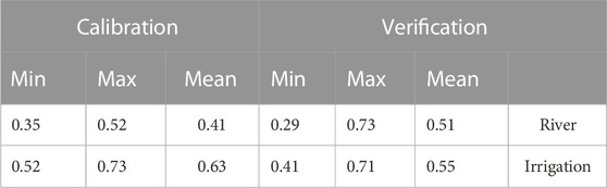
TABLE 4. Velocity (m/s).

TABLE 5

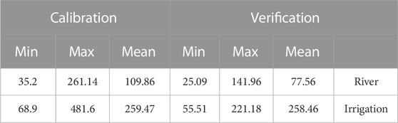
TABLE 5. Cohesive sediment (ppm).

TABLE 6

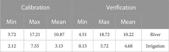
TABLE 6. Flow (m³/s).

Regarding statistical indices, the “r” value close to 1 indicates that the model explains well the variation in observations. When the values of PBIAS (GUPTA et al., 1999) and SRMSE are close to zero, the model predictions are accurate (LEGATES and MCCABE, 1999). The negative or positive sign in PBIAS values indicate the occurrence of under/over estimation bias. Finally, the values close to 1 in NSE (NASH and SUTCLIFFE, 1970) index, refers that the residuals variance is smaller than the observed data variance, hence the model predictions are good. As reference of index values, are used those adjust described byMORIASI et al. (2007) (Table 7)

$PBIAS=100*\left(\frac{{\sum }_{i=1}^n\left(s_i-\bar{o}\right)}{{\sum }_{i=1}^n\left(o_i-o\right)}\right)(7)$

TABLE 7

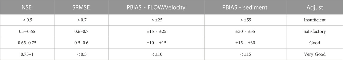
TABLE 7. Statistics indices for adjust.

s_i = Simulated values. o_i = Observed values.

3 Result and discussion

In order to gain a better understanding we analyzed the models MOHID (Land and Water) separately, since only MOHID Land was calibrated and validated (OLIVEIRA et al., 2022) (see subsection 2.3.4), Due to lack of data, the CS concentration and tidal levels for MOHID Water were considered conceptually, this model was previously calibrate and validate in CAMPUZANO et al. (2014).

3.1 MOHID land

3.1.1 Calibration

MOHID Land was run with calibration data, searching for the best possible fit. The results are presented in Table 8 showing the statistical adjustment indices.

TABLE 8

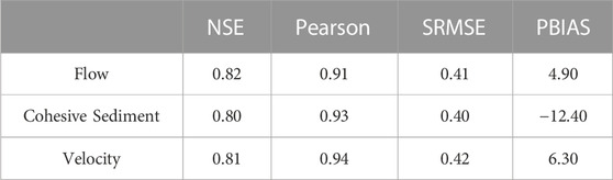
TABLE 8. Statistics indices for comparison.

With the calibration data obtained NSE, SRMSE, PBIAS (Table 7) indices, based on Moriasi work (MORIASI et al., 2007), a very good fit with a strong positive correlation is found.

3.1.2 Validation

Validation was carried out with new data, resulting in the indices shown in Table 9, also correlation between observed data vs. modelled data (calibration and validation stages) (MORIASI et al., 2007) are shows in Figures 11–13.

TABLE 9

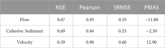
TABLE 9. Statistics indices for comparison.

FIGURE 11

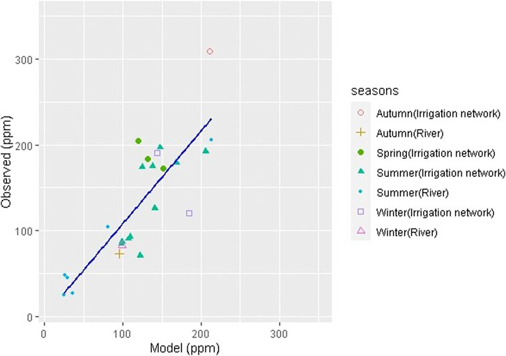
FIGURE 11. Cohesive sediment.

FIGURE 12

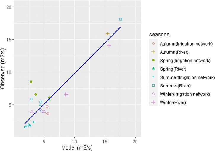
FIGURE 12. Flow.

FIGURE 13

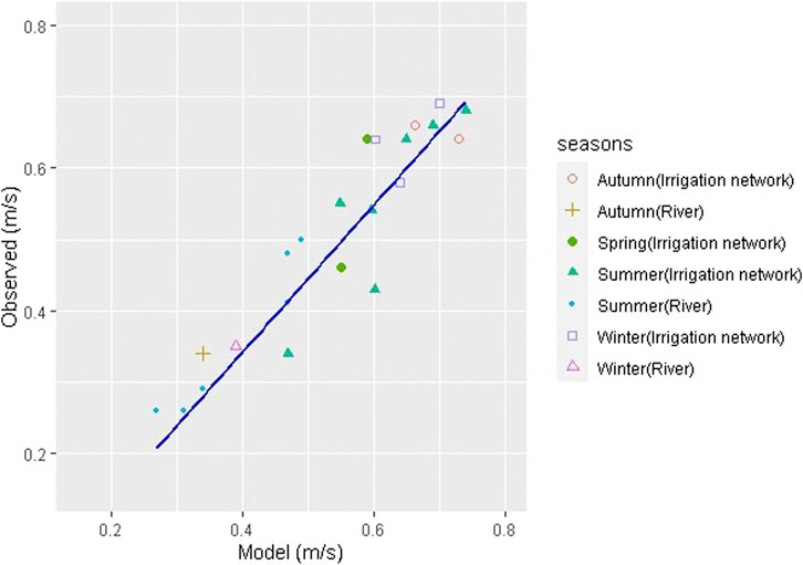
FIGURE 13. Velocity.

The CS and velocity model fit were found acceptable with strong linear correlation, varying in level according to the parameter studied. In terms of flow, the group has a strong linear correlation and a “good” fit (MORIASI et al., 2007) (Table 9). Figures 14–16 show graphs of the variables (velocity, flow and cohesive sediment concentration) as a function of time. They show the drainage network with each irrigation canal and the river. The graphs show the independence of the river flow with respect to the canals, which have a flow controlled by gates. The river flows are maximum between May and September, in apparent agreement with the release of water from the upstream dam. The drainage network has a similar behavior, with higher flows during peak irrigation periods (spring-summer), when it is necessary due to the higher production in the basin (Figure 15). The sediment concentrations of irrigation network are between 80 and 400 ppm throughout the year, showing its independence from rain and runoff (the flow rate does not present significant variations, the high concentration can be due to the work carried out on the channels (Figure 14). In the case of the river, it has concentrations ranging from 18 to 200 ppm, with higher concentrations in summer, coinciding with the time of greater rainfall. In terms of speed, there is a behavior with trends that follow the flow (Figure 16).

FIGURE 14

FIGURE 14. Cohesive Sediment - concentrations (ppm) as a function of time.

FIGURE 15

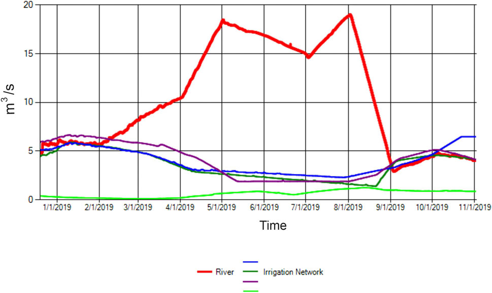
FIGURE 15. Flow (m³/s) as a function of time.

FIGURE 16

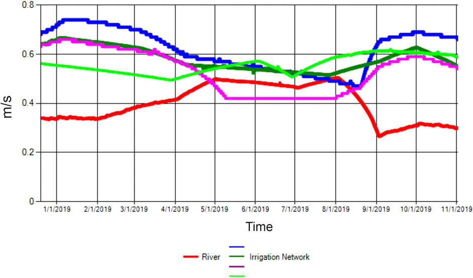
FIGURE 16. Velocity (m/s) as a function of time.

3.2 MOHID water

As a consequence of the pandemic outbreak of SARS-Cov-2, it was not possible to carry out sampling at sea, therefore, the adjustment of the model of CS concentration is considered to be of a conceptual form, leaving open the possibility of being carried out in the future, showing only the dynamic of the CS plume in the sea, modeling the effect of the sea on discharges and their behavior over time. The sediment is distributed along the northern coast, behavior consistent with that found by CAMPUZANO et al. (2014). In that way, it is noted that, except for Collector showed in Figure 17C, the sediment trends to move northwards along the coast, generating deposition and decreasing its concentration. It is also noted the dominance of the tide over the collectors and river, especially in the latter periods of low flow (Figures 17–21), saline intrusion (winter). In the canals, a marked retention of CS is observed over the discharge in the marine channels, being greater in the canal located to the north of the area and the two to the south (19, 20 and 21), this can be attributed to the drainage area they have, since it is greater than the rest. Given the low mixing velocity, it can be assumed that this is an area with a higher concentration of nutrients and marine life, in addition to being an area prone to contaminant transport such as trace metals, organic compounds, bacteria, among others.

FIGURE 17

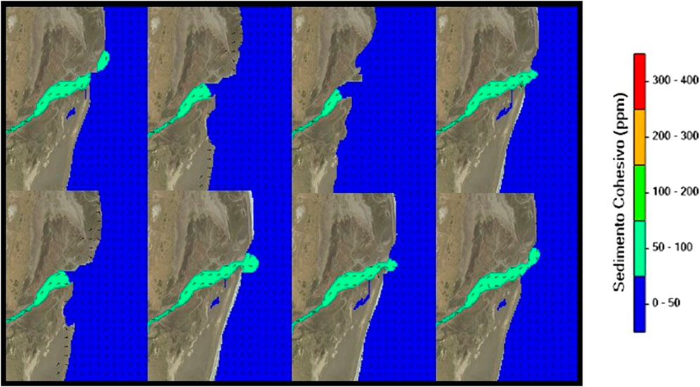
FIGURE 17. CS discharges of river over the sea - 2019/01/03 (00–21 h).

FIGURE 18

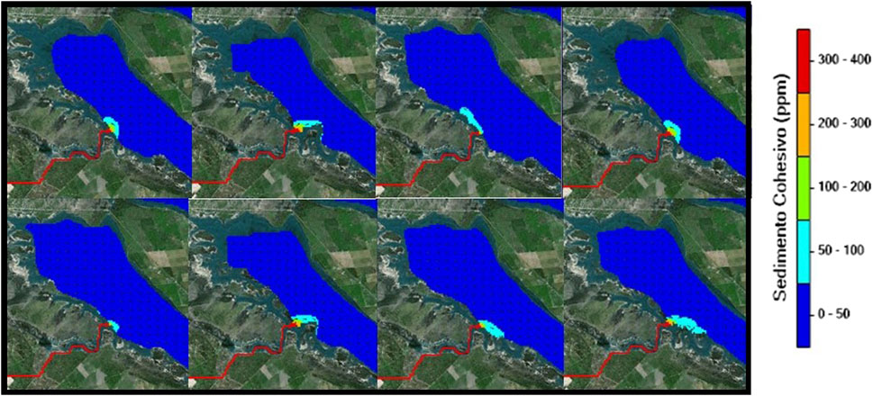
FIGURE 18. CS discharges of Irrigation network over the sea- 2019/01/03 (00–21 h).

FIGURE 19

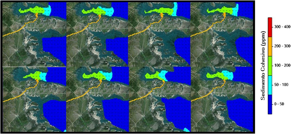
FIGURE 19. CS discharges of Irrigation network over the sea- 2019/01/03 (00–21 h).

FIGURE 20

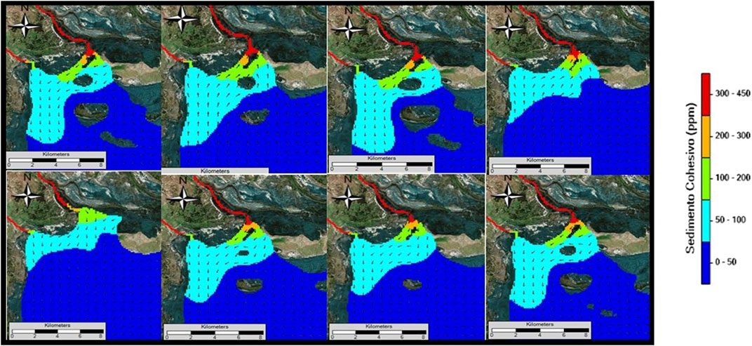
FIGURE 20. CS discharges of Irrigation network over the sea- 2019/01/03 (00–21 h).

FIGURE 21

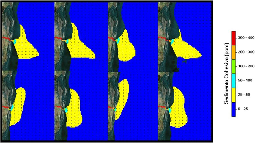
FIGURE 21. CS discharges of Irrigation network over the sea- 2019/01/03 (00–21 h).

4 Conclusion

To conclude, it was possible to calibrate the model correctly, with acceptable statistic index values. MOHID Land was able to integrate the four compartments evaluated (atmosphere, porous media, soil surface, and river network) and simulated successfully the hydrographic basin. In the case of MOHID Water, the water level was calibrated and the velocity was compared semiquantitatively with the interval (mean) values provided by the NATIONAL METEOROLOGICAL SERVICE (2020) of the area of interest (San Blas), being similar to the model value. The coupled model was successfully implemented to simulate (in continent and conceptually in the sea) water flow, velocity and cohesive sediment in the Colorado River basin. It was studied the dynamics of the sediment by defining the direction of plume in the sea during different weather seasons, considering the atmospheric, topographic and tidal influence, having succeeded in implementing for the first time a continental and coastal hydrodynamic simulation study in the Colorado River area. The model could be used for future comparative assessments, both in the management of waste water discharges and in the provision of fresh water from different activities (human, livestock, etc.).This model also generates valuable information that can allow decision-makers to manage and regulate the different activities involved in the basin (tourism sector, crops, irrigation, fishing, etc.) to mitigate impacts on water quality damage. The low exchange rate of marine channels with the sea, observed in some discharges, shows the importance of the study carried out. It can be inferred, for example, that these areas will be rich in nutrients, with the biological importance that this has, generating an opportunity for future studies. Likewise, they will be areas with greater vulnerability to trace metal contaminants, organic and bacterial compounds, among others. The study also shows the areas where there is greater vulnerability to the location of urban waste dumping (areas where there is a CS plume as Conceptual form). Therefore, this work is the starting point for the integral study of resource management in the BVCR basin, generating an opening to diverse fields of study with a direct relevance to the community.

Data availability statement

The original contributions presented in the study are included in the article/Supplementary Material, further inquiries can be directed to the corresponding authors.

Author contributions

NC measured and analyzed the data, JP and NC discussed and wrote sections of the manuscript. JP contributed to review, read, and approve the submitted version.

Funding

This research was funded by the Comisión de Investigaciones Científicas de la Provincia de Buenos Aires (CIC), Ideas Project. Physicochemical and trophic characterization of bonaerense basin of the Colorado River (Act 1480/18). Period: 2019–2020.

Acknowledgments

Contains an acknowledgment of thanks to an agency if this research was funded or supported by that agency, or if there were parties who significantly assisted directly in the research or writing of this article. If the party is already listed as the author, then there is no need to mention it again in this Acknowledgment The authors would like to thank the CORFO, INTA, UNS-INQUISUR and COIRCO institutions for the provided data support. The authors would also like to acknowledge the collaboration with the Instituto Superior Técnico of Lisboa (MARETEC), namely, Ramiro Neves and Francisco Campuzano, and their feedback. Also would like to acknowledge the dedicated efforts of all the staff that is involved in the water sample collection, analysis and data from Environmental Chemistry Laboratory (UNS).

Conflict of interest

The authors declare that the research was conducted in the absence of any commercial or financial relationships that could be construed as a potential conflict of interest.

Publisher’s note

All claims expressed in this article are solely those of the authors and do not necessarily represent those of their affiliated organizations, or those of the publisher, the editors and the reviewers. Any product that may be evaluated in this article, or claim that may be made by its manufacturer, is not guaranteed or endorsed by the publisher.

References

Bailly, D., Brito, D., and Chantha, C. (2010). Assessment of suspended matter transport in a large agricultural catchment using the mohid water modelling system. Strasbourg Cedex, France: European Geosciences Union (EGU), 580.

Google Scholar

Barros, A. (1996). An evaluation of model parameterizations of sediment pathways: A case study for the tejo estuary. Cont. Shelf Res. 16, 1725–1749. doi:10.1016/0278-4343(96)00009-x

CrossRef Full Text | Google Scholar

Blasi, A., and Manassero, M. (1990). The Colorado river of Argentina: Source, climate, and transport as controlling factors on sand composition. J. S. Am. Earth Sci. 3, 65–70. doi:10.1016/0895-9811(90)90018-v

CrossRef Full Text | Google Scholar

Boschi, E. (1997). El mar argentino y sus recursos pesqueros. Instituto nacional de Investigación y desarrollo pesquero, secretaría de Agricultura, ganadería pesca y alimentación, 1, 19.

Google Scholar

Campuzano, F., Pierini, J. O., Leitao, P. C., Gomez, E., and And Neves, R. (2014). Characterisation of the Bahía Blanca estuary by data analysis and numerical modelling. Elsevier Sci. J. Mar. Syst. 129, 415–424. doi:10.1016/j.jmarsys.2013.09.001

CrossRef Full Text | Google Scholar

Canuto, N., Ramos, T., Oliveira, A., Simionesei, L., Basso, M., and And Neves, R. (2019). Influence of reservoir management on guadiana streamflow regime. J. Hydrology Regional Stud. 25, 100628. doi:10.1016/j.ejrh.2019.100628

CrossRef Full Text | Google Scholar

Carrere, L., Lyard, F., Cancet, M., and Guillot, A. (2015). Fes 2014, a new tidal model on the global ocean with enhanced accuracy in shallow seas and in the arctic region egu general assembly conference abstracts. EGU General Assem. Conf. Abstr. 2, 5481.

Google Scholar

Cervellini, P., and Pierini, J. (2021). “Chapter 10: Shrimps and prawns,” in The Bahía blanca estuary. Ecology and biodiversity (Springer).

Google Scholar

Chow, V. (2004). Open-channel hydraulics. Blackburn Press. McGraw-Hill civil engineering series. isbn=9781932846188.

Google Scholar

COMITE INTERJURIDICCIONAL DEL RIO COLORADO (COIRCO) (2020). Programa coirco 1999 a 2020. Available at: https://www.coirco.gov.ar/calidad-del-agua/(Accessed march 2, 2023).

Google Scholar

CORFO (2009). Balance hidrosalino 2006-2009 valle bonaerense del río Colorado. documento corfo (corporación de fomento del valle bonaerense del río Colorado).

Google Scholar

CORFO (2012). Balance hidrosalino 2011-2012 valle bonaerense del río Colorado. documento corfo (corporación de fomento del valle bonaerense del río Colorado). Pedro Luro, Argentina: Science of the Total Environment.

Google Scholar

Franz, G., Delpey, M., Brito, D., LeitãO, P., and Neves, R. (2017). Modelling of sediment transport and morphological evolution under the combined action of waves and currents. Ocean Sci. 13 (5), 673–690. doi:10.5194/os-13-673-2017

CrossRef Full Text | Google Scholar

Franz, G., LeitãO, P., Pinto, L., Jauch, E., Fernandes, L., and And Neves, R. Development and validation of a morphological model for multiple sediment classes. Int. J. Sediment Res. 32(4) (2017), 585–596. doi:10.1016/j.ijsrc.2017.05.002

CrossRef Full Text | Google Scholar

Franz, G., Pinto, L., Ascione, I., Mateus, M., Fernandes, R., LeitãO, P., et al. (2014). Modelling of cohesive sediment dynamics in tidal estuarine systems: Case study of tagus estuary, Portugal. Estuar. Coast. Shelf Sci. 151, 34–44. doi:10.1016/j.ecss.2014.09.017

CrossRef Full Text | Google Scholar

Gupta, H. V., Sorooshian, S., and Yapo, P. O. (1999). Status of automatic calibration for hydrologic models: Comparison with multilevel expert calibration. J. Hydrol. Eng. 4 (2), 135–143. doi:10.1061/(asce)1084-0699(1999)4:2(135)

CrossRef Full Text | Google Scholar

Hayter, E., and Mehta, A. (1986). Modelling cohesive sediment transport in estuarial waters. Appl. Math. Model. 10, 294–303. doi:10.1016/0307-904x(86)90061-2

CrossRef Full Text | Google Scholar

INSTITUTO NACIONAL DE TECNOLOGIA AGROPECUARIA (2019). Mapa nacional de cultivos campaña 2018/2019. Programa nacional de recursos naturales y gestión ambiental.

Google Scholar

Krone, R. Flume studies of the transport of sediment in estuarial shoaling processes. Hydraulic Engineering Laboratory and Sanitary Engineering Research Laboratory. University of California, Berkeley (1962), 110.

Google Scholar

Legates, D., and Mccabe, G. (1999). Evaluating the use of goodness of fit measures in hydrologic and hydroclimatic model validation. Water Resour. Res. 35, 233–241. doi:10.1029/1998wr900018

CrossRef Full Text | Google Scholar

Leitao, P., Mateus, M., Braunchweig, F., Fernandes, L., and And Neves, R. (2008). Modeling coasteal systems: The mohid water numerical lab. Lisbon, Portugal: IST press.

Google Scholar

Leitao, P., Mateus, M., Braunschweig, F., Fernandes, L., and And Neves, R. (2008). “Modelling coastal systems: The mohid water numerical lab,” in Perspectives on integrated coastal zone management in south America. Editors r. Neves, j. Baretta, and m. Mateus (Lisbon: IST Press), 77–88.

Google Scholar

MARETEC.ORG (2015a). Mohid land. Available at: http://wiki. mohid. com/index. php? title= Mohid_Land (Accessed July 21, 2020).

Google Scholar

MARETEC.ORG (2015b). Mohid land/mohid water. Available at: http://www.maretec.org/en/models (Accessed June 26, 2019).

Google Scholar

Marinissen, J., and Orionte, S. (2015). Gestión del recurso humano en el tambo. Buenos Aires, Argentina: INTA Ediciones.

Google Scholar

Martins, F., Leitao, P., Silva, A., and Neves, R. (2004). 3d modelling in the sado estuary using a new generic vertical discretization approach. Oceanol. Acta 24, 51–62. doi:10.1016/s0399-1784(01)00092-5

CrossRef Full Text | Google Scholar

Mehta, A. J. (1988). “Laboratory studies on cohesive sediment deposition and erosion,” in Physical processes in estuaries, job dronkers and wim van Leussen (Springer-Verlag).

CrossRef Full Text | Google Scholar

Miller, C., and Pinder, G. (2004). The object-oriented design of the integrated water modelling system mohid. North Carolina, USA: Elsevier, Chapel Hill, 55.

Google Scholar

Moriasi, D., Arnold, J., VAN Liew, M., and Veith, R. (2007). Model evaluation guidelines for systematic quantification of accuracy in wathersheed simulations. American Society of Agricultural and Biological Engineers, 885–900.

Google Scholar

Nash, J., and Sutcliffe, J. (1970). river flow forecasting through conceptual models: Part 1. A discussion of principles. J. Hydrology 10, 282–290. doi:10.1016/0022-1694(70)90255-6

CrossRef Full Text | Google Scholar

NATIONAL METEOROLOGICAL SERVICE (2020). Numerical models. Available at: https://www.smn.gob.ar/modelos#dropdown4_2-tab (Accessed August 19, 2020).

Google Scholar

Of Economics-U.N.S, D. (2018). “Estimación del producto agropecuario regional,” in Banco de datos Socioeconomicos de la Zona de CORFO -Rio Colorado.

Google Scholar

Olaf, J. (2014). Plan estratégico territorial de la región del rio Colorado. programa de fortalecimiento institucional de la subsecretaría de planificación territorial de la inversión pública. Gorbierno de la Republica Argentina, Buenos Aires, Argentina.

Google Scholar

Oliveira, A., Ramos, T., Simionesei, L., GonçALVES, M., and And Neves, R. (2022). Modeling streamflow at the iberian peninsula scale using mohid-land: Challenges from a coarse scale approach. Water 14, 1013. doi:10.3390/w14071013

CrossRef Full Text | Google Scholar

Partheniades, E. (1965). Erosion and deposition of cohesive soils. J. Hydraulic Eng. 91, 105–139. doi:10.1061/jyceaj.0001165

CrossRef Full Text | Google Scholar

Peran, A., Campuzano, F., Senabre, T., Mateus, M., GutiéRREZ, J., Belmonte, A., et al. (2013). Ocean modelling for coastal management - case studies with mohid, 265.

Google Scholar

Portela, L. (1997). “Effect of settling velocity on the modelling of suspended sediment transport,” in Computer modelling of seas and coastal regions iii. Editors J. R. Acinas, and C. A. brebbia (La Coruna, spain: Computational Mechanics Publications), 347–403.

Google Scholar

Portela, L., and Neves, R. (1994). Numerical modelling of suspended sediment transport in tidal estuaries: A comparison between the tagus (Portugal) and the scheldt (Belgium-the Netherlands). Neth. J. aquatic Ecol. 28, 329–335. doi:10.1007/bf02334201

CrossRef Full Text | Google Scholar

RodríGUEZ, D., Schulz, G., and Morett, L. (2018). Carta de suelos, partido de villarino provincia de buenos aires. argentina: Ediciones INTA.

Google Scholar

Spaletti, L. A., and Isla, F. I. (2003). Caracteristicas y evolucion del delta del rio Colorado "colú-leuvú. Rev. Asoc. Argent. Sedimentol. 10, 23–37.

Google Scholar

Trancoso, A., Braunschweig, F., Chambel LeitãO, P., Obermann, M., and And Neves, R. (2009). An advanced modelling tool for simulating complex river systems. Sci. Total Environ. 407, 3004–3016. doi:10.1016/j.scitotenv.2009.01.015

PubMed Abstract | CrossRef Full Text | Google Scholar

VAN Rijn, L. (2012). Principles of sedimentation and erosion engineering in rivers, estuaries and coastal seas. Netherlands: Aqua Publications, 580.

Google Scholar

Vaz, N., Mateus, M., and Dias, J. (2011). Semidiurnal and spring-neap variations in the tagus estuary: Application of a process-oriented hydro-biogeochemical model. J. costal Res., 1619–1623.

Google Scholar

Willmott, C. I. (1981). On the validation of models. Phys. Geogr. 2, 184–194. doi:10.1080/02723646.1981.10642213

CrossRef Full Text | Google Scholar