Effect of soil anisotropy and variability on the stability of undrained soil slope

Soil is a naturally heterogeneous material and can show significant spatial variation in strength and other properties. For silty and clayey soils, these variations are often more pronounced. Despite such variation, many past studies considered these soils as homogeneous and only considered a single set of soil parameters. This may lead to underestimation of the failure potential of geo-structure such as natural slopes, water retaining dams, retaining walls, etc. A finite element method considering soil variability should be an ideal tool to investigate the behaviour of these soils. This study adopted a 2D random finite element method to evaluate the effect of such variability on slope stability. The spatial variability was implemented by using the coefficient of variation (COV) and the spatial correlation length (θ) for cohesion. It was found that the soil slope with higher COV would have a higher chance of failure, whereas the soil slope with less COV might not show any failure. In addition, the soil with a higher θ, in general, show less potential of failure. In the literature, most studies considered an isotropic condition for the soil, i.e., θ in x and y directions are the same θ_x = θ_y, which is not realistic. Therefore, the soil anisotropy (i.e., θ_x ≠ θ_y) was considered carefully in this study. It was found that the probability of failure for anisotropic soil might be significantly higher than the isotropic soil.

Introduction

Soil slopes, i.e., cuttings or embankments, are an integral part of our transport network. Since the variability of material quality is common in soils, especially for silty or clayey soils (Karim et al., 2011; Devkota et al., 2022; Karim et al., 2022), the uncertainty on the stability of these slopes is an inherent challenge (Griffiths, 1982; Huang et al., 2006; Gould et al., 2011; Kasama and Whittle, 2011; Karim et al., 2021). Further, the mechanics for slope stability analysis that involves the conventional limit state approach uses simplifications and approximations, which adds to the uncertainty of their design. Thus designers often use a highly conservative estimation of strength parameters (Griffiths and Lane, 1999). The assumption of homogenous soil is also common in geotechnical designs, even though the strength parameters may vary spatially (Idriss et al., 1978; Huang et al., 2013; Rahman and Nguyen, 2013). Therefore, an alternative approach that allows natural soil characteristics of spatial variability is needed to quantify the related risk of failure.

In recent years, an advanced numerical technique that uses a combination of the finite element method (FEM) and random field model (RFM) has been gaining popularity and is capable of capturing the soil characteristics of spatial variability in soil properties (Griffiths and Lane, 1999; Griffiths and Fenton, 2001; Fenton and Griffiths, 2003; Fenton and Griffiths, 2008; Rahman and Nguyen, 2012; Huang et al., 2013; Li et al., 2019). Griffiths and Fenton, (2001) adopted a technique called local average subdivision (LAS) for generating a random field for undrained shear strength. This technique was first introduced by Fenton (1990), and then it was revisited by others (Fenton and Vanmarcke, 1990; Fenton and Griffiths, 2007) based on the probability density and spatial correlation functions for soil parameters. The main advantage of this approach is the capability of capturing the complex behaviour of soil with high spatial variability.

In this study, the FEM with a random field generator is used for slope stability analysis. This method is also referred to as the random finite element method (RFEM), as proposed by Griffiths and Fenton, (2001). RFEM has been applied in many different areas of geotechnical engineering, such as bearing capacity under foundation, slope stability, pile foundation, etc. (Smith and Griffiths, 1998; Griffiths and Lane, 1999; Fenton and Griffiths, 2008; Jiang et al., 2022a; Jiang et al., 2022b; Nguyen et al., 2022; Shu et al., 2023). It allows the soil properties to be changed spatially but still correlated with the neighbouring soils (Fenton and Vanmarcke, 1990; Fenton and Griffiths, 2007). Griffiths and Fenton, (2001) proposed correlation length (θ) as a measure for investigating the correlations between neighbouring soils. Based on the correlation length and soil variability, the random field for soil parameters can be generated. One of the most efficient random field generation techniques is the local average subdivision (LAS), which was introduced in Vanmarcke (1984). This technique considers a global average for a parent cell. Then, the cell is subdivided multiple times. The local average in each child cell is recalculated. This technique ensures a reasonable transition in soil parameters between the neighbouring cells. It should be noted that there have been different studies considering other techniques for generating a random field. One notable approach, the numerical limit analysis (Kasama and Whittle, 2011) (NLA) is based on the numerical formulations of upper and lower bound limit analyses for rigid perfectly plastic materials, using finite element discretisation and linear (Sloan, 1988; Sloan and Kleeman, 1995) or non-linear programming methods (Lyamin and Sloan, 2002a; Lyamin and Sloan, 2002b). According to Kasama and Whittle (2011), both upper and lower bound analysis treats the soil elements as three-node triangular elements. By applying the upper and lower bound limits, the calculated failure load was covered into a range. However, the NLA technique may produce results that do not align well with the theoretical data, whereas the LAS technique can produce the best-fit results with the theoretical values. Therefore, this research considered the LAS technique for generating a random field.

Most RFEM studies in slope stability considered an isotropic condition in which the correlations between neighbouring soils in lateral and vertical directions are the same (Griffiths and Fenton, 2004; Griffiths et al., 2015; Kasama and Whittle, 2016; Zhu et al., 2017). However, an anisotropic condition is more common in nature. Soils in their natural states deposit in layers, and their strength and other properties can be different in vertical and lateral directions, i.e., anisotropic conditions prevail. Most previous studies often found the correlation lengths in the horizontal direction were higher than in the vertical direction (DeGroot and Baecher, 1993; Vessia et al., 2009; Rahman and Nguyen, 2013).

There have been some studies that incorporated soil anisotropy (Rahman and Nguyen, 2013; Nguyen and Rahman, 2015; Pieczyńska-Kozłowska et al., 2015; Li et al., 2016; Zaskórski et al., 2017) in bearing capacity problems. Some studies were done for slope stability. Akbas and Huvaj (2015) only evaluated different combinations of correlation length with a single value of the coefficient of variation (COV) of 0.2, which represented slightly varied soil. Liu et al. (2018) investigated the stability of 3D slope with one combination of correlation length (θ_x = 2H and θ_y = 0.4H, where H is the height of the slope) and COV of 0.3 for undrained cohesion. The studies using COV less than 1.0 may not be able to capture the randomness of highly varied materials such as tailings, etc. Other studies (Huang et al., 2013; Li et al., 2019) examined the finite element strength reduction analysis in RFEM; however, the ranges of COV and correlation are not wide enough to explore different possibilities of a factor of safety. Therefore, the combined effect of soil anisotropy and variability on the probability of slope failure is not fully understood, mostly due to a limited number of past studies incorporating anisotropy and limited data sets available. Therefore, this research adopts the RFEM approach from Griffiths’ group (Griffiths and Lane, 1999; Griffiths and Fenton, 2001) with LAS to consider the soil variability, simulates both isotropic and anisotropic conditions by combining a wide range of coefficients of variation (COV) of soil properties and correlation lengths in the vertical and horizontal directions and then investigate the combined effects of correlation length and soil anisotropy on slope stability. This study produces a comprehensive data set of anisotropic conditions for correlation lengths for the main investigation.

A probabilistic method for slope stability

The stability of a soil slope in the undrained condition is often analysed using a set of soil properties/parameters consisting of the undrained shear strength (c_u), the undrained friction angle (ϕ_u), and the saturated unit weight (γ_sat). In the deterministic approach, these parameters are assumed to be constant, i.e., a homogenous soil. The friction angle, ϕ_u, for silty or clayey soils can be taken as zero. For simplicity, γ_sat is also held constant at 20 kN/m³. Other important parameters for the slope are the slope inclination (ß), the height of slope (H) and the depth of foundation indicated by n_d. An illustration of the slope used for analysis is shown in Figure 1. The soil strength parameters are reduced during the analysis to capture the failure of the slope.

FIGURE 1

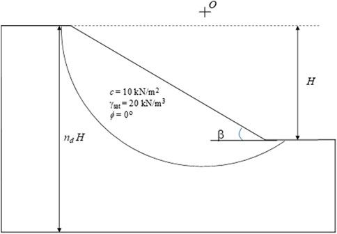
FIGURE 1. An illustration of the slope geometry in this study.

The undrained cohesion (c_u) is allowed to vary spatially, and its effect on slope stability is examined. To compare with the deterministic approach, c_u is generalised and expressed in terms of a dimensionless parameter (C) by normalising against the multiplication of unit weight and slope height.

$C=\frac{c_u}{{\gamma }_{sat}H}(1)$

Two different approaches are adopted to generate the spatial variation of C in the slope geometry, namely, the single random variable approach and the random variable approach considering spatial correlation length. In the single random variable approach, a lognormal distribution function for C was adopted to avoid the unreasonable negative value of C and to ensure positive shear strength by the random field generator. After Griffiths and Fenton (2004), the probability density function of C is expressed as a log-normal distribution function (see Figure 2):

$f\left(C\right)=\frac{1}{C{\sigma }_{\ln C}\sqrt{2\pi }}\exp \left[-0.5{\left(\frac{\ln C-{\mu }_{\ln C}}{{\sigma }_{\ln C}}\right)}^2\right](2)$

where μ_lnC and σ_lnC are the mean and standard deviation of the natural logarithm of C. μ_lnC and σ_lnC are determined by the dimensionless coefficient of variation (COV), which is defined as the ratio μ_C and σ_C as shown below.

$CO{V}_C={\sigma }_C/{\mu }_C(3)$

FIGURE 2

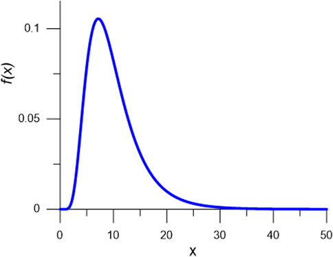
FIGURE 2. Log-normal distribution function for C.

According to Eq. 1, the COV of the dimensionless parameter (C) was equal to COV_cu ($CO{V}_{cu}={\sigma }_{cu}/{\mu }_{cu}$), as γ_sat and H were kept constant in this study. The distribution of ln(C) is then characterised by:

${\sigma }_{\ln C}=\sqrt{\ln \left(1+CO{V_C}^2\right)}(\mathrm{4a})$

${\mu }_{\ln C}=\ln {\mu }_C-0.5{{\sigma }_{\ln C}}^2(\mathrm{4b})$

To continue with the calculation of the probabilistic failure, the chance of failure has to be defined by the probability of random C less than the characteristic value of C. For this, a random value of C from the probability function of Eq. 2 was assigned for the entire slope. Therefore, the slope is still homogeneous. According to Griffiths and Fenton (2004), the relationship between C and the factor of safety (FOS) of the homogeneous slope can be presented in Table 1. The data in Table 1 shows a linear relationship (plotted in Figure 3) between C and FOS with a very high coefficient of determination (R²∼1).

TABLE 1

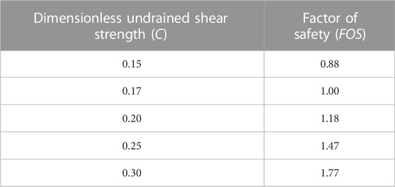
TABLE 1. The factor of safety of a homogeneous slope in a deterministic approach (Griffiths and Fenton, 2004).

FIGURE 3

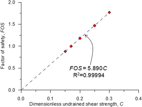
FIGURE 3. The relationship between C and FOS of a homogeneous slope.

Based on the data in Table 1 and Figure 3, the characteristic value of C for a slope with FOS of 1.00 is 0.17. Hence, the chance of failure of the slope in this probabilistic study can be expressed as:

$p_f=p\left[C<0.17\right]=\mathrm{\Phi }\left(\frac{\ln 0.17-{\mu }_{\ln C}}{{\sigma }_{\ln C}}\right)(5)$

In the second analysis with the spatial correlation, one of the important parameters will be the spatial correlation length (θ_lnC) (Griffiths and Fenton, 2001). When C is log-normally distributed, its logarithm yields an underlying Gaussian field. θ_lnC, which is the measure of this Gaussian field, ensures that the neighbouring soils in the slope are still correlated. A normalised dimensionless measure of θ_lnC (Θ_lnC) can be presented by the ratio of θ_lnC and H. The representative value of θ_lnC for clay has not been clearly defined in the literature (Griffiths and Fenton, 2001), especially in the horizontal directions. This is because the soil normally deposits into layers and the higher variation in the vertical direction is more likely to be observed. This analysis is presented in the following section.

It should be noted that the Monte Carlo simulation was adopted in this study. This method uses the estimation of randomly stochastic soil property based on its distribution type, mean and standard deviation. The Monte Carlo simulation also uses the correlation function or spectral density function, which is also a characteristic of spatial variability for cohesion. Each test considered 1,000 Monte Carlo simulations.

Effect of soil variability and anisotropy on slope stability

As mentioned previously, the elastoplastic FEM coupling with the probabilistic approach is an effective tool that can better capture the effect of variability of soil in the slope stability problem (Akbas and Huvaj; Griffiths and Fenton, 2004; Vessia et al., 2009; Huang et al., 2013; Rahman and Nguyen, 2013; 2015; Pieczyńska-Kozłowska et al., 2015). The discretised geometry used in this study is presented in Figure 4 and the LAS technique is adopted for generating the random field due to its efficiency and accuracy. The mean undrained cohesion is chosen as 100kPa, and the standard deviations for the undrained cohesion are 25kPa, 50kPa, 100kPa, 200kPa, 400kPa and 800 kPa respectively.

FIGURE 4

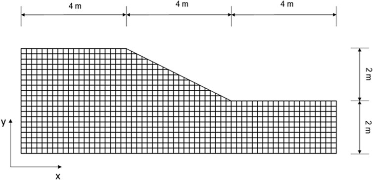
FIGURE 4. The discretised geometry of the slope for RFEM study.

Each mesh in Figure 4 has a corresponding value of C throughout the generating process in the LAS technique. The correlation function between two distant points is defined by the Markovian function (Fenton and Griffiths, 2008) as

$\rho \left(\left|X_{ij}\right|,\left|Y_{ij}\right|\right)=\mathit{exp}\left\{-\surd {\left(2X_{ij}/{\theta }_x\right)}^2+{\left(2Y_{ij}/{\theta }_y\right)}^2\right\}(6)$

where X_ij and Y_ij are the distances between two random points in horizontal and vertical directions respectively. The correlation field of C will be different with different combinations of θ_x andθ_y. Figure 5 demonstrates the capacity of different combinations of θ_x andθ_y to generate the correlation field or correlation coefficient (ρ). Figures 5A–C show the symmetrical distributions of ρ for the isotropic conditions.

• For a lower correlation length (θ_x = θ_y = 1.0), the highest correlation is achieved when the random points are closer to each other i.e., X_ij and Y_ij are nearly zero. When the two random points are far away from each other, ρ reduces significantly.

• For a higher correlation length (θ_x = θ_y = 10 or 100), ρ only reduces slightly, when the two random points are far away from each other.

FIGURE 5

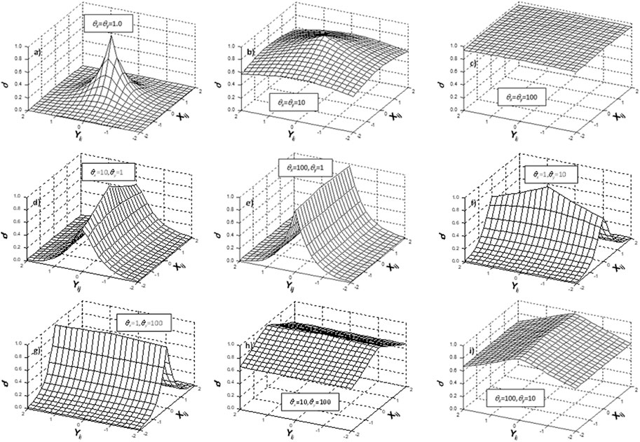
FIGURE 5. The correlation coefficient, pin 2-D: (A) ${\theta }_x={\theta }_y=1$; (B) ${\theta }_x={\theta }_y=10$; (C) ${\theta }_x={\theta }_y=100$; (D) ${\theta }_x=10\&{\theta }_y=1$; (E) ${\theta }_x=100\&{\theta }_y=1$; (F) ${\theta }_x=1\&{\theta }_y=10$; (G) ${\theta }_x=1\&{\theta }_y=100$; (H) ${\theta }_x=10\&{\theta }_y=100$; (I) ${\theta }_x=100\&{\theta }_y=1$ 0.

In Figures 5D–I, the distributions of ρ for the anisotropic conditions are shown. When θ_x >θ_y, 𝜌_y reduces faster than 𝜌_x in the case of two far random points, and vice versa. It should be noted that when θ_x orθ_y is very high and approaching infinity, the correlation coefficient, ρ is approaching 1. This means 100% correlation between two random points, which is an optimistic assumption in the design.

The correlation coefficient (ρ) between separated points in anisotropy was much different with different combinations of the correlation lengths. ρ tends to increase to 1 in the x-direction while θ_x is continuously increasing up to infinity. The random set of variables obtained from the correlation function is later used to transform the random field of c within the random field with available mean and standard deviation. The lognormal transformation is defined as

$c\left(i,j\right)=e^{\mu +\sigma G\left(i,j\right)}(7)$

where G is a standard lognormal variable, which is defined throughout the LAS process. Then the function used to subdivide the mesh in the LAS process is adopted:

$G=A^{T}Q+LU(8)$

where U is indicated as the vector of independent standard normal random variables with mean zero and unit standard deviation. The covariance describing the relationship between the cells can be calculated by the matrix multiplication with a transpose

$R=E\left[Q{Q}^T\right](9)$

$S=E\left[Q{G}^T\right](10)$

$B=E\left[G{G}^T\right](11)$

where R is the covariance between the parent cells, S is the covariance between the parent and child cells and B is the covariance between the child cells. Then the matrices A and L in Eq. 8 can be determined by

$A=R^{-1}S(12)$

$L{L}^T=B-S^{T}A(13)$

The study considers a wide range of θ_x,θ_y and COV to investigate the combined effect of correlation length and COV on the probability of failure.

• Six of values of θ_x: 0.2, 0.5, 1.0, 2.0, 4.0 and 8.0 m

• Six of values of θ_y: 0.2, 0.5, 1.0, 2.0, 4.0 and 8.0 m

• Six of values of COV: 0.25, 0.5, 1.0, 2.0, 4.0 and 8.0

One combination of θ_x,θ_y and COV gives one p_f. In total, there are 216 simulations in this study. The details can be found in Table 2.

TABLE 2

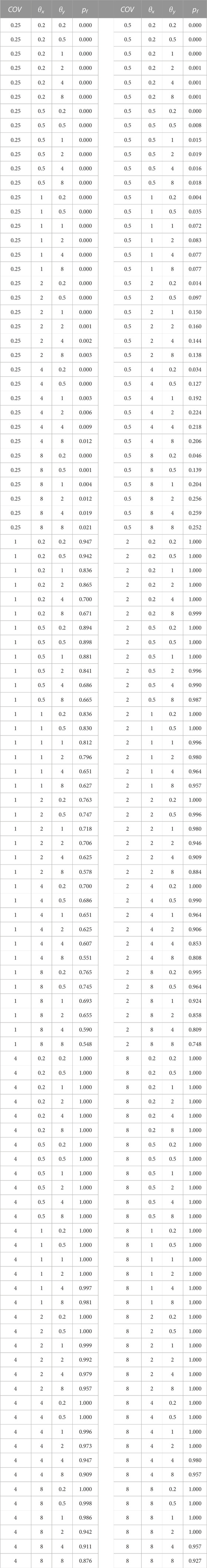
TABLE 2. The details of RFEM simulations used in this study.

The slope with a small variation of soil parameters (i.e., low COV of 0.25–0.50 and high θ of 8 m), a smooth random field can be observed (see Figure 6). Figure 6A shows the variation of c_u and the deformations of the cells; whereas Figure 6B shows only displacement vectors. It should be noted the darker colour in Figure 6A means a higher value for cohesion. There is no failure surface appearing in this case, as the displacement vectors do not reach the right side of the slope in Figure 6B. As mentioned before, the elements were assigned different C parameters. The failure mechanism will pass through these elements by find the weakest zone based on the assigned parameters. The slope will fail if the deformation or displacement is significant. It noted that this research also considered the shear strength reduction technique for the slope stability analysis (Griffiths and Lane, 1999).

FIGURE 6

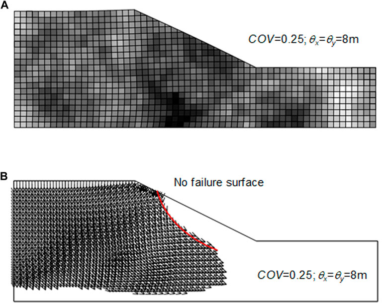
FIGURE 6. Slope stability for soils with slight variation (COV = 0.25, ${\theta }_x={\theta }_y=8m$). (A) deformed meshes and (B) displacement vectors’.

On the other hand, if the soils have high variation (i.e., high COV) and small correlation (i.e., small θ), the cohesion field is ragged. In this case, cohesion values of neighbouring soils are mostly random at the final state of the slope analysis as shown in Figure 7A, and the probability of failure is 100%. The failure line appears on the slope and follows the weakest path traversing the weakest points in the slope geometry. The directions of the displacement vectors also follow the same weakest path as shown in Figure 7.

FIGURE 7

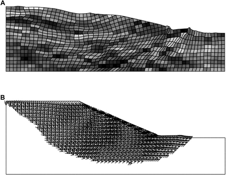
FIGURE 7. Slope stability for soils with high variation (COV = 4.0, ${\theta }_x={\theta }_y=0.2m$). (A) deformed meshes and (B) displacement vectors’.

The traditional approach for slope stability analysis often assumes a deterministic value for soil strength as mentioned previously. This means that the soil parameters have no variation, which is similar to the case presented in Figure 6. In such a case, the chance of failure is very low. However, the assumption of slight variation for a parameter is not always true for most soils, especially mining materials. A big failure surface appears when the variation increases (see Figure 7). Hence, it may lead to underestimating the chance of slope failure in traditional slope analysis.

Although acknowledging the variation of soil properties is important for engineering design, the current practice is still based on a deterministic approach. The probability of slope failure (p_f) is found to depend on COV and θ as shown in Figure 8. With a small COV, i.e. 0.50, the p_f is relatively small. The p_f value is approximately zero at small θ i.e. 0.20 m and increases with an increase in θ. On the other hand, when COV is higher (from 1.00 to 4.00), the trend of p_f seems reversed. At COV = 4.0, the p_f value at a small θ of 0.20 m is approximately 100%. This value decreases when θ increases. This demonstrates that the soil with higher soil variability (high COV and low θ) will have a much higher chance of slope failure. Figure 8 also shows the difference between isotropic and anisotropic θ. In some cases, considering an anisotropic condition, which is more realistic, may give a higher value of p_f. Using isotropic θ, which is mostly considered in the literature, may not be conservative in the case of highly varied soil and the potential failure may not be accurately determined.

FIGURE 8

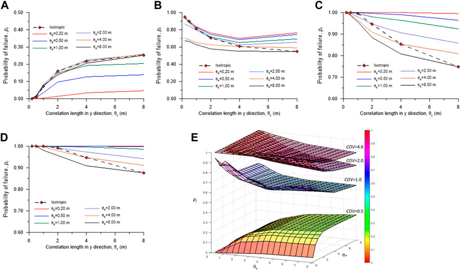
FIGURE 8. The probability of failure with varying $\mathrm{\theta }$: (A) COV = 0.50, (B) COV = 1.00, (C) COV = 2.00, (D) COV = 4.00 and (E) the surface map of distribution of $p_f$ based on different combinations of COV and $\mathrm{\theta }$.

Figure 8E shows the surface map of the 3D distribution of p_f based on different combinations of COV and θ. It can be clearly seen that the p_f surface bends upward when θ increases for low COV, i.e. 0.5. On the other hand, the p_f surface bends upward when θ increases for COV > 1.0. This clearly demonstrates that low COV and high θ may result in higher p_f, whereas high COV and low θ may result in higher p_f. According to Eq. 6, the correlation between the points is calculated by θ. The highest correlation with small θ can be achieved, when the points are closer to each other. In that case, the FOS values from Monte Carlo simulations will be mostly higher than the FOS values and p_f is closer to 0. When the two random points are far away, the correlation can be reduced significantly. A similar observation was found in the study of the isotropic slope by Griffiths and Fenton (2004).

Furthermore, p_f is further investigated by considering COV and dimensionless θ (Θ) in Figure 9. The effect of COV ranges from 0.5 to 8.0 on the failure potential of the slope in isotropic conditions. The probability of slope failure, p_f can increase from less than 20% (COV = 0.5) to near 100% (COV = 8.0). This indicates that the soil with high variability can have a much greater p_f compared with the soil with less variability. It should be noted that the x-axis in Figure 9 presents the dimensionless correlation length, Θ, which is the ratio of spatial correlation length to the slope height. It can be observed that p_f increases with Θ, when COV is less than 1. But this trend changes when COV is more than 1. So, p_f of a soil slope is not affected by a single factor, but by the combination of soil variability and correlation. This should be carefully considered in slope design.

FIGURE 9

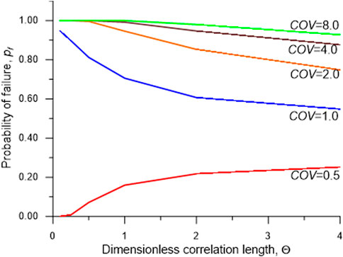
FIGURE 9. Effect of COV and $\mathrm{\theta }$ on the probability of failure in isotropic conditions.

As mentioned previously, this study also considers the effect of soil anisotropy on the probability of slope failure. Figure 10 presents the combined effect of COV and anisotropic θ. In Figure 10A (θ_y = 0.5), the p_f values are almost 1.0, i.e. 100% chance of failure for COV ≥ 2.0. However, when θ_y increases, the p_f values start diverging at high COV (see Figures 10B, C). This observation aligns with the previous discussions that the more correlation length is, the less chance of failure is.

FIGURE 10

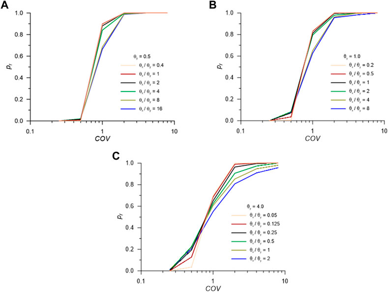
FIGURE 10. Effect of COV and $\mathrm{\theta }$ on the probability of failure in anisotropic conditions: (A) ${\theta }_y=0.5m$, (B) ${\theta }_y=1.0m$ and (C) ${\theta }_y=4.0m$.

In addition, Figure 10 presents the combined effect of the degree of anisotropy (i.e., ratio of θ_x and θ_y) and COV on p_f. Interestingly, the lines representing different degrees of anisotropy crossover each other in Figure 9. Before the crossover, the lower θ_x/θ_y ratio shows a lower p_f. After the crossover, the lower θ_x/θ_y ratio shows a higher p_f. The location of the crossover is highly dependent on the combination of correlation length and COV. For instance, the crossover for θ_y = 0.5 occurs at COV of 0.5, whereas the crossovers for θ_y = 1.0 and 4.0 occur at COV of 0.6 and 0.75 respectively. So, such a reverse effect is clearly dependent on the θ_y and COV. This is an interesting finding that may help in the future study of risk assessment of slope stability. However, it should be aware that other soils with more varying parameter sets (e.g., varying friction angle, stiffness, unit weight, etc.) may be different.

Conclusion

The study introduces a more reliable approach for the quantification of risk in slope design. The combination of a random field generator and FEM (RFEM) considers the variability of soil parameters, which is more realistic than the common deterministic approach. The probability of slope failure is found to be greatly dependent on the statistical variation parameters, namely, COV and θ. This study produces a wide range of different scenarios that can happen in the real design and outputs a set of different p_f values for a slope while the traditional approach assumes a p_f value. Hence, this approach can help to minimise the chance of overestimation or underestimation of slope failure. The effect of anisotropy, which is often neglected in the current engineering practice, is also proposed in this research. In some cases, the p_f values of anisotropic θ are much higher than that of isotropic θ, which helps to prevent possible design failure.

Interestingly, this was found that the combination of a low COV and a high θ may result in a higher p_f, and vice versa. The knowledge from this RFEM study can be adopted in any future research in the risk assessment of geo-structures such as designing a slope of soil with high variability such as tailings. In those cases, the practitioners may consider the additional factor of safety or some possible soil improvement technique to avoid potential failure.

It should be noted that for most natural soils, a reasonable COV range is from 0.1 to 0.5. However, for the materials having very high variability such as tailings, the COV value should be higher.

Data availability statement

The original contributions presented in the study are included in the article/supplementary material, further inquiries can be directed to the corresponding author.

Author contributions

HN: Draft the original version, Software, Methodology, Data analysis, Writing and Editing, Review, Validation, and Visualization. MR: Writing, Supervision, Analysis, Validation, Visualization, Review and Editing. MK: Writing, Analysis, Validation, Review and Editing.

Conflict of interest

The authors declare that the research was conducted in the absence of any commercial or financial relationships that could be construed as a potential conflict of interest.

Publisher’s note

All claims expressed in this article are solely those of the authors and do not necessarily represent those of their affiliated organizations, or those of the publisher, the editors and the reviewers. Any product that may be evaluated in this article, or claim that may be made by its manufacturer, is not guaranteed or endorsed by the publisher.

References

Akbas, B., and Huvaj, N. (2015). “Probabilistic slope stability analyses using limit equilibrium and finite element methods,” in Geotechnical safety and risk V (Amsterdam: IOS Press), 716–721.

Google Scholar

DeGroot, D., and Baecher, G. (1993). Estimating autocovariance of in-situ soil properties. J. Geotechnical Eng. 119 (1), 147–166. doi:10.1061/(asce)0733-9410(1993)119:1(147)

CrossRef Full Text | Google Scholar

Devkota, B., Karim, R., Rahman, M., and Nguyen, H. B. K. (2022). Accounting for expansive soil movement in geotechnical design-a state-of-the-art review. Sustainability 14 (23), 15662.

CrossRef Full Text | Google Scholar

Fenton, G. A., and Griffiths, D. V. (2003). Bearing-capacity prediction of spatially random c – ϕ soils. Can. Geotechnical J. 40 (1), 54–65. doi:10.1139/t02-086

CrossRef Full Text | Google Scholar

Fenton, G. A., and Griffiths, D. V. (2007). “Random field generation and the local average subdivision method,” in Probabilistic methods in geotechnical engineering. Editors D. V. Griffiths, and G. A. Fenton (Vienna: Springer Vienna), 201–223.

Google Scholar

Fenton, G. A., and Griffiths, D. V. (2008). Risk assessment in geotechnical engineering. New Jersey: John Wiley and Sons.

Google Scholar

Fenton, G. A. (1990). Simulation and analysis of random fields. Princeton, New Jersey: Princeton University.

Google Scholar

Fenton, G. A., and Vanmarcke, E. H. (1990). Simulation of random fields via local average subdivision. J. Eng. Mech. 116 (8), 1733–1749. doi:10.1061/(asce)0733-9399(1990)116:8(1733)

CrossRef Full Text | Google Scholar

Gould, S. J. F., Boulaire, F. A., Burn, S., Zhao, X. L., and Kodikara, J. K. (2011). Seasonal factors influencing the failure of buried water reticulation pipes. Water Sci. Technol. 63 (11), 2692–2699. doi:10.2166/wst.2011.507

PubMed Abstract | CrossRef Full Text | Google Scholar

Griffiths, D. (1982). Computation of bearing capacity factors using finite elements. Geotechnique 32 (3), 195–202. doi:10.1680/geot.1982.32.3.195

CrossRef Full Text | Google Scholar

Griffiths, D., and Fenton, G. A. (2004). Probabilistic slope stability analysis by finite elements. J. Geotechnical Geoenvironmental Eng. 130 (5), 507–518. doi:10.1061/(asce)1090-0241(2004)130:5(507)

CrossRef Full Text | Google Scholar

Griffiths, D., and Lane, P. (1999). Slope stability analysis by finite elements. Geotechnique 49 (3), 387–403. doi:10.1680/geot.1999.49.3.387

CrossRef Full Text | Google Scholar

Griffiths, D. V., and Fenton, G. A. (2001). Bearing capacity of spatially random soil: The undrained clay Prandtl problem revisited. Geotechnique 51 (4), 351–359. doi:10.1680/geot.2001.51.4.351

CrossRef Full Text | Google Scholar

Griffiths, D. V., Huang, J., and Fenton, G. A. (2015). “Probabilistic slope stability analysis using RFEM with non-stationary random fields,” in Geotechnical safety and risk V. Editors F. v. T. T. Schweckendiek, D. Pereboom, M. van Staveren, and P. Cools (Amsterdam: IOS Press.), 704–709. The Netherlands.

Google Scholar

Huang, W., Fityus, S., Bishop, D., Smith, D., and Sheng, D. (2006). Finite-element parametric study of the consolidation behavior of a trial embankment on soft clay. Int. J. Geomechanics 6 (5), 328–341. doi:10.1061/(asce)1532-3641(2006)6:5(328)

CrossRef Full Text | Google Scholar

Huang, J., Lyamin, A. V., Griffiths, D. V., Krabbenhoft, K., and Sloan, S. W. (2013). Quantitative risk assessment of landslide by limit analysis and random fields. Comput. Geotechnics 53, 60–67. doi:10.1016/j.compgeo.2013.04.009

CrossRef Full Text | Google Scholar

Idriss, I. M., Dobry, R., and Sing, R. (1978). Nonlinear behavior of soft clays during cyclic loading. J. Geotechnical Geoenvironmental Eng. 104, 1427–1447. ASCE 14265. doi:10.1061/ajgeb6.0000727

CrossRef Full Text | Google Scholar

Jiang, S.-H., Huang, J., Griffiths, D. V., and Deng, Z.-P. (2022a). Advances in reliability and risk analyses of slopes in spatially variable soils: A state-of-the-art review. Comput. Geotechnics 141, 104498. doi:10.1016/j.compgeo.2021.104498

CrossRef Full Text | Google Scholar

Jiang, S.-H., Liu, X., Huang, J., and Zhou, C.-B. (2022b). Efficient reliability-based design of slope angles in spatially variable soils with field data. Int. J. Numer. Anal. Methods Geomechanics 46 (13), 2461–2490. doi:10.1002/nag.3414

CrossRef Full Text | Google Scholar

Karim, M. R., Hughes, D., and Rahman, M. M. (2022). Unsaturated hydraulic conductivity estimation-a case study modelling the soil-atmospheric boundary interaction. Processes 10 (7), 1306.

CrossRef Full Text | Google Scholar

Karim, M. R., Manivannan, G., Gnanendran, C. T., and Lo, S.-C. R. (2011). Predicting the long-term performance of a geogrid-reinforced embankment on soft soil using two-dimensional finite element analysis. Canadian Geotechnical Journal 48 (5), 741–753.

CrossRef Full Text | Google Scholar

Karim, M. R., Rahman, M. M., Nguyen, H. B. K., Cameron, D., Iqbal, A., and Ahenkorah, I. (2021). Changes in thornthwaite moisture index and reactive soil movements under current and future climate scenarios—a case study. Energies 14 (20), 6760. doi:10.3390/en14206760

CrossRef Full Text | Google Scholar

Kasama, K., and Whittle, A. J. (2011). Bearing capacity of spatially random cohesive soil using numerical limit analyses. J. Geotechnical Geoenvironmental Eng. 137 (11), 989–996. doi:10.1061/(asce)gt.1943-5606.0000531

CrossRef Full Text | Google Scholar

Kasama, K., and Whittle, A. J. (2016). Effect of spatial variability on the slope stability using random field numerical limit analyses. Georisk Assess. Manag. Risk Eng. Syst. Geohazards 10 (1), 42–54. doi:10.1080/17499518.2015.1077973

CrossRef Full Text | Google Scholar

Li, J. H., Zhou, Y., Zhang, L. L., Tian, Y., Cassidy, M. J., and Zhang, L. M. (2016). Random finite element method for spudcan foundations in spatially variable soils. Eng. Geol. 205, 146–155. doi:10.1016/j.enggeo.2015.12.019

CrossRef Full Text | Google Scholar

Li, Y., Qian, C., Fu, Z., and Li, Z. (2019). On two approaches to slope stability reliability assessments using the random finite element method. Appl. Sci. 9 (20), 4421. doi:10.3390/app9204421

CrossRef Full Text | Google Scholar

Liu, Y., Zhang, W., Zhang, L., Zhu, Z., Hu, J., and Wei, H. (2018). Probabilistic stability analyses of undrained slopes by 3D random fields and finite element methods. Geosci. Front. 9 (6), 1657–1664. doi:10.1016/j.gsf.2017.09.003

CrossRef Full Text | Google Scholar

Lyamin, A. V., and Sloan, S. W. (2002a). Lower bound limit analysis using non-linear programming. Int. J. Numer. Anal. Methods Geomechanics 55 (5), 573–611. doi:10.1002/nme.511

CrossRef Full Text | Google Scholar

Lyamin, A. V., and Sloan, S. W. (2002b). Upper bound limit analysis using linear finite elements and non-linear programming. Int. J. Numer. Anal. Methods Geomechanics 26 (2), 181–216. doi:10.1002/nag.198

CrossRef Full Text | Google Scholar

Nguyen, H. B. K., and Rahman, M. M. (2015). in Finite element analysis for spatially stochastic soil: Anisotropic studies. Editors M. Iskander, M. T. Suleiman, J. B. Anderson, and D. F. Laefer (Reston, Virginia: American Society of Civil Engineers), 271–278. Geo-Congress 2015.

Google Scholar

Nguyen, T. S., Likitlersuang, S., Tanapalungkorn, W., Phan, T. N., and Keawsawasvong, S. (2022). Influence of copula approaches on reliability analysis of slope stability using random adaptive finite element limit analysis. Int. J. Numer. Anal. Methods Geomechanics 46 (12), 2211–2232. doi:10.1002/nag.3385

CrossRef Full Text | Google Scholar

Pieczyńska-Kozłowska, J. M., Puła, W., Griffiths, D. V., and Fenton, G. A. (2015). Influence of embedment, self-weight and anisotropy on bearing capacity reliability using the random finite element method. Comput. Geotechnics 6, 229–238. doi:10.1016/j.compgeo.2015.02.013

CrossRef Full Text | Google Scholar

Rahman, M. M., and Nguyen, H. B. K. (2012). “Applications of random finite element method in bearing capacity problems,” in Proceedings of the sixth International Conference on Advanced Engineering Computing and Applications in Sciences (ADVCOMP 2012), 53–58.

Google Scholar

Rahman, M. M., and Nguyen, H. B. K. (2013). Spatial variability of material parameter and bearing capacity of clay. Adv. Mater. Res. 629, 433–437. doi:10.4028/www.scientific.net/amr.629.433

CrossRef Full Text | Google Scholar

Shu, S., Ge, B., Wu, Y., and Zhang, F. (2023). Probabilistic assessment on 3D stability and failure mechanism of undrained slopes based on the kinematic approach of limit analysis. Int. J. Geomechanics 23 (1), 06022037. doi:10.1061/(asce)gm.1943-5622.0002635

CrossRef Full Text | Google Scholar

Sloan, S. W., and Kleeman, P. W. (1995). Upper bound limit analysis using discontinuous velocity fields. Comput. Methods Appl. Mech. Eng. 127, 293–314. doi:10.1016/0045-7825(95)00868-1

CrossRef Full Text | Google Scholar

Sloan, S. W. (1988). Lower bound limit analysis using finite elements and linear programming. Int. J. Numer. Anal. Methods Geomechanics 12 (1), 61–77. doi:10.1002/nag.1610120105

CrossRef Full Text | Google Scholar

Smith, I. M., and Griffiths, D. V. (1998). Programming the finite element method. Chichester ; New York: John Wiley and Sons.

Google Scholar

Vanmarcke, E. H. (1984). Random fields: Analysis and sysnthesis. Cambridge: MIT Press.

Google Scholar

Vessia, G., Cherubini, C., Pieczynska, J., and Pula, W. (2009). Application of random finite element method to bearing capacity design of strip footing. J. Geoengin. 4 (3), 103–112.

Google Scholar

Zaskórski, Ł., Puła, W., and Griffiths, D. V. (2017). Bearing capacity assessment of a shallow foundation on a two-layered soil using the random finite element method. Geo-Risk 2017, 468–477.

Google Scholar

Zhu, D., Griffiths, D. V., Huang, J., and Fenton, G. A. (2017). Probabilistic stability analyses of undrained slopes with linearly increasing mean strength. Géotechnique 67 (8), 733–746. doi:10.1680/jgeot.16.p.223

CrossRef Full Text | Google Scholar