Equilibrium path and stability analysis of rigid origami using energy minimization of frame model

This paper presents a method of equilibrium path analysis and stability analysis of an equilibrium state for a rigid origami, which consists of rigid flat faces connected by straight crease lines (folding lines) and can be folded and unfolded without deformation of its faces. This property is well suited to the application to deployable structures and morphing building envelopes consisting of stiff panels. In this study, a frame model which consists of hinges and rigid frame members is used to model the kinematics of a rigid origami. Faces and crease lines of a rigid origami are represented by frame members and hinges, respectively. External loads are applied to the nodes of a frame model, and the displacements of some nodes are fixed. Small rotational stiffness proportional to the length of a crease line is assumed in each hinge to uniquely determine the equilibrium state, which is obtained by solving the optimization problem for minimizing the total potential energy under the conditions so that the displacements of the nodes and the members are compatible. The optimization problem is solved by the augmented Lagrangian method, and the positive definiteness of the Hessian of the augmented Lagrangian is investigated to determine the stability of the equilibrium state. Equilibrium path analyses are carried out and bifurcations of the equilibrium paths are investigated for examples with waterbomb patterns.

1 Introduction

Origami is widely recognized as a traditional play and art form in which one or more pieces of paper are folded to create various two- or three-dimensional shapes. In addition, the continuous transition and the mechanical properties of shapes produced by folding have many engineering applications (Meloni et al., 2021) such as foldable shelters (Lee and Gattas, 2016), shock absorbers (Ma and You, 2013), medical devices (Kuribayashi et al., 2006), and metamaterials (Silverberg et al., 2014). Rigid origami is a kind of polyhedral origami that can be folded and unfolded without deformation of its faces (Tachi, 2010). The deformation mechanism of a rigid origami which is often called a rigid-fold mechanism can be applied to deployable structures consisting of stiff panels connected by hinges (Zirbel et al., 2013), and also to kinematics modeling of robots (Belke and Paik, 2017). Applications in architecture and civil engineering also exist, e.g., the movable sunshade of Al Bahr Towers and Rolling Bridge which can be rolled up (Reis et al., 2015). Rigid origami also has wide potential for the development of new construction methods of roofs and walls with distinctive shapes like the Panta-dome (Kawaguchi, 1991). There are many studies on the kinematics and the mechanical properties of rigid origami. Various techniques such as optimization and graph theory of mathematics and structural engineering are utilized; e.g., simulation of the folding process based on the projection to the constraint space (Tachi, 2009), origami design based on the Bayesian topology optimization (Shende et al., 2021), rigidity analysis based on the theory of combinatorial rigidity (Katoh and Tanigawa, 2011), and assigning mountain or valley fold to each crease line based on graph theory and mixed-integer linear programming (Chen et al., 2020).

It is important to understand the deformation properties to design a structure that can be efficiently and safely deployed by the rigid-fold mechanism. However, the deformation process of rigid origami is very complicated, and it is difficult to obtain an analytical solution because it is generally a multi-degree-of-freedom mechanism except for some special folding patterns such as Miura-ori (Miura and Pellegrino, 2020) shown in Figure 1A. Therefore, a numerical solution is generally used to iteratively obtain the folding states tracing the deformation path, and a rigid origami is regarded as a mechanism consisting of panels connected by hinges. Analysis of the deformation path can be categorized into two types. One is the pure mechanism analysis that considers only geometric constraints based on the assumption that faces are completely rigid. The other is the structural analysis that finds an equilibrium state under external loads or forced displacements assuming rotational stiffness of crease lines (folding lines) and/or elastic deformation of the faces. A path traced by a pair of the load factor and the folding state is called an equilibrium path. There may exist a singular point on a path called a bifurcation point where one or more branching paths exist and a limit point where a snap-through behavior can be observed. Special consideration should be given to these singular points since the degrees of freedom of the mechanism may change at these points. In the analysis of pure mechanisms, it has been shown that the second-order or higher-order terms are necessary at the singular point to trace the path (Salerno, 1992; Tachi, 2012; Demaine et al., 2016). Besides, in the analysis of an equilibrium path, various studies exist based on the general theory of elastic stability (Thompson and Hunt, 1973; Gillman et al., 2018). Although there are many studies on mechanisms and equilibrium path analysis, the method for investigating the equilibrium path of a rigid origami with strictly rigid faces is rarely studied. This hybrid analysis of the pure mechanism and the structural analysis is important to understand the foldability (Tachi and Hull, 2017) of a crease pattern and for the prototyping of the deployable structure using a rigid-fold mechanism.

FIGURE 1

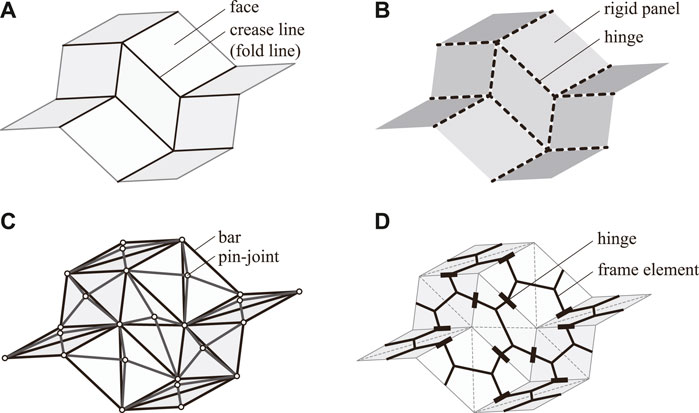
FIGURE 1. Numerical models representing Miura-ori for the analysis of kinematics of rigid origami. (A) Crease pattern of Miura-ori. (B) Rotational hinge model. (C) Truss model. (D) Frame model.

It is also important to develop a numerical model suitable for the analysis of a rigid origami. In the study of kinematics of a rigid origami, a rotational hinge model shown in Figure 1B and a truss model shown in Figure 1C are often used. A rotational hinge model represents the folding state of a rigid origami using the folding angles of the crease lines (Tachi, 2009; Watanabe, 2018). The positions of the vertices are computed from the complicated nonlinear equations of the folding angles and the inner angles of faces. Therefore, a rotational hinge model has a disadvantage for the analysis with the constraints on the displacements of vertices, and it is usually used for pure mechanism analysis. Rigid Origami Simulator¹ by Tachi (2009) can trace an exact rigid-fold deformation path without deformation of faces. Although the study on the equilibrium of a rotational hinge model is also provided by He and Guest (2022), the physical interpretation of the loads and the internal forces considered in their study are torques applied at crease lines; this makes it difficult to understand the equilibrium state intuitively. On the other hand, a rigid origami is represented by pin-jointed bars in a truss model, where the nodal coordinates are the variables. The rigidity of each face can be guaranteed by simply placing the rigid bars along the edges for the rigid origami with only triangular faces. However, to constrain the in-plane and out of plane deformation of faces with more than three edges, it is necessary to constrain the nodal displacements (Schenk and Guest, 2011; Filipov et al., 2017) or to introduce diagonal bars and construct a bar-joint structure in a three-dimensional manner (Saito et al., 2015; Zhang et al., 2018), which tends to make the model complicated. Since the nodes of the truss model are located at the vertices of the origami, it is easy to incorporate the constraints on the nodal displacements and the equilibrium with nodal loads. Therefore, it is often used for the analysis of the equilibrium path under the external loads or the forced displacements; e.g., MERLIN2² by Liu and Paulino (2018) and Origami Simulator³ by Ghassaei et al. (2018). However, they allow deformation of the faces of a rigid origami, and an exact rigid-fold path may not be obtained. An exact rigid-fold path reflecting the equilibrium can be obtained by the method proposed by Li (2020), although the equilibrium condition is not strictly satisfied. The conventional FE methods using shell elements are also often used for the elastic analysis of rigid origami. They are suited to the analysis of detailed mechanical properties of rigid origami, such as local deformation, but are not as suited as elastic truss models to tracing the exact rigid-fold path.

To overcome the difficulty in a rotational hinge model, a truss model, and a FE model as mentioned above, the authors have proposed a frame model (Hayakawa and Ohsaki, 2019a; b, 2021) shown in Figure 1D based on the concept of a partially rigid frame (Tsuda et al., 2013; Ohsaki et al., 2016; Watada and Ohsaki, 2018). Frame members are connected by hinges whose axes are parallel to the crease lines, and rigidly connected on the faces. Details of the configuration of a frame model are shown in Section 2.1. A frame model is used for the analysis with the assumption that the faces of a rigid origami is completely rigid, and the exact rigid-fold path can be obtained. However, it cannot represent elastic deformation of the faces, which can be represented by FE methods using shell elements. A frame model has the advantage of being able to represent a rigid origami with a simpler configuration than a rotational hinge model and a truss model. Analysis with boundary conditions can be easily performed compared to a rotational hinge model since the nodal coordinates are variables in the frame model. In addition, there is no need to constrain nodal displacements or arrange members three-dimensionally, as is the case with a truss model, to constrain the deformation of faces with more than three edges since each face is composed of multiple rigidly-joined frame elements.

In this study, the frame model is utilized to perform an equilibrium path analysis and stability analysis of equilibrium state when an external load is applied to a rigid origami. As in most equilibrium path analyses using truss models, rotational springs are introduced at the hinges of the frame model to stabilize the equilibrium under nodal loads. The proposed method in this paper has the following features.

• By incorporating the rotational stiffness of the hinges, the deformation path is uniquely determined except for the possible existence of singular points. This enables us to avoid the difficulty in tracing the deformation path caused by many multiple bifurcation points (Ohsaki and Ikeda, 2006, 2007) which may exist on the deformation path if the rotation stiffnesses of the hinges are not incorporated.

• Instead of solving the equilibrium equations directly, the equilibrium state is obtained by minimizing the total potential energy. This enables us to use the stability theories based on the energy principle and to obtain the equilibrium state by utilizing sophisticated optimization techniques.

• The total potential energy minimization problem with the compatibility equations of the mechanism is solved by the augmented Lagrangian method (Hestenes, 1969; Birgin and Martínez, 2012), which often has better convergence than the conventional Lagrangian and penalty methods.

• Stability analysis of the equilibrium state is performed by eigenvalue analysis of the Hessian matrix of the augmented Lagrangian.

The structure of this paper is as follows. Section 2 shows the configuration of a frame model and the formulation of the compatibility equations for a frame model. In Section 3, a method of equilibrium path analysis under nodal loads is presented using the augmented Lagrangian method. Examples of equilibrium path and stability analyses using the proposed method are shown in Section 4. First, the analysis of a two-dimensional two-member model which can analytically determine the singularity on the equilibrium path is performed to confirm that the proposed method can accurately detect the singularity phenomenon. Then, the analysis is carried out for a waterbomb cell that has a single inner vertex and multiple degrees of freedom of rigid-fold mechanism. A waterbomb cell is a well-known rigid-foldable pattern that has a multi-degrees of freedom mechanism, and there are some examples of the deformation path analyses including a bifurcation and a limit point; e.g., Gillman et al. (2018). However, the stability of a fully developed flat state and a bifurcation path from the flat state have not been investigated well. The flat state is a singular point on the deformation path of a rigid origami as pointed out in Tachi (2012), and the degrees of freedom of the mechanism decreases when the out-of-plane deformation occurs. In this paper, the stabilities and the equilibrium paths of the flat states with two types of boundary and load conditions are investigated. Note that the equilibrium path can be determined uniquely by the rotational springs although the waterbomb cell has the multiple degrees of freedom mechanism. The possible existence of the multiple bifurcation at the flat states investigated in Chen and Santangelo (2018) also can be avoided by assigning the initial imperfection in addition to the rotational springs. Finally, the conclusions of this paper are given in Section 5.

2 Frame model for the analysis of a rigid origami

In this section, the configuration and the compatibility conditions of a frame model are shown. The compatibility conditions are derived based on Watada and Ohsaki (2018) and Géradin and Cardona (2007). They are formulated with respect to the generalized displacements including translational and rotational displacements of nodes and members and rotation angles of hinges.

2.1 Configuration of a frame model

A frame model is a kind of partially rigid frame (Tsuda et al., 2013; Ohsaki et al., 2016; Watada and Ohsaki, 2018) representing a rigid origami mechanism (Hayakawa and Ohsaki, 2019a; b, 2021). Figure 2 shows an example of Miura-ori modeled by a frame model. A frame model consists of nodes, members (frame elements), and hinges. The basic structure of a frame model is shown by gray bold lines in Figure 2 which represents a shape of the rigid origami, and nodes and members shown by blue bold lines are added to apply loads and boundary conditions. A face with more than three edges is divided into triangles by the dividing edges. Basically, nodes are located at the center points of crease lines, perimeters, and dividing edges and at the barycenters of triangular faces. As shown by gray in Figure 2B, two members are connected to the node on a crease line in the basic structure of a frame model, and a member is connected to the node rigidly and another member is connected to the node via a hinge. In this study, the member end connected to a node rigidly is called the rigid end, and the member end connected via a hinge is called the hinged end. The axis of each hinge coincides with the corresponding crease line. The additional nodes are placed at the vertices to which the loads or the boundary conditions are applied, and the additional members shown in blue in Figure 2 are placed along the edges which have rigid ends. The positions of the vertices of a rigid origami where the additional nodes do not exist can be calculated by the positions of nodes on the edges. Details of the calculation of the positions of vertices can be found in Hayakawa and Ohsaki (2021).

FIGURE 2

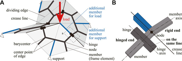
FIGURE 2. Detailed configuration of a frame model. (A) Overall view. (B) Enlarged view of the region surrounded by dotted lines in the overall view.

2.2 Compatibility condition at the rigid end

The number of nodes, members, and hinges are denoted by n_N, n_M, and n_H, respectively. As shown in Figure 3, the translation vector of the center point of member i (= 1, … , n_M) in the global coordinate system (x₁, x₂, x₃) is denoted by ${\mathbf{V}}_i={(V_i^{(1)},V_i^{(2)},V_i^{(3)})}^{\mathsf{T}}\in {\mathbb{R}}^3$, and the rotation vector is denoted by ${\mathbf{\Psi }}_i={({\mathrm{\Psi }}_i^{(1)},{\mathrm{\Psi }}_i^{(2)},{\mathrm{\Psi }}_i^{(3)})}^{\mathsf{T}}\in {\mathbb{R}}^3$. Let ${\mathbf{r}}_{ij}\in {\mathbb{R}}^3$ denote the vector directing from the center point to the j-th end (j = 1, 2) of member i at the initial configuration. Defining $\mathbf{R}({\mathbf{\Psi }}_i)\in {\mathbb{R}}^{3\times 3}$ to be the Rodrigues’ rotation matrix (Géradin and Cardona, 2007) with respect to the rotation vector Ψ_i, the vector obtained by rotating r_ij with member i can be represented as R (Ψ_i) r_ij. The Rodrigues’ rotation matrix R (Ψ_i) is defined as follows:

$\mathbf{R}\left({\mathbf{\Psi }}_i\right)=\cos \left(\Vert {\mathbf{\Psi }}_i\Vert \right){\mathbf{I}}_3+\frac{1}{\Vert {\mathbf{\Psi }}_i{\Vert }^2}\left\{1-\cos \left(\Vert {\mathbf{\Psi }}_i\Vert \right)\right\}{\mathbf{\Psi }}_i{{\mathbf{\Psi }}_i}^{\mathsf{T}}+\frac{1}{\Vert {\mathbf{\Psi }}_i\Vert }\sin \left(\Vert {\mathbf{\Psi }}_i\Vert \right){\left[{\mathbf{\Psi }}_i\right]}_{\times }(1)$

where ${\mathbf{I}}_3\in {\mathbb{R}}^3$ is the identity matrix and ${[{\mathbf{\Psi }}_i]}_{\times }$ represents the cross-product matrix with respect to Ψ_i, which is defined as follows:

${\left[{\mathbf{\Psi }}_i\right]}_{\times }=\left[\begin{array}{ccc}\hfill 0\hfill & \hfill -{\mathrm{\Psi }}_i^{\left(3\right)}\hfill & \hfill {\mathrm{\Psi }}_i^{\left(2\right)}\hfill \\ \hfill {\mathrm{\Psi }}_i^{\left(3\right)}\hfill & \hfill 0\hfill & \hfill -{\mathrm{\Psi }}_i^{\left(1\right)}\hfill \\ \hfill -{\mathrm{\Psi }}_i^{\left(2\right)}\hfill & \hfill {\mathrm{\Psi }}_i^{\left(1\right)}\hfill & \hfill 0\hfill \end{array}\right]$

The detailed calculation of Eq. 1 is shown in Supplementary Material S1. Let ${\mathbf{U}}_k={(U_k^{(1)},U_k^{(2)},U_k^{(3)})}^{\mathsf{T}}\in {\mathbb{R}}^3$ and ${\mathbf{\Theta }}_k={({\mathrm{\Theta }}_k^{(1)},{\mathrm{\Theta }}_k^{(2)},{\mathrm{\Theta }}_k^{(3)})}^{\mathsf{T}}\in {\mathbb{R}}^3$ denote the translation and rotation vectors of node k (= 1, … , n_N), respectively. When j-th end of member i is connected to node k, the following equation should be satisfied because the translation of the member end is equal to the translation of the node:

${\mathbf{U}}_k-{\mathbf{V}}_i-\left\{\mathbf{R}\left({\mathbf{\Psi }}_i\right)-{\mathbf{I}}_3\right\}{\mathbf{r}}_{ij}=\mathbf{0}(2)$

In addition, if member i is rigidly connected to node k, the rotation of member i is equal to the rotation of node k, and the following equation should be satisfied:

${\mathbf{\Theta }}_k-{\mathbf{\Psi }}_i=\mathbf{0}(3)$

FIGURE 3

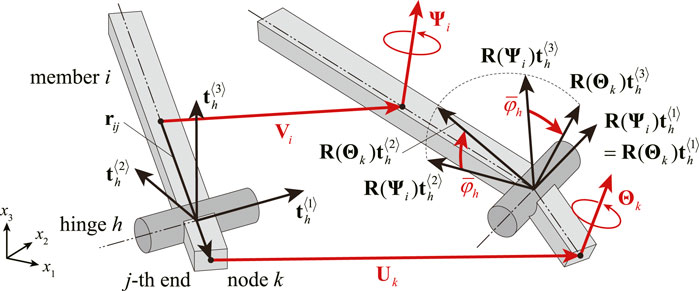
FIGURE 3. Displacements of member i and node k and rotation angle of hinge h.

2.3 Compatibility condition at the hinged end

As shown in Figure 3, the unit vector parallel to the rotation axis of hinge h (= 1, … , n_H) at the undeformed state in the global coordinate system (x₁, x₂, x₃) is denoted by ${\mathbf{t}}_h^{⟨1⟩}\in {\mathbb{R}}^3$. ${\mathbf{t}}_h^{⟨2⟩}$ and ${\mathbf{t}}_h^{⟨3⟩}\in {\mathbb{R}}^3$ are defined as the unit vectors satisfying the following equations:

$\begin{array}{ll}\hfill {\mathbf{t}}_h^{\langle 1\rangle }\times {\mathbf{t}}_h^{\langle 2\rangle }& ={\mathbf{t}}_h^{\langle 3\rangle }\hfill \\ \hfill {\mathbf{t}}_h^{\langle 2\rangle }\times {\mathbf{t}}_h^{\langle 3\rangle }& ={\mathbf{t}}_h^{\langle 1\rangle }\hfill \end{array}$

Then, the reference frame of hinge h in the undeformed state is represented by the three vectors ${\mathbf{t}}_h^{⟨l⟩}$ (l = 1, 2, 3). Consider the case where the j-th end of member i is connected to node k via hinge h. The translation between the center point of member i and node k satisfies Eq. 2. Since the relative rotation of member i and node k is constrained except around the rotation axis of hinge h as shown in Figure 3, the following equations hold:

$\left(\mathbf{R}\left({\mathbf{\Psi }}_i\right){\mathbf{t}}_h^{\langle 1\rangle }\right)\cdot \left(\mathbf{R}\left({\mathbf{\Theta }}_k\right){\mathbf{t}}_h^{\langle 2\rangle }\right)=0\left(\mathbf{R}\left({\mathbf{\Psi }}_i\right){\mathbf{t}}_h^{\langle 1\rangle }\right)\cdot \left(\mathbf{R}\left({\mathbf{\Theta }}_k\right){\mathbf{t}}_h^{\langle 3\rangle }\right)=0(4)$

Let φ_h denote the increment of the rotation angle of hinge h due to the deformation of the structure. φ_h is treated as an independent variable to simplify the calculation of the total potential energy and its derivatives introduced in Section 3.3. Note that φ_h is not a variable in Watada and Ohsaki (2018), and it is calculated from the displacements of the node and the center point of the member. When Ψ_i and Θ_k satisfy Eq. 4 and $\mathbf{R}({\mathbf{\Psi }}_i){\mathbf{t}}_h^{⟨1⟩}$ and $\mathbf{R}({\mathbf{\Theta }}_k){\mathbf{t}}_h^{⟨1⟩}$ always coincide during the deformation process, the ideal value of φ_h which is denoted by ${\bar{\phi }}_h$ and shown in Figure 3 can be determined from the following equations:

$\sin {\bar{\phi }}_h=\left(\mathbf{R}\left({\mathbf{\Psi }}_i\right){\mathbf{t}}_h^{\langle 3\rangle }\right)\cdot \left(\mathbf{R}\left({\mathbf{\Theta }}_k\right){\mathbf{t}}_h^{\langle 2\rangle }\right)=-\left(\mathbf{R}\left({\mathbf{\Psi }}_i\right){\mathbf{t}}_h^{\langle 2\rangle }\right)\cdot \left(\mathbf{R}\left({\mathbf{\Theta }}_k\right){\mathbf{t}}_h^{\langle 3\rangle }\right)(5)$

$\cos {\bar{\phi }}_h=\left(\mathbf{R}\left({\mathbf{\Psi }}_i\right){\mathbf{t}}_h^{\langle 2\rangle }\right)\cdot \left(\mathbf{R}\left({\mathbf{\Theta }}_k\right){\mathbf{t}}_h^{\langle 2\rangle }\right)=\left(\mathbf{R}\left({\mathbf{\Psi }}_i\right){\mathbf{t}}_h^{\langle 3\rangle }\right)\cdot \left(\mathbf{R}\left({\mathbf{\Theta }}_k\right){\mathbf{t}}_h^{\langle 3\rangle }\right)(6)$

Therefore, assuming that $|{\phi }_h-{\bar{\phi }}_h|<2\pi$ holds throughout the deformation process, the compatibility equation for φ_h can be expressed as follows (Géradin and Cardona, 2007):

$\begin{array}{ll}\hfill & \sin \left({\phi }_h-{\bar{\phi }}_h\right)=0\hfill \\ \hfill \iff & \left\{\left(\mathbf{R}\left({\mathbf{\Psi }}_i\right){\mathbf{t}}_h^{⟨2⟩}\right)\cdot \left(\mathbf{R}\left({\mathbf{\Theta }}_k\right){\mathbf{t}}_h^{⟨2⟩}\right)\right\}\sin {\phi }_h+\left\{\left(\mathbf{R}\left({\mathbf{\Psi }}_i\right){\mathbf{t}}_h^{⟨2⟩}\right)\cdot \left(\mathbf{R}\left({\mathbf{\Theta }}_k\right){\mathbf{t}}_h^{⟨3⟩}\right)\right\}\cos {\phi }_h=0\hfill \\ \hfill \iff & \left(\mathbf{R}\left({\mathbf{\Psi }}_i\right){\mathbf{t}}_h^{⟨2⟩}\right)\cdot \left\{\sin {\phi }_h\left(\mathbf{R}\left({\mathbf{\Theta }}_k\right){\mathbf{t}}_h^{⟨2⟩}\right)+\cos {\phi }_h\left(\mathbf{R}\left({\mathbf{\Theta }}_k\right){\mathbf{t}}_h^{⟨3⟩}\right)\right\}=0\hfill \end{array}(7)$

The left-hand side of Eqs 4, 7 are simply represented by the functions of Ψ_i, Θ_k, and φ_h as follows:

$\begin{array}{ll}\hfill {\mathrm{\Phi }}_{ij}^{\left(1\right)}\left({\mathbf{\Psi }}_i,{\mathbf{\Theta }}_k,{\phi }_h\right)& =\left(\mathbf{R}\left({\mathbf{\Psi }}_i\right){\mathbf{t}}_h^{⟨1⟩}\right)\cdot \left(\mathbf{R}\left({\mathbf{\Theta }}_k\right){\mathbf{t}}_h^{⟨2⟩}\right)\hfill \\ \hfill {\mathrm{\Phi }}_{ij}^{\left(2\right)}\left({\mathbf{\Psi }}_i,{\mathbf{\Theta }}_k,{\phi }_h\right)& =\left(\mathbf{R}\left({\mathbf{\Psi }}_i\right){\mathbf{t}}_h^{⟨1⟩}\right)\cdot \left(\mathbf{R}\left({\mathbf{\Theta }}_k\right){\mathbf{t}}_h^{⟨3⟩}\right)\hfill \\ \hfill {\mathrm{\Phi }}_{ij}^{\left(3\right)}\left({\mathbf{\Psi }}_i,{\mathbf{\Theta }}_k,{\phi }_h\right)& =\left(\mathbf{R}\left({\mathbf{\Psi }}_i\right){\mathbf{t}}_h^{⟨2⟩}\right)\cdot \left\{\sin {\phi }_h\left(\mathbf{R}\left({\mathbf{\Theta }}_k\right){\mathbf{t}}_h^{⟨2⟩}\right)+\cos {\phi }_h\left(\mathbf{R}\left({\mathbf{\Theta }}_k\right){\mathbf{t}}_h^{⟨3⟩}\right)\right\}\hfill \end{array}(8)$

From Eqs 4, 7, when the j-th end of member i is connected to node k via hinge h, the rotations of member i and node k and the change of the rotation angle of hinge h satisfy the following equations:

${\mathbf{\Phi }}_{ij}\left({\mathbf{\Psi }}_i,{\mathbf{\Theta }}_k,{\phi }_h\right)=\left(\begin{array}{c}\hfill {\mathrm{\Phi }}_{ij}^{\left(1\right)}\left({\mathbf{\Psi }}_i,{\mathbf{\Theta }}_k,{\phi }_h\right)\hfill \\ \hfill {\mathrm{\Phi }}_{ij}^{\left(2\right)}\left({\mathbf{\Psi }}_i,{\mathbf{\Theta }}_k,{\phi }_h\right)\hfill \\ \hfill {\mathrm{\Phi }}_{ij}^{\left(3\right)}\left({\mathbf{\Psi }}_i,{\mathbf{\Theta }}_k,{\phi }_h\right)\hfill \end{array}\right)=\mathbf{0}(9)$

2.4 Compatibility equations for the entire structure

The compatibility equations of a frame model with respect to the generalized displacements are formulated by summarizing the compatibility equations formulated in Sections 2.2, 2.3. Let n_B denote the number of fixed degrees of freedom of the nodal displacements. The components of nodal displacements U_k and Θ_k that are not constrained are collected for all nodes to $\mathbf{U}\in {\mathbb{R}}^{6n_{\text{N}}-n_{\text{B}}}$, and the components of member displacements V_i and Ψ_i for all members are collected to $\mathbf{V}\in {\mathbb{R}}^{6n_{\text{M}}}$. In addition, let $\mathit{\phi }\in {\mathbb{R}}^{n_{\text{H}}}$ denote the vector consisting of φ_h, which is the amount of change in the rotation angle of the hinge. The generalized displacement vector is defined as the assemblage of U, V, and φ as $\mathbf{W}={({\mathbf{U}}^{\mathsf{T}},{\mathbf{V}}^{\mathsf{T}},{\mathit{\phi }}^{\mathsf{T}})}^{\mathsf{T}}\in {\mathbb{R}}^{n_{\text{D}}}$. The number of components of W is calculated as n_D = 6n_N − n_B + 6n_M + n_H. Note again that although φ is not included in the generalized displacement vector in the formulation of Watada and Ohsaki (2018), it is included in this paper to simplify the formulation of the total potential energy to be described in Section 3. According to Eqs 2, 3, 9, when the j-th end of member i is connected to node k rigidly or via hinge h, translational and rotational incompatibility vectors represented by $\mathrm{\Delta }{\mathbf{U}}_{ij}\in {\mathbb{R}}^3$ and $\mathrm{\Delta }{\mathbf{\Theta }}_{ij}\in {\mathbb{R}}^3$, respectively, are defined as follows:

$\mathrm{\Delta }{\mathbf{U}}_{ij}={\mathbf{U}}_k-{\mathbf{V}}_i-\left(\mathbf{R}\left({\mathbf{\Psi }}_i\right)-{\mathbf{I}}_3\right){\mathbf{r}}_{ij}(10)$

$\mathrm{\Delta }{\mathbf{\Theta }}_{ij}=\left\{\begin{array}{cc}{\mathbf{\Theta }}_k-{\mathbf{\Psi }}_i\hfill & (\mathrm{Rigidly\; connected})\hfill \\ {\mathbf{\Phi }}_{ij}\left({\mathbf{\Psi }}_i,{\mathbf{\Theta }}_k,{\phi }_h\right)\hfill & (\mathrm{Connected\; by\; hinge}h)\hfill \end{array}\right.(11)$

In Eqs 10, 11, the components of fixed nodal displacements are assumed to be equal to 0. The translational and rotational incompatibility vectors ΔU_ij and ΔΘ_ij are combined into the incompatibility vector $\mathbf{C}(\mathbf{W})\in {\mathbb{R}}^{n_{\text{C}}}$ as the nonlinear function of the generalized displacement vector W. Accordingly, the compatibility equations are represented as follows:

$\mathbf{C}\left(\mathbf{W}\right)=\mathbf{0}(12)$

Since the compatibility equations should be satisfied at all member ends, the number of components of C(W) is n_C = 12n_M.

3 Energy minimization for equilibrium path analysis

This section presents an energy minimization approach to the analysis of the equilibrium path and stability of the equilibrium state when nodal loads are applied to a frame model with rotational springs introduced at the hinges. Assuming that the members of the frame are rigid, the equilibrium state is derived by minimizing the total potential energy consisting of the strain energy of springs and the work by the nodal loads. In this paper, we call the pair (W, Λ) the equilibrium point where Λ is a load factor and W is the corresponding generalized displacement vector which minimizes the total potential energy. An equilibrium path is a curve in the space of the load factor and the generalized displacements which is the trajectory drawn by the equilibrium points. Stability analysis of the equilibrium state is also performed based on the stability condition at the stationary point of the total potential energy. In the following, the reference generalized displacement for calculating the total potential energy is W = 0. The initial displacement for the analysis is assigned as $\mathbf{W}={\mathbf{W}}_0={({\mathbf{U}}_0^{\mathsf{T}},{\mathbf{V}}_0^{\mathsf{T}},{\mathit{\phi }}_0^{\mathsf{T}})}^{\mathsf{T}}$.

3.1 Energy minimization problem

The nodal load vector corresponding to the free degrees of freedom of the nodal displacement is represented as ΛP_U where ${\mathbf{P}}_{\text{U}}\in {\mathbb{R}}^{6n_{\text{N}}-n_{\text{B}}}$ is a constant vector. The residual rotation angles of the springs at the hinges are considered at the initial state W = W₀, and the assemblage of them is represented by $\tilde{\mathit{\phi }}\in {\mathbb{R}}^{n_{\text{H}}}$. Therefore, the rotation angles of the springs at W can be denoted by $\mathit{\phi }-\tilde{\mathit{\phi }}$. If they are set to zero at W = W₀, $\tilde{\mathit{\phi }}$ is assigned as $\tilde{\mathit{\phi }}={\mathit{\phi }}_0$. Defining ${\mathbf{K}}_{\text{H}}\in {\mathbb{R}}^{n_{\text{H}}\times n_{\text{H}}}$ as the diagonal matrix whose diagonal component is the rotational stiffness of the spring at each hinge, the total potential energy with the constant load factor Λ is defined as ${\mathrm{\Pi }}_{\mathrm{\Lambda }}^{\rho }(\mathit{\rho },\mathbf{U})$ which is the function of φ and U as follows:

${\mathrm{\Pi }}_{\mathrm{\Lambda }}^{\phi }\left(\mathit{\phi },\mathbf{U}\right)=\frac{1}{2}{\left(\mathit{\phi }-\tilde{\mathit{\phi }}\right)}^{\mathsf{T}}{\mathbf{K}}_{\text{H}}\left(\mathit{\phi }-\tilde{\mathit{\phi }}\right)-{\mathbf{U}}^{\mathsf{T}}\left(\mathrm{\Lambda }{\mathbf{P}}_{\text{U}}\right)(13)$

Note again that the reference generalized displacement for calculating the total potential energy is W = 0. Incorporating $\mathbf{W}={({\mathbf{U}}^{\mathsf{T}},{\mathbf{V}}^{\mathsf{T}},{\mathit{\phi }}^{\mathsf{T}})}^{\mathsf{T}}$, the total potential energy can be reformulated as the function of W as follows:

${\mathrm{\Pi }}_{\mathrm{\Lambda }}\left(\mathbf{W}\right)=\frac{1}{2}{\left(\mathbf{W}-\tilde{\mathbf{W}}\right)}^{\mathsf{T}}\mathbf{K}\left(\mathbf{W}-\tilde{\mathbf{W}}\right)-{\mathbf{W}}^{\mathsf{T}}\left(\mathrm{\Lambda }\mathbf{P}\right)(14)$

where $\tilde{\mathbf{W}}$, P, and K are the constant vectors and a matrix defined as follows:

$\begin{array}{ll}\hfill \tilde{\mathbf{W}}& =\left(\begin{array}{c}\hfill {\mathbf{0}}_{n_{\text{D}}-n_{\text{H}}}\hfill \\ \hfill \tilde{\mathit{\phi }}\hfill \end{array}\right)\in {\mathbb{R}}^{n_{\text{D}}}\hfill \\ \hfill \mathbf{P}& =\left(\begin{array}{c}\hfill {\mathbf{P}}_{\text{U}}\hfill \\ \hfill {\mathbf{0}}_{6n_{\text{M}}+n_{\text{H}}}\hfill \end{array}\right)\in {\mathbb{R}}^{n_{\text{D}}}\hfill \\ \hfill \mathbf{K}& =\left[\begin{array}{cc}\hfill {\mathbf{O}}_{\left(n_{\text{D}}-n_{\text{H}}\right)\times \left(n_{\text{D}}-n_{\text{H}}\right)}\hfill & \hfill {\mathbf{O}}_{\left(n_{\text{D}}-n_{\text{H}}\right)\times n_{\text{H}}}\hfill \\ \hfill {\mathbf{O}}_{n_{\text{H}}\times \left(n_{\text{D}}-n_{\text{H}}\right)}\hfill & \hfill {\mathbf{K}}_{\text{H}}\hfill \end{array}\right]\in {\mathbb{R}}^{n_{\text{D}}\times n_{\text{D}}}\hfill \end{array}$

The equilibrium state under the constant nodal load ΛP_U without deformation of members is obtained as the solution (stationary point) of the following optimization problem:

$\left\{\begin{array}{cccc}\hfill & \underset{\mathbf{W}}{\text{min.}}\hfill & \hfill & {\mathrm{\Pi }}_{\mathrm{\Lambda }}\left(\mathbf{W}\right)\hfill \\ \hfill & \text{s.t.}\hfill & \hfill & \mathbf{C}\left(\mathbf{W}\right)=\mathbf{0}\hfill \end{array}\right.(15)$

Although general contact between nodes and members is not considered in this study, it is confirmed that no contact occurs at each equilibrium point of the examples shown in Section 4.

3.2 Equilibrium path analysis

In this section, a procedure of equilibrium path analysis is presented. Equilibrium points are iteratively obtained by solving problem (15) while updating the load factor. First, the process of the augmented Lagrangian method (ALM) (Hestenes, 1969; Birgin and Martínez, 2012) for solving problem (15) is presented. Let $s\in \mathbb{R}$ denote the positive penalty parameter, and the augmented Lagrangian L_s (W, λ) is defined as follows:

$\begin{array}{ll}\hfill L_s\left(\mathbf{W},\mathit{\lambda }\right)& ={\mathrm{\Pi }}_{\mathrm{\Lambda }}\left(\mathbf{W}\right)+\mathbf{C}{\left(\mathbf{W}\right)}^{\mathsf{T}}\mathit{\lambda }+\frac{s}{2}\mathbf{C}{\left(\mathbf{W}\right)}^{\mathsf{T}}\mathbf{C}\left(\mathbf{W}\right)\hfill \\ \hfill & =\frac{1}{2}{\left(\mathbf{W}-\tilde{\mathbf{W}}\right)}^{\mathsf{T}}\mathbf{K}\left(\mathbf{W}-\tilde{\mathbf{W}}\right)-{\mathbf{W}}^{\mathsf{T}}\left(\mathrm{\Lambda }\mathbf{P}\right)+\mathbf{C}{\left(\mathbf{W}\right)}^{\mathsf{T}}\left(\mathit{\lambda }+\frac{s}{2}\mathbf{C}\left(\mathbf{W}\right)\right)\hfill \end{array}(16)$

Defining $\mathbf{\Gamma }(\mathbf{W})={\nabla }_{\text{W}}\mathbf{C}(\mathbf{W})\in {\mathbb{R}}^{n_{\text{C}}\times n_{\text{D}}}$, the gradient of L_s (W, λ) with respect to W and λ can be calculated, respectively, as follows:

${\nabla }_{\text{W}}{L}_s\left(\mathbf{W},\mathit{\lambda }\right)=\mathbf{K}\left(\mathbf{W}-\tilde{\mathbf{W}}\right)-\mathrm{\Lambda }\mathbf{P}+\mathbf{\Gamma }{\left(\mathbf{W}\right)}^{\mathsf{T}}\left(\mathit{\lambda }+s\mathbf{C}\left(\mathbf{W}\right)\right)(17)$

${\nabla }_{\lambda }{L}_s\left(\mathbf{W},\mathit{\lambda }\right)=\mathbf{C}\left(\mathbf{W}\right)(18)$

Γ(W) is called the compatibility matrix, and the degrees of kinematic indeterminacy of the frame model can be calculated as n_D − rank Γ(W). In addition, the degrees of statical indeterminacy can be calculated as n_C − rank Γ(W) (Tsuda et al., 2013; Watada and Ohsaki, 2018). The detailed calculation of Γ(W) is shown in Supplementary Material S2. When W* and λ* are the solution and the corresponding Lagrange multiplier, respectively, of problem (15), the following equations hold:

${\nabla }_{\text{W}}{L}_s\left({\mathbf{W}}^{\ast },{\mathit{\lambda }}^{\ast }\right)=\mathbf{0}(19)$

${\nabla }_{\lambda }{L}_s\left({\mathbf{W}}^{\ast },{\mathit{\lambda }}^{\ast }\right)=\mathbf{C}\left({\mathbf{W}}^{\ast }\right)=\mathbf{0}(20)$

Hence, W* is the solution to the following optimization problem with λ = λ*:

$\underset{\mathbf{W}}{\text{min.}}{L}_s\left(\mathbf{W},\mathit{\lambda }\right)(21)$

Conversely, if $\bar{\mathbf{W}}$ satisfies the compatibility equation (12) and is the solution to problem (21), $\bar{\mathbf{W}}$ is obviously the solution to problem (15) since the stationary conditions of problem (15) are satisfied. Therefore, instead of solving the optimization problem (15) directly, we can solve the optimization problem (21) and check that the solution satisfies the constraints to obtain the equilibrium point. Since the appropriate Lagrange multiplier λ* corresponding to the solution to problem (15) is unknown, λ* is estimated by iteratively solving problem (21) while updating λ as follows:

$\mathit{\lambda }\leftarrow \mathit{\lambda }+s\mathbf{C}\left(\bar{\mathbf{W}}\right)$

The value of penalty parameter s is automatically adjusted in the process of the ALM by the algorithm proposed by Birgin and Martínez (2012). The maximum absolute value among the components of C(W) can be restricted below the tolerance ϵ_tol > 0 by their algorithm. The procedure of the ALM is provided in Supplementary Material S3. The ALM has good global convergence property and robustness under the degenerate constraints, and thus there is some flexibility in the choice of the initial value of λ (Izmailov and Solodov, 2015).

The equilibrium path is estimated by successively solving problem (15) by the ALM while updating the load factor as Λ ←Λ + dΛ (dΛ > 0), i.e., the equilibrium path is traced by the incremental loading analysis. The equilibrium path analysis starts from Λ = 0 and continues until one of the following termination conditions is satisfied:

• The specified component W_i of W reaches the target $W_i^{\text{max}}$ or $W_i^{\text{min}}$ $(W_i^{\text{min}}<W_i^{\text{max}})$.

• The load factor Λ is greater than the specified maximum value Λ_max > 0.

• The load factor increment dΛ is less than the specified minimum value dΛ_min > 0.

Let dΛ₀ denote the initial value of the load factor increment. Defining a and b (0 < a < 1, b > 1) as the user-specified update ratios of dΛ, dΛ is updated as dΛ ←max{b (dΛ), dΛ₀}, if the ALM terminates successfully, otherwise, dΛ is reduced as dΛ ← a (dΛ).

3.3 Stability of equilibrium state

Stability of the equilibrium point at a given load factor Λ is achieved if the solution to problem (15) is an isolated local minimum (Bažant and Cedolin, 2010). Assume that $\bar{\mathbf{W}}$ and λ are the local minimum solution to problem (21) and the corresponding Lagrange multiplier, respectively, and $\bar{\mathbf{W}}$ satisfies $\mathbf{C}(\bar{\mathbf{W}})=\mathbf{0}$ with the specified tolerance ϵ_tol. Then, $L_s(\bar{\mathbf{W}},\mathit{\lambda })<L_s(\bar{\mathbf{W}}+\delta \bar{\mathbf{W}},\mathit{\lambda })$ holds for any neighborhood $\bar{\mathbf{W}}+\delta \bar{\mathbf{W}}$ of $\bar{\mathbf{W}}$. Furthermore, if a neighborhood satisfies $\mathbf{C}(\bar{\mathbf{W}}+\delta \bar{\mathbf{W}})=\mathbf{0}$, ${\mathrm{\Pi }}_{\mathrm{\Lambda }}(\bar{\mathbf{W}})<{\mathrm{\Pi }}_{\mathrm{\Lambda }}(\bar{\mathbf{W}}+\delta \bar{\mathbf{W}})$ always holds from Eq. 16 because $\delta \bar{\mathbf{W}}$ involves hinge rotation and K_H is positive definite. Hence, the isolated local minimum solution of problem (21) which satisfies the compatibility Eq. 12 is the isolated local minimum solution of problem (15) (Hestenes, 1969). Accordingly, it is a stable equilibrium point for a certain load factor Λ. When $\mathbf{C}(\bar{\mathbf{W}})=\mathbf{0}$ holds, $\bar{\mathbf{W}}$ is an isolated local minimum solution of problem (21), if and only if ${\nabla }_{\text{W}}{L}_s(\bar{\mathbf{W}},\mathit{\lambda })=\mathbf{0}$ holds and the following Hessian matrix ${\nabla }_{\text{W}}^2{L}_s(\bar{\mathbf{W}},\mathit{\lambda })\in {\mathbb{R}}^{n_{\text{D}}\times n_{\text{D}}}$ is positive definite (Forst and Hoffmann, 2010).

${\nabla }_{\text{W}}^2{L}_s\left(\bar{\mathbf{W}},\mathit{\lambda }\right)=\mathbf{K}+{\nabla }_{\text{W}}\left(\mathbf{\Gamma }{\left(\bar{\mathbf{W}}\right)}^{\mathsf{T}}\mathit{\lambda }\right)+s\mathbf{\Gamma }{\left(\bar{\mathbf{W}}\right)}^{\mathsf{T}}\mathbf{\Gamma }\left(\bar{\mathbf{W}}\right)(22)$

Here, ${\mathbf{H}}_{\text{C}}(\mathbf{W},\mathit{\lambda })\in {\mathbb{R}}^{n_{\text{D}}\times n_{\text{D}}}$ is defined as ${\mathbf{H}}_{\text{C}}(\mathbf{W},\mathit{\lambda })={\nabla }_{\mathbf{W}}\left(\mathbf{\Gamma }{(\mathbf{W})}^{\mathsf{T}}\mathit{\lambda }\right)$, and its (i, j) component H_{C, ij} (W, λ) is calculated as

$H_{\text{C},ij}\left(\mathbf{W},\mathit{\lambda }\right)=\sum _{k=1}^{n_{\mathbf{C}}}\frac{{\partial }^2{C}_k}{\partial W_i\partial W_j}{\lambda }_k(23)$

Note that K and $s\mathbf{\Gamma }{(\bar{\mathbf{W}})}^{\mathsf{T}}\mathbf{\Gamma }(\bar{\mathbf{W}})$ are both positive semi-definite when s > 0. Therefore, if H_C(W, λ) is positive definite, ${\nabla }_{\text{W}}^2{L}_s(\bar{\mathbf{W}},\mathit{\lambda })$ is also positive definite. As a result, the equilibrium point $(\bar{\mathbf{W}},\mathrm{\Lambda })$ is stable if the Hessian matrix ${\nabla }_{\text{W}}^2{L}_s(\bar{\mathbf{W}},\mathit{\lambda })$ is positive definite. Conversely, if ${\nabla }_{\text{W}}^2{L}_s(\bar{\mathbf{W}},\mathit{\lambda })$ is not positive definite, $(\bar{\mathbf{W}},\mathrm{\Lambda })$ is an unstable equilibrium point. In particular, if one or more eigenvalues of ${\nabla }_{\text{W}}^2{L}_s(\bar{\mathbf{W}},\mathit{\lambda })$ are equal to zero, the corresponding load factor and the equilibrium point are referred to as the critical load factor and the critical point in this paper. In addition, the infinitesimal displacement mode obtained from the eigenvector corresponding to a zero eigenvalue of ${\nabla }_{\text{W}}^2{L}_s(\bar{\mathbf{W}},\mathit{\lambda })$ is called the critical eigenmode. A critical point is a candidate for a bifurcation or limit point.

4 Numerical examples

First, an example of a three-node two-member planar frame, for which an analytical solution can be easily obtained, is presented in Section 4.1. Validity of the proposed method is verified by comparing the results obtained by the proposed method with the analytical solution. In Sections 4.2, 4.3, examples are shown for the analysis of a waterbomb cell, which is a unit of the waterbomb tessellation and has a rigid-foldable crease pattern. Each analysis is carried out by using a Python 3.7 program. The optimization problem (21) is solved using an NLP software library L-BFGS-B (Morales and Nocedal, 2011) available in Python library SciPy. The units of length and force are omitted because they do not have an effect on the result. The parameters and the termination conditions of the equilibrium path analysis are specified for each section.

4.1 Planar frame consisting of two members

4.1.1 Analytical solution

Consider a three-node two-member planar frame, as shown in Figure 4. The rotation axis of each hinge is parallel to the z-axis, i.e., perpendicular to the paper, and the rotational stiffness of each spring installed into the hinge is 1. The length of each member is 1, and a load of magnitude Λ is applied to node 2 in the negative direction of the y-axis. Let u_k and v_k denote the translational displacements of node k (= 1, 2) in x- and y-directions, respectively. Let θ_i denote the rotation angle of member i (= 1, 2), with counterclockwise being positive as shown in Figure 4. In this section, the compatibility equations are condensed to be expressed using only translations of nodes and rotations of members for simplicity, and the generalized forms of displacement vector and the compatibility equations defined in Section 2 are not used for obtaining the analytical solution. Accordingly, the following compatibility equations are to be satisfied between the nodal displacements and the member rotation angles:

$\begin{array}{ll}\hfill u_1& =-\sin {\theta }_1\hfill \\ \hfill v_1& =\cos {\theta }_1-1\hfill \\ \hfill u_2& =-\sin {\theta }_1-\sin {\theta }_2\hfill \\ \hfill v_2& =\cos {\theta }_1+\cos {\theta }_2-2\hfill \end{array}(24)$

Therefore, the total potential energy Π_Λ(θ₁, θ₂) of the frame and its Hessian matrix with respect to θ₁ and θ₂ can be calculated as follows:

$\begin{array}{ll}\hfill {\mathrm{\Pi }}_{\mathrm{\Lambda }}\left({\theta }_1,{\theta }_2\right)& =\frac{1}{2}{\theta }_1^2+\frac{1}{2}{\left({\theta }_2-{\theta }_1\right)}^2+\mathrm{\Lambda }{v}_2\hfill \\ \hfill & =\frac{1}{2}\left(2{\theta }_1^2+{\theta }_2^2-2{\theta }_1{\theta }_2\right)+\mathrm{\Lambda }\left(\cos {\theta }_1+\cos {\theta }_2-2\right)\hfill \end{array}(25)$

${\nabla }^2{\mathrm{\Pi }}_{\mathrm{\Lambda }}\left({\theta }_1,{\theta }_2\right)=\left[\begin{array}{cc}\hfill \frac{{\partial }^2{\mathrm{\Pi }}_{\mathrm{\Lambda }}}{\partial {\theta }_1^2}\hfill & \hfill \frac{{\partial }^2{\mathrm{\Pi }}_{\mathrm{\Lambda }}}{\partial {\theta }_1\partial {\theta }_2}\hfill \\ \hfill \frac{{\partial }^2{\mathrm{\Pi }}_{\mathrm{\Lambda }}}{\partial {\theta }_1\partial {\theta }_2}\hfill & \hfill \frac{{\partial }^2{\mathrm{\Pi }}_{\mathrm{\Lambda }}}{\partial {\theta }_2^2}\hfill \end{array}\right]=\left[\begin{array}{cc}\hfill 2-\mathrm{\Lambda }\cos {\theta }_1\hfill & \hfill -1\hfill \\ \hfill -1\hfill & \hfill 1-\mathrm{\Lambda }\cos {\theta }_2\hfill \end{array}\right](26)$

When θ₁ = θ₂ = 0, the determinant of ∇²Π_Λ(0, 0) is calculated as follows:

$\begin{array}{ll}\hfill \det {\nabla }^2{\mathrm{\Pi }}_{\mathrm{\Lambda }}\left(\mathrm{0,0}\right)& ={\mathrm{\Lambda }}^2-3\mathrm{\Lambda }+1\hfill \\ \hfill & =\left(\mathrm{\Lambda }-\frac{3-\sqrt{5}}{2}\right)\left(\mathrm{\Lambda }-\frac{3+\sqrt{5}}{2}\right)\hfill \end{array}(27)$

Since det  ∇²Π_Λ(0, 0) = 0 if an equilibrium point is a critical point, two critical load factors Λ_cr1 and Λ_cr2 can be derived as follows at θ₁ = θ₂ = 0:

$\begin{array}{ll}\hfill {\mathrm{\Lambda }}_{\text{cr}1}& =\frac{3-\sqrt{5}}{2}\simeq 0.382\hfill \\ \hfill {\mathrm{\Lambda }}_{\text{cr}2}& =\frac{3+\sqrt{5}}{2}\simeq 2.618\hfill \end{array}(28)$

The eigenvectors x_cr1 and x_cr2 of ∇²Π_Λ(0, 0) corresponding to zero eigenvalues at Λ = Λ_cr1, Λ_cr2 are calculated as follows:

$\begin{array}{ll}\hfill {\mathbf{x}}_{\text{cr}1}& =\frac{1}{\sqrt{10,-,2\sqrt{5}}}\left(\begin{array}{c}\hfill -1+\sqrt{5}\hfill \\ \hfill 2\hfill \end{array}\right)\simeq \left(\begin{array}{c}\hfill 0.526\hfill \\ \hfill 0.851\hfill \end{array}\right)\hfill \\ \hfill {\mathbf{x}}_{\text{cr}2}& =\frac{1}{\sqrt{10,+,2\sqrt{5}}}\left(\begin{array}{c}\hfill -1-\sqrt{5}\hfill \\ \hfill 2\hfill \end{array}\right)\simeq \left(\begin{array}{c}\hfill -0.851\hfill \\ \hfill 0.526\hfill \end{array}\right)\hfill \end{array}(29)$

FIGURE 4

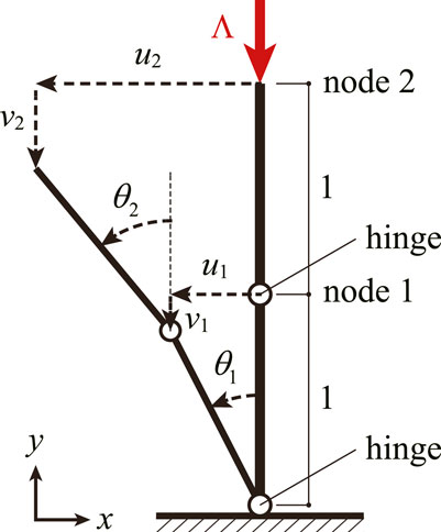
FIGURE 4. Configuration and variables of planar frame.

4.1.2 Stability of undeformed shape

In this section, the stability of the equilibrium state of the two-member frame shown in Figure 4 is evaluated by the eigenvalue analysis of the Hessian matrix of the augmented Lagrangian introduced in Section 3. Let W = 0 for the initial shape θ₁ = θ₂ = 0 of the frame. Assuming that W is fixed to W = 0, the Lagrange multiplier λ in the augmented Lagrangian is calculated as follows:

$\mathit{\lambda }=-\mathrm{\Lambda }{\left(\mathbf{\Gamma }{\left(\mathbf{0}\right)}^{+}\right)}^{\mathsf{T}}\mathbf{P}(30)$

where the superscript + denotes the Moore-Penrose generalized inverse. If λ is determined from Eq. 30, it satisfies the stationary condition ∇_WL_s (0, λ) = 0 for any Λ, i.e., the frame is in the equilibrium state for any Λ at W = 0. Therefore, the critical load factors are investigated at W = 0 by successively increasing the load factor Λ. Since the penalty parameter s in the augmented Lagrangian can be any value large enough at the equilibrium point, it is fixed to s = 1 × 10⁶ in this section for simplicity.

Figure 5A shows the smallest and second smallest eigenvalues of the Hessian matrix ${\nabla }_{\text{W}}^2{L}_s(\mathbf{0},\mathit{\lambda })$ when the load factor Λ is sequentially increased from 0 to 3. As shown in the figure, an eigenvalue becomes zero when Λ ≃Λ_cr1, Λ_cr2. The load factors at which an eigenvalue of the Hessian matrix of the augmented Lagrangian becomes zero coincide with the critical load factors at the undeformed equilibrium state obtained in Section 4.1.1. In addition, Figure 5B shows the critical eigenmodes. The values of θ₁ and θ₂ calculated from the eigenmodes are also shown. It can easily be confirmed that the eigenmodes ${(0.224,0.362)}^{\mathsf{T}}$ and ${(0.348,-0.215)}^{\mathsf{T}}$ obtained from ${\nabla }_{\text{W}}^2{L}_s(\mathbf{0},\mathit{\lambda })$ are identical (proportional) to x_cr1 and x_cr2 in Eq. 29, respectively, obtained analytically. From the above results, it is expected that the stability of the equilibrium state can be determined from the eigenvalues of the Hessian matrix of the augmented Lagrangian.

FIGURE 5

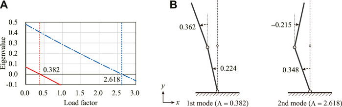
FIGURE 5. Eigenvalues of the Hessian matrix and the critical eigenmodes (A) Transition of the smallest and second smallest eigenvalues. (B) Critical eigenmodes at W = 0.

4.2 Waterbomb cell (1)

4.2.1 Stability of fully developed shape

Equilibrium path of the waterbomb cell shown in Figure 6 is investigated. The number of nodes, members, and hinges of the frame model are n_N = 22, n_M = 22, and n_H = 6, respectively. Hence, the number of components of the generalized displacement vector and the incompatibility vector are n_D = 264 and n_C = 264, respectively. As shown in Figure 6, the nodal loads are applied in the positive x-direction, and the boundary conditions are assigned to constrain the rigid-body motion of the model. The rotational stiffness of each spring installed in the hinge is determined to be proportional to the length of the corresponding crease line; 1 for a crease line of length 5 and $\sqrt{2}$ for a crease line of length $5\sqrt{2}$. Let W = 0 be a perfectly flat and developed state in which all nodes of the frame model lie on the xy-plane. The degrees of kinematic and static indeterminacy calculated from the rank of the compatibility matrix are both 4 atW = 0. Since the equilibrium state can be realized for any Λ at W = 0, the critical load factors are investigated at W = 0 by increasing the load factor and evaluating the eigenvalues of the Hessian matrix ${\nabla }_{\text{W}}^2{L}_s(\mathbf{0},\mathit{\lambda })$. As in Section 4.1.2, the Lagrange multiplier for each load factor is obtained from Eq. 30, and the penalty parameter is fixed at s = 1 × 10⁶.

FIGURE 6

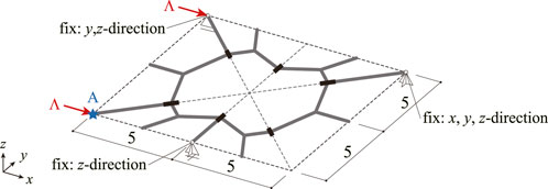
FIGURE 6. Configuration of analysis model, load, and boundary conditions; The frame model is represented by bold lines, and the edges of waterbomb cell are represented by dotted lines.

When the load factor Λ is increased from 0 to 5, the four smallest eigenvalues of ${\nabla }_{\text{W}}^2{L}_s(\mathbf{0},\mathit{\lambda })$ change as shown in Figure 7A. The fifth smallest eigenvalue is about 10000 times larger than the fourth smallest one. Three critical load factors are obtained as Λ_cr1 ≃ 0.280, Λ_cr2 ≃ 0.788, and Λ_cr3 ≃ 3.750, respectively. The critical eigenmodes at Λ = Λ_cr1, Λ_cr2, Λ_cr3 are shown in Figures 7B–D. Note that the number of critical load factors is equal to the degrees of kinematic indeterminacy at the folded state to be investigated in Section 4.2.2. The obtained critical points are the symmetric bifurcation points; i.e., denoting a critical eigenmode as W_cr, L_s (W_cr, λ) = L_s (−W_cr, λ) holds.

FIGURE 7

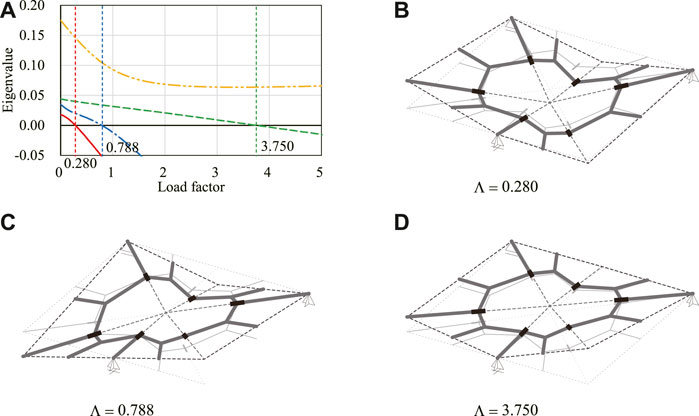
FIGURE 7. Eigenvalues and critical eigenmodes. (A) Smallest to the fourth smallest eigenvalues. (B) First critical eigenmode. (C) Second critical eigenmode. (D) Third critical eigenmode.

4.2.2 Equilibrium path analysis with initial imperfection

The equilibrium path analysis is carried out for the initial shape with the imperfection assigned by scaling each eigenmode shown in Figure 7. The three scales of imperfection modes are assigned and each analysis starts from W = W₀ so that the maximum nodal translation is w = 0.05, 0.1, 0.5, respectively. The maximum absolute value among the components of C(W₀) is about 1.07 × 10^–2 which corresponds to the component of the translational incompatibility vector and is about 1/1000 of the span of the model. To regard the rotation angles of the springs at W = W₀ as the undeformed state $\mathit{\phi }-\tilde{\mathit{\phi }}=\mathbf{0}$, the rotation angles of the hinges at W₀ multiplied by − 1 are assigned to $\tilde{\mathit{\phi }}$. When W = W₀, Λ = 0, and λ = 0, they approximately satisfy the stationary conditions of problem (21), and λ = 0 can be a good estimation of the multiplier corresponding to the stationary point of problem (15) at W = W₀ and Λ = 0. Therefore, the initial value of λ is given as λ = 0. The tolerance of the maximum error of C(W) is set as ϵ_tol = 1 × 10^–8. In this section, the penalty parameter s is updated automatically for the stability of the equilibrium path analysis. The initial increment of the load factor is dΛ₀ = 5.0, ×, 10^–3, and the update ratios of dΛ are a = 0.125 and b = 2.0. The maximum value of the load factor and the minimum value of the load factor increment are specified as Λ_max = 10.0 and dΛ_min = 1 × 10^–10, respectively. The reference displacement is the translation in the x-direction of node A at the lower left in Figure 6, with $W_i^{\text{max}}=10$ and $W_i^{\text{min}}=-1$. In order to investigate in detail the region where the reference displacement approaches $W_i^{\text{max}}$ or $W_i^{\text{min}}$, the increment of the load factor is adjusted appropriately to a value smaller than 5.0, ×, 10^–3.

Figure 8 shows the translation in the x-direction of node A for the analyses with nine different initial imperfections. Figure 9 shows the shape of the model on the equilibrium path with w = 0.05. The deformed shapes shown in Figures 9A,B are symmetrical with respect to the xy-plane. The degrees of kinematic and static indeterminacy are both 3 after the out-of-plane deformation occurs. The displacement progresses significantly in both cases around the first critical load factor Λ_cr1 ≃ 0.280. As shown in Figure 8, when the initial imperfection based on the first eigenmode is applied, the displacement progresses gradually before the load factor reaches the first critical load factor. On the other hand, when the initial imperfection based on the second or third eigenmode is applied, the displacement hardly progresses until the load factor exceeds the critical load factor. The deformed shapes at the end of the analysis are similar for all examples except for the symmetry about the xy-plane. The reason for the similarity of the final shapes is that the deformation occurs before the load factor reaches the second and third critical load factors since the critical load factors are isolated from each other. The equilibrium paths approximately converge to the deformation in the direction of the first eigenmode, i.e., the bifurcation path corresponding to the first critical point. The load factor is less than the second and third critical load factors even at the end of the equilibrium path analysis. The smallest eigenvalue of the Hessian matrix ${\nabla }_{\text{W}}^2{L}_s(\mathbf{W},\mathit{\lambda })$ on each equilibrium path is shown in Figure 10. The minimum value of the eigenvalue on each equilibrium path is also plotted in Figure 10 by × mark. The overall trend is that the eigenvalues have minima near the first critical load factor. It corresponds to the drastic increase of the deformation around the first critical load factor. The eigenvalues with the initial imperfection corresponding to the second and third critical eigenmodes oscillate in the range where the load factor is less than the first critical load factor. These oscillations are caused by the oscillations of the penalty parameters, and the drastic change of the penalty parameter in the range Λ < Λ_cr1 indicates the instability of finding the equilibrium point. It is reasonable that the equilibrium point with a small imperfection in the shape of the second or third eigenmode is difficult to find.

FIGURE 8

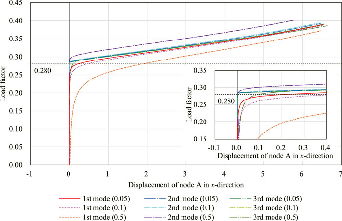
FIGURE 8. Displacement of node A in the x-direction with three different initial imperfection modes with three different magnitudes, respectively.

FIGURE 9

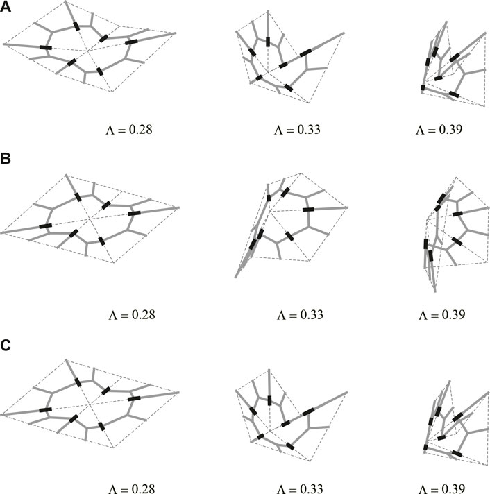
FIGURE 9. Deformed shapes with w = 0.05. (A) Imperfection corresponding to the first critical eigenmode. (B) Imperfection corresponding to the second critical eigenmode. (C) Imperfection corresponding to the third critical eigenmode.

FIGURE 10

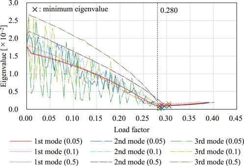
FIGURE 10. Transition of the smallest eigenvalue for each initial imperfection mode.

4.3 Waterbomb cell (2)

4.3.1 Stability of fully developed shape

Equilibrium path of the waterbomb cell shown in Figure 11 is investigated. The loading and boundary conditions are different from the previous example. This way, we can generate various deformation patterns of the waterbomb cell. The number of nodes, members, and hinges of the frame model are n_N = 22, n_M = 22, and n_H = 6, respectively. Hence, the number of components of the generalized displacement vector and the incompatibility vector are n_D = 264 and n_C = 264, respectively. The degrees of kinematic and static indeterminacy are both 4 at W = 0. As in Section 4.2, the critical load factor at W = 0 is obtained by evaluating the eigenvalues of the Hessian matrix ${\nabla }_{\text{W}}^2{L}_s(\mathbf{0},\mathit{\lambda })$ of the augmented Lagrangian by successively increasing the load factor. The penalty parameter is fixed at s = 1 × 10⁶.

FIGURE 11

FIGURE 11. Configuration of analysis model, load, and boundary conditions.

Figure 12A shows the change of the four smallest eigenvalues of ${\nabla }_{\text{W}}^2{L}_s(\mathbf{0},\mathit{\lambda })$ when the load factor Λ is increased from 0 to 5. The fifth smallest eigenvalue is more than 10000 times larger than the fourth smallest one. Three critical load factors are obtained as Λ_cr1 ≃ 1.137, Λ_cr2 ≃ 2.704, and Λ_cr3 ≃ 2.909, respectively. Figures 12B–D show the critical eigenmodes at Λ = Λ_cr1, Λ_cr2, Λ_cr3. The obtained critical points are the symmetric bifurcation points.

FIGURE 12

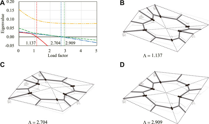
FIGURE 12. Eigenvalues and critical eigenmodes. (A) Smallest to the fourth smallest eigenvalues. (B) First critical eigenmode. (C) Second critical eigenmode. (D) Third critical eigenmode.

4.3.2 Equilibrium path analysis with initial imperfection

Equilibrium path analysis is performed for the shape with initial imperfection based on the eigenmodes shown in Figure 12. The conditions for analysis are the same as those in Section 4.2, except for dΛ₀ and Λ_max, which are set as dΛ₀ = 0.01 and Λ_max = 15.0, respectively. The maximum absolute value among the components of C(W₀) is about 1.66 × 10^–2 which corresponds to the component of the translational incompatibility vector and is about 1/600 of the span of the model. The displacement in the x-direction of node A in Figure 11 is used as the reference displacement.

Figure 13 shows the relation between the displacement at node A and the load factor. The shapes of the model on the equilibrium path with each initial imperfection mode with w = 0.05 are shown in Figure 14. The deformed shapes shown in Figures 14A,B are symmetric with respect to the xy-plane. The degrees of kinematic and static indeterminacy are both 3 after the out-of-plane deformation occurs. As shown in the figure, the displacement progresses significantly around the first critical load factor Λ_cr1 ≃ 1.137 in both cases of initial imperfection. As in Section 4.2.2, the final shapes of the analysis are almost identical since the critical load factors are isolated. The smallest eigenvalue of ${\nabla }_{\text{W}}^2{L}_s(\mathbf{W},\mathit{\lambda })$ on each equilibrium path is shown in Figure 15. Similarly to the results in Section 4.2.2, the overall trend is that the eigenvalues have minima near the first critical load factor. The minimum values of the eigenvalues on the equilibrium paths are plotted in Figure 15 by × marks. In contrast to the example in Section 4.2.2, the load factor exceeds the second and third critical load factors at the final stage of analysis. However, when Λ exceeds Λ_cr1, a finite deformation occurs and all eigenvalues are positive for each equilibrium path as shown in Figures 13, 15. Therefore, the equilibrium state is always stable after the load factor exceeds the first critical load factor.

FIGURE 13

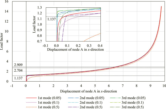
FIGURE 13. Displacement of node A in the x-direction with three different initial imperfection modes with three different magnitudes, respectively.

FIGURE 14

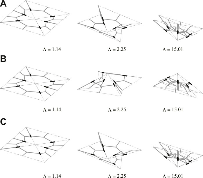
FIGURE 14. Deformed shapes with w = 0.05. (A) Imperfection corresponding to the first critical eigenmode. (B) Imperfection corresponding to the second critical eigenmode. (C) Imperfection corresponding to the third critical eigenmode.

FIGURE 15

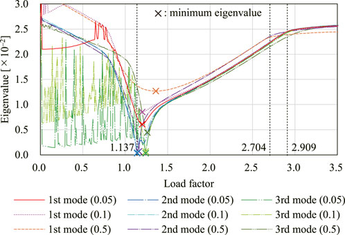
FIGURE 15. Transition of the smallest eigenvalue for each initial imperfection mode.

5 Conclusion

This paper has presented a method of equilibrium path and stability analysis of a rigid origami represented by a frame model. Rotational springs are installed into hinges and nodal loads are applied to a frame model. The rotational springs allow the equilibrium path to be uniquely determined locally except at the critical points. An equilibrium state is achieved for a specified load factor by minimizing the total potential energy of the frame under the compatibility conditions so that the displacements of nodes and members and the rotations of hinges are compatible. The energy minimization problem is solved by the augmented Lagrangian method. An equilibrium path is obtained by successively solving the energy minimization problem while increasing the load factor. Stability of an equilibrium point is evaluated by the eigenvalues of the Hessian matrix of the augmented Lagrangian. If the Hessian matrix is positive definite at an equilibrium point, the total potential energy is local minimum and the equilibrium state is stable. Conversely, if the Hessian matrix has a zero eigenvalue, the equilibrium point is a candidate for a bifurcation or a limit point.

The proposed method was first applied to a planar frame consisting of two members whose analytical solution can be easily obtained. It has been confirmed that the analytical solution and the result of the stability analysis proposed in this paper agree with good accuracy, i.e., critical load factors that may cause instability in the equilibrium can be determined by the proposed method. After verifying the validity of the proposed method, the method was applied to fully developed flat waterbomb cells with two different loads and boundary conditions. As shown in the numerical examples, various equilibrium paths can be obtained from the same crease pattern by changing the loads and boundary conditions. At the flat state, three critical load factors are found in each example. The number of critical load factors of each example is equal to the degrees of kinematic indeterminacy at the folded state, not at the flat state. The initial imperfection based on a critical mode is assigned in the equilibrium path analysis to avoid the multiple bifurcation at the flat state and to investigate the impact of the initial imperfection on the equilibrium path. The out-of-plane deformation drastically progresses after the load factor exceeds the first critical load factor. Although three different initial imperfection modes are assigned with three different magnitudes, respectively, similar final shapes are obtained because the critical points are isolated and the equilibrium paths converge to the bifurcation path of the first critical point. These results suggest that waterbomb cells can be used to realize a structure that can be easily and safely deployed.

Since the proposed method supports only the load increment method at present, it is insufficient as a method for equilibrium path analysis of mechanisms with strong nonlinearity. It is expected in future work that the proposed method is extended to include the incremental displacement method and the arc length method. In addition, the augmented Lagrangian is minimized using BFGS in this study, and the computation cost is proportional to the square of the number of faces since the number of variables in the optimization problem is proportional to the number of faces of a rigid origami. This leads to a substantial computational cost for the analysis of large-scale origami. Therefore, the number of variables should be reduced by eliminating the dependent variables for the analysis of large-scale origami.

Data availability statement

The raw data supporting the conclusions of this article will be made available by the authors, without undue reservation.

Author contributions

KH and MO contributed to conception and design of the study. KH performed the analysis and wrote the first draft of the manuscript. All authors contributed to manuscript revision, read, and approved the submitted version.

Funding

This work is supported by JSPS KAKENHI Grant Number JP20J21650, JP19K04714 and JST CREST Grant Number JPMJCR1911.

Acknowledgments

We acknowledge Akito Adachi at Kyoto University for his insightful comments and suggestions.

Conflict of interest

The authors declare that the research was conducted in the absence of any commercial or financial relationships that could be construed as a potential conflict of interest.

Publisher’s note

All claims expressed in this article are solely those of the authors and do not necessarily represent those of their affiliated organizations, or those of the publisher, the editors and the reviewers. Any product that may be evaluated in this article, or claim that may be made by its manufacturer, is not guaranteed or endorsed by the publisher.

Supplementary material

The Supplementary Material for this article can be found online at: https://www.frontiersin.org/articles/10.3389/fbuil.2022.995710/full#supplementary-material

Footnotes

¹http://www.tsg.ne.jp/TT/software/.

²https://paulino.ce.gatech.edu/software.html.

³https://origamisimulator.org/.

References

Bažant, Z. P., and Cedolin, L. (2010). Stability of structures: Elastic, inelastic, fracture and damage theories. World Scientific Publishing Co. Pte. Ltd.

Google Scholar

Belke, C. H., and Paik, J. (2017). Mori: A modular origami robot. Ieee. ASME. Trans. Mechatron. 22, 2153–2164. doi:10.1109/TMECH.2017.2697310

CrossRef Full Text | Google Scholar

Birgin, E. G., and Martínez, J. M. (2012). Augmented Lagrangian method with nonmonotone penalty parameters for constrained optimization. Comput. Optim. Appl. 51, 941–965. doi:10.1007/s10589-011-9396-0

CrossRef Full Text | Google Scholar

Chen, B. G., and Santangelo, C. D. (2018). Branches of triangulated origami near the unfolded state. Phys. Rev. X 8, 011034. doi:10.1103/PhysRevX.8.011034

CrossRef Full Text | Google Scholar

Chen, Y., Fan, L., Bai, Y., Feng, J., and Sareh, P. (2020). Assigning mountain-valley fold lines of flat-foldable origami patterns based on graph theory and mixed-integer linear programming. Comput. Struct. 239, 106328. doi:10.1016/j.compstruc.2020.106328

CrossRef Full Text | Google Scholar

Demaine, E. D., Demaine, M. D., Huffman, D. A., Hull, T. C., Koschitz, D., and Tachi, T. (2016). “Zero-area reciprocal diagram of origami,” in Proceedings of the IASS Annual Symposium 2016, Tokyo, Japan.

Google Scholar

Filipov, E. T., Liu, K., Tachi, T., Schenk, M., and Paulino, G. H. (2017). Bar and hinge models for scalable analysis of origami. Int. J. Solids Struct. 124, 26–45. doi:10.1016/j.ijsolstr.2017.05.028

CrossRef Full Text | Google Scholar

Forst, W., and Hoffmann, D. (2010). Optimization: Theory and practice. Springer.

Google Scholar

Géradin, M., and Cardona, A. (2007). Flexible multibody dynamics: A finite element approach. Hoboken, NJ, United States: Wiley.

Google Scholar

Ghassaei, A., Demaine, E. D., and Gershenfeld, N. (2018). “Fast, interactive origami simulation using GPU computation,” in Proceedings of the 7th international meeting of origami science, mathematics, and education (Origami7). Editors R. J. Lang, M. Bolitho, and Z. You. (St Albans, United Kingdom: Tarquin), 1151–1156.

Google Scholar

Gillman, A., Fuchi, K., and Buskohl, P. R. (2018). Truss-based nonlinear mechanical analysis for origami structures exhibiting bifurcation and limit point instabilities. Int. J. Solids Struct. 147, 80–93. doi:10.1016/j.ijsolstr.2018.05.011

CrossRef Full Text | Google Scholar

Hayakawa, K., and Ohsaki, M. (2021). Form generation of rigid origami for approximation of a curved surface based on mechanical property of partially rigid frames. Int. J. Solids Struct. 216, 182–199. doi:10.1016/j.ijsolstr.2020.12.007

CrossRef Full Text | Google Scholar

Hayakawa, K., and Ohsaki, M. (2019a). Form generation of rigid-foldable origami structure using frame model. J. Environ. Eng. New. York. 84, 597–605. (in Japanese). doi:10.3130/aije.84.597

CrossRef Full Text | Google Scholar

Hayakawa, K., and Ohsaki, M. (2019b). “Frame model for analysis and form generation of rigid origami for deployable roof structure,” in Proceedings of the IASS Annual Symposium 2019, Barcelona, Spain, 1080–1087.

Google Scholar

He, Z., and Guest, S. D. (2022). On rigid origami III: Local rigidity analysis. Proc. Math. Phys. Eng. Sci. 478, 20210589. doi:10.1098/rspa.2021.0589

PubMed Abstract | CrossRef Full Text | Google Scholar

Hestenes, M. R. (1969). Multiplier and gradient methods. J. Optim. Theory Appl. 4, 303–320. doi:10.1007/BF00927673

CrossRef Full Text | Google Scholar

Izmailov, A. F., and Solodov, M. V. (2015). Critical Lagrange multipliers: What we currently know about them, how they spoil our lives, and what we can do about it. TOP 23, 1–26. doi:10.1007/s11750-015-0372-1

CrossRef Full Text | Google Scholar

Katoh, N., and Tanigawa, S. (2011). A proof of the molecular conjecture. Discrete Comput. Geom. 45, 647–700. doi:10.1007/s00454-011-9348-6

CrossRef Full Text | Google Scholar

Kawaguchi, M. (1991). Design problems of long span spatial structures. Eng. Struct. 13, 144–163. doi:10.1016/0141-0296(91)90048-H

CrossRef Full Text | Google Scholar

Kuribayashi, K., Tsuchiya, K., You, Z., Tomus, D., Umemoto, M., Ito, T., et al. (2006). Self-deployable origami stent grafts as a biomedical application of ni-rich tini shape memory alloy foil. Mater. Sci. Eng. A 419, 131–137. doi:10.1016/j.msea.2005.12.016

CrossRef Full Text | Google Scholar

Lee, T.-U., and Gattas, J. M. (2016). Geometric design and construction of structurally stabilized accordion shelters. J. Mech. Robot. 8, 031009. doi:10.1115/1.4032441

CrossRef Full Text | Google Scholar

Li, Y. (2020). Motion paths finding for multi-degree-of-freedom mechanisms. Int. J. Mech. Sci. 185, 105709. doi:10.1016/j.ijmecsci.2020.105709

CrossRef Full Text | Google Scholar

Liu, K., and Paulino, G. H. (2018). “Highly efficient nonlinear structural analysis of origami assemblages using the merlin2 software,” in Proceedings of the 7th international meeting of origami science, mathematics, and education (Origami7). Editors R. J. Lang, M. Bolitho, and Z. You. (St Albans, United Kingdom: Tarquin), 1197–1182.

Google Scholar

Ma, J., and You, Z. (2013). Energy absorption of thin-walled square tubes with a prefolded origami pattern-part I: Geometry and numerical simulation. J. Appl. Mech. 81, 011003. doi:10.1115/1.4024405

CrossRef Full Text | Google Scholar

Meloni, M., Cai, J., Zhang, Q., Lee, D. S., Li, M., Ma, R., et al. (2021). Engineering origami: A comprehensive review of recent applications, design methods, and tools. Adv. Sci. 8, 2000636. doi:10.1002/advs.202000636

CrossRef Full Text | Google Scholar

Miura, K., and Pellegrino, S. (2020). Forms and concepts for lightweight structures. Cambridge, UK: Cambridge University Press.

Google Scholar

Morales, J. L., and Nocedal, J. (2011). Remark on ”algorithm 778: L-BFGS-B: Fortran subroutines for large-scale bound constrained optimization. ACM Trans. Math. Softw. 38, 1–4. doi:10.1145/2049662.2049669

CrossRef Full Text | Google Scholar

Ohsaki, M., and Ikeda, K. (2006). Imperfection sensitivity analysis of hill-top branching with many symmetric bifurcation points. Int. J. Solids Struct. 43, 4704–4719. doi:10.1016/j.ijsolstr.2005.06.036

CrossRef Full Text | Google Scholar

Ohsaki, M., and Ikeda, K. (2007). Stability and optimization of structures: Generalized sensitivity analysis. New York, United States: Springer.

Google Scholar

Ohsaki, M., Tsuda, S., and Miyazu, Y. (2016). Design of linkage mechanisms of partially rigid frames using limit analysis with quadratic yield functions. Int. J. Solids Struct. 88-89, 68–78. doi:10.1016/j.ijsolstr.2016.03.023

CrossRef Full Text | Google Scholar

Reis, P. M., Jiménez, F. L., and Marthelot, J. (2015). Transforming architectures inspired by origami. Proc. Natl. Acad. Sci. U. S. A. 112, 12234–12235. doi:10.1073/pnas.1516974112

PubMed Abstract | CrossRef Full Text | Google Scholar

Saito, K., Tsukahara, A., and Okabe, Y. (2015). New deployable structures based on an elastic origami model. J. Mech. Des. N. Y. 137, 021402. doi:10.1115/1.4029228

CrossRef Full Text | Google Scholar

Salerno, G. (1992). How to recognize the order of infinitesimal mechanisms: A numerical approach. Int. J. Numer. Methods Eng. 35, 1351–1395. doi:10.1002/nme.1620350702

CrossRef Full Text | Google Scholar

Schenk, M., and Guest, S. D. (2011). “Origami folding: A structural engineering approach,” in Proceedings of the 5th international meeting of origami science, mathematics, and education (Origami5). Editors P. Wang-Iverson, R. J. Lang, and M. Yim (Boca Raton, FL, United States: CRC Press), 291–303.

Google Scholar

Shende, S., Gillman, A., Yoo, D., Buskoh, P., and Vemaganti, K. (2021). Bayesian topology optimization for efficient design of origami folding structures. Struct. Multidiscipl. Optim. 63, 1907–1926. doi:10.1007/s00158-020-02787-x

CrossRef Full Text | Google Scholar

Silverberg, J. L., Evans, A. A., McLeod, L., Hayward, R. C., Hull, T., Santangelo, C. D., et al. (2014). Using origami design principles to fold reprogrammable mechanical metamaterials. Science 345, 647–650. doi:10.1126/science.1252876

PubMed Abstract | CrossRef Full Text | Google Scholar

Tachi, T. (2012). Design of infinitesimally and finitely flexible origami based on reciprocal figures. J. Geometry Graph. 16, 223–234.

Google Scholar

Tachi, T. (2010). “Geometric considerations for the design of rigid origami structures,” in Proceedings of the IASS Annual Symposium 2010, Shanghai, China, 8–12.

Google Scholar

Tachi, T., and Hull, T. C. (2017). Self-foldability of rigid origami. J. Mech. Robot. 9 (1), 021008. doi:10.1115/1.4035558

CrossRef Full Text | Google Scholar

Tachi, T. (2009). “Simulation of rigid origami,” in Proceedings of the 4th international meeting of origami science, mathematics, and education (Origami4). Editor R. J. Lang (Natick, MA, United States: AK Peters), 175–187.

Google Scholar

Thompson, J. M. T., and Hunt, G. W. (1973). A general theory of elastic stability. Wiley.

Google Scholar

Tsuda, S., Ohsaki, M., Kikugawa, S., and Kanno, Y. (2013). Analysis of stability and mechanism of frames with partially rigid connections. Nihon. Kenchiku. Gakkai. Kozokei. Ronbunshu. 78, 791–798. (in Japanese). doi:10.3130/aijs.78.791

CrossRef Full Text | Google Scholar

Watada, R., and Ohsaki, M. (2018). Series expansion method for determination of order of 3-dimensional bar-joint mechanism with arbitrarily inclined hinges. Int. J. Solids Struct. 141-142, 78–85. doi:10.1016/j.ijsolstr.2018.02.012

CrossRef Full Text | Google Scholar

Watanabe, N. (2018). Foldable condition in a singular state of a rigid origami model. Trans. Jpn. Soc. Industrial Appl. Math. 28, 54–71. (in Japanese). doi:10.11540/jsiamt.28.1_54

CrossRef Full Text | Google Scholar

Zhang, T., Kawaguchi, K., and Wu, M. (2018). A folding analysis method for origami based on the frame with kinematic indeterminacy. Int. J. Mech. Sci. 146-147, 234–248. doi:10.1016/j.ijmecsci.2018.07.036

CrossRef Full Text | Google Scholar

Zirbel, S. A., Lang, R. J., Thomson, M. W., Sigel, D. A., Walkemeyer, P. E., Trease, B. P., et al. (2013). Accommodating thickness in origami-based deployable Arrays1. J. Mech. Des. N. Y. 135, 111005. doi:10.1115/1.4025372

CrossRef Full Text | Google Scholar