Wave Attenuation by Vegetation: Model Implementation and Validation Study

Wave–vegetation interaction is implemented in the WAVEWATCH III (WW3) model. The vegetation sink term followed the early formulations of Dalrymple et al. (Journal of Waterway, Port, Coastal, and Ocean Engineering, 1984, 110, 67–79), which focused on monochromatic waves and vegetation approximated as an array of rigid, vertical cylinders, and was later expanded by Mendez and Losada (Coastal Engineering, 2004, 51, 103–118) for random wave transformations over mildly sloping vegetation fields under breaking and nonbreaking conditions assuming a Rayleigh distribution of wave heights. First, validation is carried out for 63 laboratory cases (Anderson and Smith, 2014) with homogeneous vegetation fields for single and double-peak wave spectra. Then, a field case application is conducted to assess the wave attenuation in a wetland environment with spatially variable vegetation fields during stormy conditions. The case study uses data collected at the Magothy Bay located in the Chesapeake Bay, United States, during Hurricanes Jose and Maria in 2017. The domain decomposition parallelization and the implicit scheme have been used for the simulations to efficiently resolve complex shorelines and high-gradient wave zones, incorporating dominant physics in the complicated coastal zone, including wave breaking, wave–current interaction, bottom friction and scattering, wave–vegetation interaction, and nonlinearity (Abdolali et al., 2020). The lab validation and field application demonstrate that WW3 is an effective tool for evaluating the capacity of wetland natural or nature-based features to attenuate wave energy to achieve coastal flood risk reduction.

1 Introduction

Wetlands are key natural and nature-based features used to dissipate wave energy and reduce flood risk. Historically, the operational practice to account for wave energy reduction due to wetland vegetation was through bottom friction sink terms implemented in nearshore wave models. The formulations most often applied use Manning’s roughness coefficients n, which traditionally described bottom roughness in uniform flows for open channels and floodplains (Chow, 1959). These Manning’s coefficients n account for spatial variations tied to local terrain and roughness, and many numerical studies, particularly those coupling phase-averaged wave models to hydrodynamic models such as the ADvanced CIRCulation model (ADCIRC), select Manning’s n based on land-cover databases and standard hydraulic literature (Dietrich et al., 2011; Bender et al., 2013; Hope et al., 2013; Lawler et al., 2016; Bryant and Jensen, 2017). Controlled laboratory experiments continue to highlight the complexity of wave–vegetation interactions, most notably the effect of vegetation properties such as rigidity, height, density, and diameter on wave attenuation (Anderson and Smith, 2014; Ozeren et al., 2014; Luhar et al., 2017; Jacobsen et al., 2019; Phan et al., 2019; van Veelen et al., 2020). These studies suggest there are key physics that Manning’s n does not properly represent, such as the drag force exerted on the water column due to temporally and spatially varying immersed vegetation. These potential shortfalls of Manning’s n led to the derivation and subsequent implementation of vegetation-dissipation sink terms in widely used nearshore wave models, such as WWM-III (Roland, 2008), SWAN (Suzuki et al., 2012), STWAVE (Anderson and Smith, 2015), and XBEACH (Van Rooijen et al., 2015). These vegetation-dissipation sink terms are a function of the local hydrodynamic conditions and account directly for measurable vegetation characteristics. Both Smith et al. (2016) and Baron-Hyppolite et al. (2019) reported an underestimation of wave dissipation using enhanced Manning’s n to represent vegetation compared to vegetation-dissipation formulations that explicitly account for plant properties.

The fundamental formulation for wave dissipation through vegetation was derived by Dalrymple et al. (1984) for monochromatic waves using the conservation of energy flux equation, where the horizontal force F_x acting on the vegetation per unit volume is expressed in terms of a Morison-type equation neglecting swaying motion and inertial force:

$F_x=\frac{1}{2}\rho C_d{b}_{\nu }Nu|u|(1)$

where ρ is water density, C_d is the depth-averaged bulk drag coefficient, b_v is stem diameter, N is plant density (stems/m²), and u is horizontal velocity due to wave motion.

Although plant motion is neglected, Eq. 1 may still be applied to swaying plants because the bulk drag coefficient C_d accounts for our ignorance of plant motion, interactions between stems, and other unresolved processes. Indeed, Mendez et al. (1999) stated that using the relative velocity between the fluid and plant required a higher value of C_d to obtain the same amount of attenuation. Mendez and Losada (2004) expanded upon Dalrymple et al. (1984) and derived an analytical solution for random wave transformations over mildly sloped vegetation fields under breaking and nonbreaking conditions by assuming a Rayleigh distribution of wave heights. The modification by Mendez and Losada (2004) is incorporated into several phase-averaged nearshore wave models similar to Suzuki et al. (2012), with verification largely focused on laboratory studies, albeit field applications are now gaining traction (Garzon et al., 2019). As an alternative to field surveys to collect vegetation properties, Figueroa-Alfaro et al. (2022) proposed a modified parameterization using a leaf area index-based measurement that can be readily derived from satellite imagery, but its application is limited to emergent vegetation. While these developments are advancing wave–vegetation modeling, continued research into the drag coefficient C_d, which directly affects the dissipation rate, is critical given the growing concerns regarding its assumptions and derivations (Tempest et al., 2015).

This study is arranged as follows: a summary of the implementation of Mendez and Losada (2004) in WAVEWATCH III (WW3) is presented in Section 2; Section 3 provides a brief overview of the validation studies using laboratory data of homogeneous vegetation fields and field case application with observations in Virginia during Hurricanes Jose and Maria in 2017; and concluding remarks are provided in Section 4.

2 Formulation

In spectral wave models such as WW3, the waves are defined in terms of wave action density spectrum N (σ, θ) as a function of angular wave frequency and wave direction:

$\frac{\partial }{\partial t}N+{\nabla }_x\left(c_g+\mathbf{U}\right)N+\frac{\partial }{\partial \sigma }{c}_{\sigma }N+\frac{\partial }{\partial \theta }{c}_{\theta }N=\frac{S}{\sigma }(2)$

where N (k, θ) is the wave action density spectrum related to the wave energy density spectrum F (k, θ), where N (k, θ) = F (k, θ)/σ and c_g, U, c_σ, and c_θ are the group velocity, the current velocity depth-time averaged over the scales of individual waves, propagation velocity in frequency σ, and direction θ spaces, respectively.

The terms on the left-hand side of Equation 2 represent wave action density change in time, propagation in geographical space, shifting of the relative frequency due to changes in current and depth, and depth and current-induced refraction, respectively.

The energy density source term S is placed on the right-hand side of Eq. 2 and accounts for generation (i.e., by wind), dissipation (i.e., whitecapping, bottom friction, depth induced breaking), and nonlinear wave–wave interaction.

Without vegetation, wave energy flux remains constant if no energy is lost or gained. In the presence of vegetation, the wave energy flux, following Dalrymple et al. (1984), Kobayashi et al. (1993)m and Mendez and Losada (2004) becomes

$\frac{\partial F}{\partial x}=-{ϵ}_{\nu }\to \frac{\partial }{\partial x}\left[E.c_g\right]=-{ϵ}_{\nu }(3)$

where wave energy is defined as

$E=\frac{1}{8}\rho g{H}^2(4)$

and ϵ_ν is a function of the drag force F_x (Equation 1) integrated over the height of the vegetation

${ϵ}_{\nu }=\overline{{\int }_{-h}^{-h+\alpha h}{F}_{x}udz}(5)$

Assuming linear wave theory is valid to calculate u, the horizontal velocity due to wave motion, the mean rate of energy dissipation per unit horizontal area ϵ_ν due to wave damping by vegetation becomes

${ϵ}_{\nu }=\frac{1}{2\sqrt{\pi }}\rho C_d{b}_{\nu }N{\left(\frac{kg}{2\sigma }\right)}^3\frac{{\sinh }^3\left(k\alpha h\right)+3\sinh \left(k\alpha h\right)}{3k{\cosh }^3\left(kh\right)}{H}_{rms}^3(6)$

where k is wave number, α is the ratio of plant height l_s to water depth h (L_s/h), and H_rms is root mean square wave height.

Combining Eqs (3)–(6),

$\frac{\partial H_{rms}^2}{\partial x}=\frac{-{ϵ}_{\nu }}{\frac{1}{8}\rho g{c}_g}=\frac{2}{3\sqrt{\pi }}{C}_d{b}_{\nu }Nk\frac{{\sinh }^3\left(k\alpha h\right)+3\sinh \left(k\alpha h\right)}{\left[\sinh \left(2kh\right)+2kh\right]\sinh \left(kh\right)}{H}_{rms}^3(7)$

A spectral version implemented in WW3 is divided by − ρg and written in a spectral/directional form:

$S_{veg}\left(\sigma ,\theta \right)=\frac{D_{tot}}{E_{tot}}E\left(\sigma ,\theta \right)(8)$

$D_{tot}=-\frac{1}{2g\sqrt{\pi }}{C}_d{b}_{\nu }N{\left(\frac{\bar{k}g}{2\bar{\sigma }}\right)}^3\frac{{\sinh }^3\left(\bar{k}\alpha h\right)+3\sinh \left(\bar{k}\alpha h\right)}{3\bar{k}{\cosh }^3\left(\bar{k}h\right)}{H}_{rms}^3(9)$

where the mean frequency $\bar{\sigma }$, mean wave number $\bar{k}$, and total wave energy E_tot are given by

$\bar{\sigma }={\left(\frac{1}{E_{tot}}{\int }_0^{2\pi }{\int }_0^{\infty }\frac{1}{\sigma }E\left(\sigma ,\theta \right)d\sigma d\theta \right)}^{-1}(10)$

$\bar{k}={\left(\frac{1}{E_{tot}}{\int }_0^{2\pi }{\int }_0^{\infty }\frac{1}{\sqrt{k}}E\left(\sigma ,\theta \right)d\sigma d\theta \right)}^{-2}(11)$

$E_{tot}={\int }_0^{2\pi }{\int }_0^{\infty }E\left(\sigma ,\theta \right)d\sigma d\theta (12)$

Finally, substituting $H_{rms}^2=8E_{tot}$, the wave–vegetation sink term becomes (Suzuki et al., 2012)

$S_{d,veg}=-\sqrt{\frac{2}{\pi }}{g}^2{C}_d{b}_{\nu }N{\left(\frac{\bar{k}}{\bar{\sigma }}\right)}^3\frac{{\sinh }^3\left(\bar{k}\alpha h\right)+3\sinh \left(\bar{k}\alpha h\right)}{3\bar{k}{\cosh }^3\left(\bar{k}h\right)}\sqrt{E_{tot}}E\left(\sigma ,\theta \right)(13)$

Although not currently in WW3, the spectral wave–vegetation sink term formulated by Suzuki et al. (2012) may consider different densities and stem widths between trunks and roots (i.e., mangrove trees) by considering layer schematization. Recent developments by Dalrymple et al. (1984) and Mendez and Losada (2004) include implementation into mild slope equation models (Tang et al., 2015) and the incorporation of wave–current interactions for both following and opposing currents (Losada et al., 2016).

3 Validation

After implementing the vegetation sink term in WW3, we verified for idealized laboratory experiments, consisting of 63 cases with homogeneous vegetation fields. Then, we progressed to the large-scale field test case for Hurricanes Jose and Maria (2017).

3.1 Laboratory Experiments (Anderson and Smith, 2014)

The Anderson and Smith (2014) experiments were performed at the U.S. Army Engineer Research and Development Center in Vicksburg, Mississippi, in a 63.4 m long, 1.5 m wide, and 1.5 m deep wave flume equipped with a piston-type wave-maker (Figure 1). A 9.8 m long vegetation zone, populated with idealized Spartina alterniflora vegetation, was located 29.3 m from the wave-maker. The idealized vegetation was constructed of b_v = 6.4 mm diameter and l_s = 41.5 cm tall flexible polyolefin tubing considering two stem densities of N = 200 and 400 stems/m² (corresponding to an element spacing of 7.1 and 5 cm, respectively). Given the inherent complexities live vegetation introduces to the laboratory, Anderson and Smith (2014) selected polyolefin tubing similar in dimension and rigidity to Spartina alterniflora measured along the Louisiana coast (Chatagnier, 2012) in order to best approximate biomechanical properties of the real vegetation. The water depths of the experiments were h = 30.5, 45.7, and 53.3 cm, simulating both submerged (l_s/h = 0.78, 0.91) and emergent (l_s/h = 1.0) conditions. The periods and significant wave heights for the the incident irregular waves with single- and double-peak periods vary between T_p = 1.25–2.25 s and H_m0 = 5–19.2 cm, respectively. Wave attenuation by the vegetation was assessed relative to a bare control run (no vegetation) for each wave condition. A summary of the wave conditions tested by Anderson and Smith (2014) for each vegetation density is provided in Table 1.

FIGURE 1

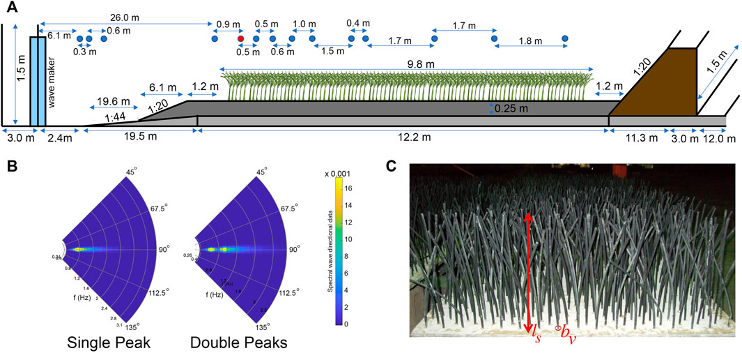
FIGURE 1. (A) Schematic view of Anderson and Smith (2014) wave flume. (B) Single-peak and double-peak spectral density data for boundary forcing at the wave-maker in the flume and numerical model (red dot in panel (a)). (C) Installed idealized vegetation (vegetation height l_s and vegetation thickness b_v).

TABLE 1

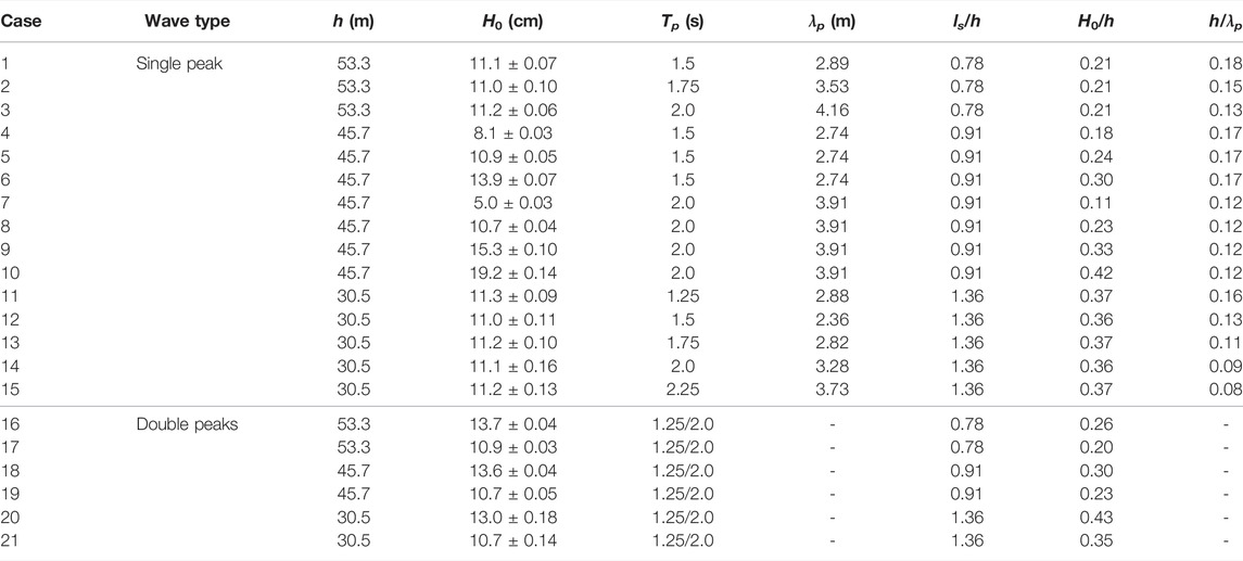
TABLE 1. Wave condition at the beginning of vegetation zone (5th gauge from wave-maker).

The bulk drag coefficient (C_d) is a function of wave parameters and vegetation species/characteristics. The relationship between C_d and flow parameters is given by

$C_d\left(Re\right)={\alpha }_1+{\left(\frac{{\alpha }_2}{Re}\right)}^{{\alpha }_3}(14)$

for flow characteristics defined by Reynolds number:

$Re=\frac{u_c{b}_v}{\nu }(15)$

where ν = 10^–6 m²/s is kinematic viscosity of water and u_c is the characteristic velocity acting on the plant. The characteristic velocity is defined here as the maximum horizontal velocity immediately in the front of the vegetation field as shown by red circle in Figure 1:

$u_{\mathit{max}}=\frac{\sigma a}{\tanh \left(kh\right)}(16)$

where H_s and T_p correspond to monochromatic wave train characteristics and the depth is z = h (1 − α). The Keulegan–Carpenter number is a dimensionless number that describes the relative importance of the drag force over inertia for a vertical obstacle in an oscillating flow:

$KC=\frac{u_{\mathit{max}}{T}_p}{b_{\nu }}(17)$

The relation between C_d and KC number is evaluated based on experiments.

Following Kobayashi et al. (1993) and Mendez and Losada (2004) and considering the correction due to the canopy submergence (Ls/h), the empirical relationship between C_d and the nondimensional numbers Q_Re and Q_KC is shown in Figure 2 and given by

$C_d\left(Q_{Re}\right)={\theta }_1+{\left(\frac{{\theta }_2}{Q_{Re}}\right)}^{{\theta }_3};C_d\left(Q_{KC}\right)={\lambda }_1+{\left(\frac{{\lambda }_2}{Q_{KC}}\right)}^{{\lambda }_3}(18)$

where [θ₁, θ₂, θ₃] = [ − 0.22, 765.11, 0.67], [λ₁, λ₂, λ₃] = [0.25, 24.87, 2.15], and

$Q_{Re}=\frac{Re}{{\left(l_s/h\right)}^{1.5}};Q_{KC}=\frac{KC}{{\left(l_s/h\right)}^{1.5}}(19)$

FIGURE 2

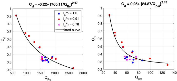
FIGURE 2. Bulk drag coefficient C_d as a function of (left) modified stem Reynolds number Q_Re and (right) modified Keulegan–Carpenter number Q_KC accounting for stem submergence ratio for Anderson and Smith (2014) dataset. Different symbols represent different values of l_s/h.

The results are shown in Figure 3 for two-single-peak (#6 and #12) and two-double-peak (#17 and #21) wave spectra. The spectra density observed at the 5th gauge in the flume and the corresponding forcing boundary condition at the WW3 wave-maker are shown in the upper panels. The time series of the significant wave heights extracted from the model (solid) is compared with the observations (dashed), shown in the lower panels for no vegetation (black), N = 200 (blue) and N = 400 stems/m² (black). The outputs of the model show a good agreement with the laboratory measurement for the wave attenuation due to wave–vegetation as a function of distance from the wave-maker.

FIGURE 3

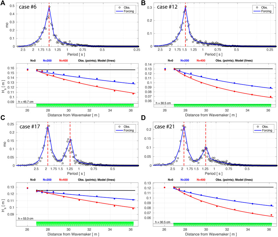
FIGURE 3. Upper panels) Spectral density for single-peak (A,B) and double-peak (C,D) waves at the 5^th gauge in the flume (black circles) and boundary forcing in the WW3 model (solid blue). The dashed red lines show the peak(s). (Lower panels) Significant wave height observed in the lab (circles) and from the WW3 model (solid) for no vegetation (black), N =200 stems/m² (blue) and N =400 stems/m² (black). Wave conditions for Cases 6 (A), 12 (B), 17 (C), and 21 (D) are provided in Table 1.

The sensitivity of the model to vegetation characteristics (normalized by the observed values, for Case 1 from Table 1, C_d = 0.369, b_v = 0.0064 m, l_s = 0.415 m, and N = 400 stem/m²) is investigated in terms of mean error normalized by the significant wave height value at the 5th gauge (H₀ = 11.1 cm). As is shown in Figure 4 and Eq. 13, the model sensitivity to stem density and drag coefficient is linear. On the contrary and for stem diameter (b_v), the drag coefficient (C_d) is a function of b_v (Eq. 17). Therefore, the error varies non-linearly with respect to changes in step diameter. Similarly, for step height (L_s), the drag coefficient (C_d) is a function of l_s (Eq. 19) and the parameter is in the sin term (Eq. 13). Overall, the wave attenuation due to vegetation is less sensitive to step height. The role of stem diameter is more important than other parameters.

FIGURE 4

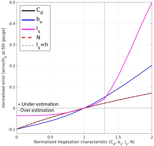
FIGURE 4. Sensitivity of the model to vegetation characteristics (C_d, b_v, l_s, and N, normalized by the observed values) for Case 1 (see Table 1) in terms of mean error normalized by the significant wave height value at the 5th gauge.

3.2 Field Case (September 17–30, 2017)

A field case study was performed using data collected in Magothy Bay, located in Northampton County, Virginia, United States. The Magothy Bay Natural Area Preserve encompasses woodlands, forested wetlands, and extensive salt marshes. The location of the study area (A) is shown in Figure 5. Eight low-frequency water level gauges and eight high-frequency (4 Hz) wave gauges were deployed along two transects, as shown in box B. The transects are perpendicular to the coastline. The first gauges on each transect are deployed bayward of the marsh; therefore, they remain submerged and measure the entire tidal cycles. On each transect, three more water levels and three wave gauges were on the marsh surface, so they become wet during high tides or in stormy conditions. The vegetation characteristics, including stem height, density, and diameter, were measured across the marsh in a field campaign led by George Mason University. Figure 6 shows vegetation sampling, including height, density, and diameter. Additional details on the field data collection can be found in Garzon et al. (2019). We have selected hurricanes Jose and Maria (2017) to verify the wave–vegetation sink term implementation in the WW3 model due to the availability of observations and atmospheric forcing and proximity of hurricane tracks to the study area.

FIGURE 5

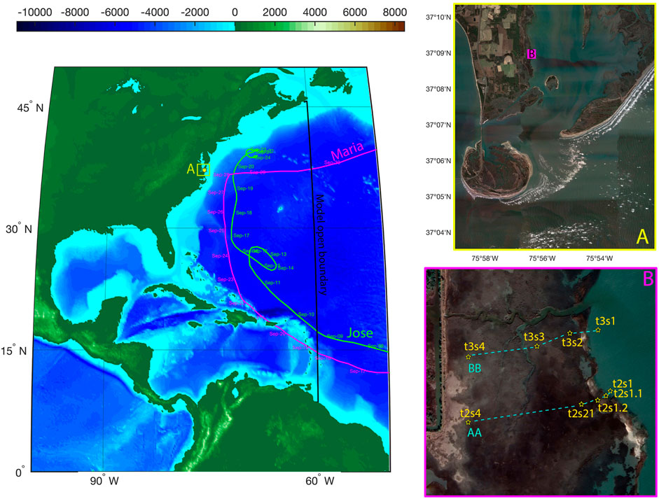
FIGURE 5. Numerical domain extent for the east coast of the United States. The black line shows the open boundaries. The best tracks with time tags of hurricanes Maria and Jose (2017) are shown by magenta and green lines, respectively. The zoom-in windows in Magothy Bay and the locations of wave and water level gauges are shown in the left-hand side panels.

FIGURE 6

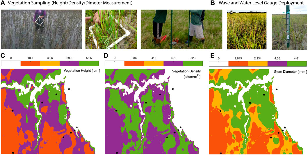
FIGURE 6. Field measurements for vegetation sampling (A) and wave and water level gauges deployment/survey (B). Spatial distribution of vegetation height (C), vegetation density (D), and stem diameters (E) in Magothy Bay.

3.2.1 Hurricane Jose (5–22 September 2017)

On 5 September, a week after the genesis of a tropical wave near the west coast of Africa, Jose developed into a tropical storm. Jose was a classic, long-lived Cape Verde hurricane that reached Category 4 strength (on the Saffir–Simpson Hurricane Wind Scale) east of the Leeward Islands on 8 September, but fortunately, it spared the Irma-ravaged islands of the northeastern Caribbean Sea. Jose made a clockwise loop over the southwestern Atlantic and then meandered off the coast of New England as a tropical storm for several days. Jose produced tropical-storm-force winds and minor coastal flooding along portions of the mid-Atlantic and southern New England coastline. Jose was directly responsible for one death, with damage of $2.84 million (2017 USD). It was the 10th named storm, fifth hurricane, and third major hurricane of the 2017 Atlantic hurricane season.

3.2.2 Hurricane Maria (16–30 September 2017)

On 12 September, a Cape Verde tropical wave later named Hurricane Maria was generated on the west coast of Africa, swept westward over the Atlantic, and formed a tropical depression about 580 nautical miles east of Barbados on 16 September (49.7°W, 12.2°N), reaching Category 5 intensity (Saffir–Simpson Hurricane Wind Scale) just before making landfall on Dominica on 18 September and high-end Category 4 hurricane by the time it struck Puerto Rico on 20 September. Maria gradually weakened over the Bahamas, swept eastward over the open Atlantic, and dissipated by 2 October. Maria was directly responsible for 3,059 deaths and indirectly responsible for further 82 fatalities, with damage of $91.61 billion (2017 USD), mostly in Puerto Rico. Maria was the most intense tropical cyclone worldwide in 2017, the 13th named storm, 8th consecutive hurricane, 4th major hurricane, 2nd Category 5 hurricane, and deadliest storm of the extremely active 2017 Atlantic hurricane season. The best tracks of the Jose and Maria path are given in Figure 5.

We have used the Hurricane Weather Research and Forecasting (HWRF) model (Ma et al., 2020) to provide winds and atmospheric pressures to force ADCIRC (Luettich et al., 1992) and WW3 models. HWRF has movable multilevel nesting technology and is designed for extreme events such as hurricanes. The model runs on a stationary parent and two movable nest domains. The parent domain covers 77.2° × 77.2° with 13.5 km resolution on a rotated latitude/longitude E-staggered grid. The middle nest domain, of about 17.8° × 17.8° with 4.5 km resolution, and the inner nest domain, of about 5.9° × 5.9° with 1.5 km resolution, move along with the storm using two-way interactive nesting. The hourly data are extracted for wind speed at 10 m elevation and pressure at MSL (see Abdolali et al. (2020) and Abdolali et al. (2021) for more information on the HWRF model and forcing data preparation).

The extent of an unstructured grid is shown in Figure 5. This grid is generated in accordance with enhancement in grid resolution and size in the study area down to 20 ∼ m coastal resolution. Such a resolution is required to represent complex marsh geometry (Deb et al., 2022b). We first conducted simulations with the ADCIRC model to prepare water level and current fields for WW3. Then, two sets of WW3 simulations were performed, forced by a wind from HWRF, water level, and current from the ADCIRC model. In the first simulation, the wave–vegetation sink term was deactivated (VEG0). In the second simulation, the VEG1 sink term was activated. For this simulation, spatially variable vegetation characteristics were used in the model.

In the wave model simulations, the model resolves the source spectrum with frequencies between 0.05 and 0.9597 Hz, divided into 32 spectral bands with an increment factor of 1.1 and 36 directions with a 10° increment. The boundary conditions are imposed at the eastern open boundary nodes of the unstructured mesh to include the effect of a distantly generated swell extracted from a global simulation on a structured grid with 0.5°, forced by the GFS wind field. In addition (Ardhuin et al., 2010), source term parameterizations (ST4), nonlinear wave-wave interaction using the discrete interaction approximation, DIA (Hasselmann et al., 1985), moving bottom friction (SHOWEX-BT4) (Ardhuin et al., 2003), depth-limited breaking based on Battjes–Janssen formulation (DB1) (Battjes and Janssen, 1978), nonlinear triad interactions (Lumped Triad Interaction method LTA) (Eldeberky and Battjes, 1996), and reflection by the coast (REF1) (Ardhuin and Roland, 2012) have been used for computations. The domain decomposition parallelization and the implicit numerical scheme are utilized for these simulations to avoid small time step in the explicit scheme, mandated by small grid resolution in the Magothy bay area (∼20 m) (Abdolali et al., 2020).

We compared the time series of storm surge and wave model outputs at pressure gauge locations (Figure 5D). The results are shown in Figure 7 for transect AA and Figure 8 for transect BB as time series of water level (η) from the storm surge model and significant wave height (H_s) from WW3. The gauges are sorted by proximity to the bay from top to bottom for each transect. In each panel, the observed and modeled water levels are shown by black and red lines, respectively. Wave observations and model outputs without vegetation sink term (VEG0) and with vegetation sink term (VEG1) are shown by blue, magenta, and green lines, respectively. Overall performance at pressure gauge locations is shown in the Taylor diagrams presented in Figure 9, combining standard deviation (σ), the root mean square deviation (RMSD), and correlation coefficient (CC) for the observation and model outputs. For water level η, the normalized standard deviation (σ) varies between 1.05 and 1.51, whereas the RMSD range is 0.42–0.87. The correlation coefficient (CC) range is 0.83–0.92. A similar correlation coefficient is observed for the significant wave height time series at wave gauge locations within the ranges of 0.51–0.88 and 0.52–0.89 for VEG0 and VEG1 sink terms, respectively. However, a substantial improvement is achieved with the activation of the vegetation sink term for the standard deviation from the range of 1.19–20.81 to 1.09–2.54. Similarly, the RMSD improved from 0.55–20.18 to 0.54–2.18.

FIGURE 7

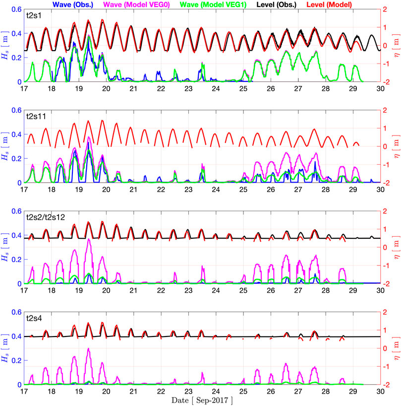
FIGURE 7. Wave and storm surge Models’ validation at the wave and water level gauges locations (transect AA) for significant wave height H_s(observation: blue; WW3 without wave–vegetation interaction: magenta; and WW3 with wave–vegetation interaction: green) and water level elevation η (observation: black; and ADCIRC: red).

FIGURE 8

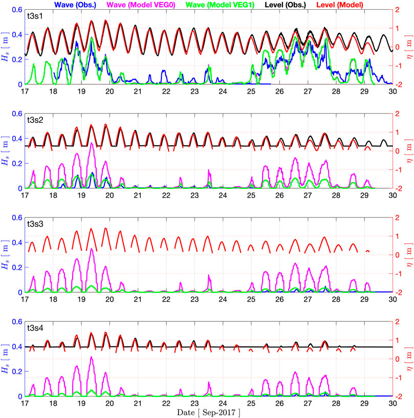
FIGURE 8. Wave and storm surge Models’ validation at the wave and water level gauges locations (transect BB) for significant wave height H_s(observation: blue; WW3 without wave–vegetation interaction: magenta; and WW3 with wave–vegetation interaction: green) and water level elevation η (observation: black; and ADCIRC: red).

FIGURE 9

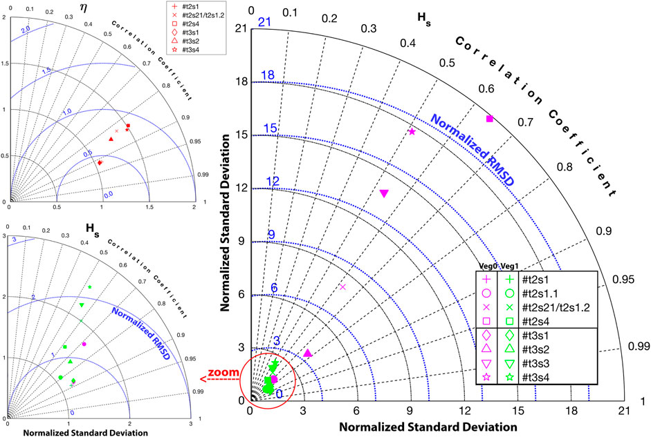
FIGURE 9. Taylor diagrams for water level (η: top left); and significant wave height (H_s: right and bottom left (zoom in) representing modeled and collected data at gauges locations (red: ADCIRC; magenta: WW3 without wave–vegetation interaction; and green: WW3 with wave–vegetation interaction) in terms of the Pearson correlation coefficient, the normalized root mean square deviation (RMSD), and the normalized standard deviation σ.

From the linear regression analysis, a slight underestimation of water level by ADCIRC is observed with a skill of 0.97, whereas WW3 overestimates the significant wave height with skills of 1.17 without the vegetation sink term and 1.04 with the vegetation sink term (Figure 10).

FIGURE 10

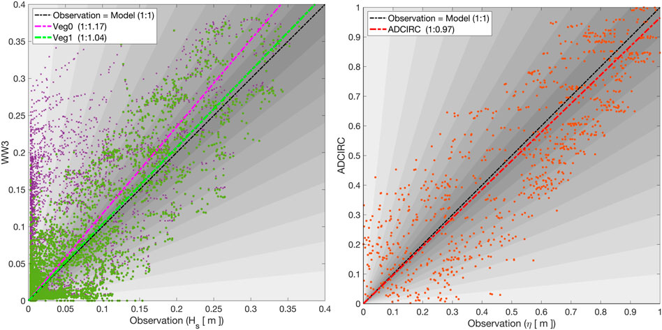
FIGURE 10. Linear regression comparison between collected data versus WW3 (significant wave height H_s: left) and ADCIRC (water elevation η: right) models. The linear regression (dotted-dashed lines) is shown in each subplot.

Wave height significantly improved due to wave–vegetation interaction. Figure 11 represents the maximum wave height during the whole simulation (17–30 September) between VEG0 and VEG1 cases.

FIGURE 11

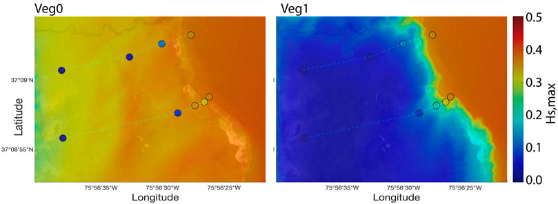
FIGURE 11. Wave model sensitivity to wave–vegetation interaction in terms of the spatial distribution of the envelope of significant wave height H_s, extracted from the model without wave–vegetation interaction (left) with wave–vegetation interaction (right). The observed maximum values at wave gauge locations are shown with the circles.

4 Summary and Conclusion

This study implemented wave–vegetation interaction in the WW3 model. The application is examined using a standard laboratory flume case for wave dissipation due to homogeneous vegetation fields. Different submergence ratios, densities were examined for single and double-peaks incident waves. The drag coefficients C_d were calculated using the empirical relationship based on Keulegan–Carpenter KC and Reynolds Re numbers, considering the correction due to the canopy submergence.

In addition to controlled laboratory experiments, we validated the model for a field application with spatially variable vegetation fields in a vegetated marshland during Hurricanes Jose and Maria, 2017. A well-known atmospheric model designed for hurricane modeling (HWRF) is used to drive the storm surge model (ADCIRC) to provide water level and current fields and the spectral wave model (WW3). These wind, current, and water level inputs were used to drive WW3 on a high-resolution triangular mesh with a ∼1 km resolution near the coast of the East Coast of the United States and a nominal resolution of $\sim 20m$ in the Magothy Bay where wave height observations were available for validation. Such a resolution is required for resolving wave action in complex marsh environments (Deb et al., 2022a). WW3 simulations were conducted with the domain decomposition parallelization algorithm and the implicit numerical solver (Abdolali et al., 2020), making it possible to run the model on a high-resolution grid efficiently. The model skills and improvement due to the vegetation sink terms were examined and discussed using time series of high-frequency pressure gauges. We conclude that the wave attenuation due to vegetation is significant in marsh environments, and neglecting the vegetation sink term leads to a significant bias in the model outputs and observations. It is shown that WW3 skills are improved over areas with vegetation, with sufficient grid resolution and proper representation of spatially variable vegetation fields. Designing and evaluating wetlands as nature-based flood risk reduction features require accurate modeling of wave dissipation by vegetation. Updated WW3 with the vegetation sink term coupled with a storm surge provides the necessary capability to model wave attenuation in wetlands. Such implementation provides an opportunity to investigate the effect of seasonal variability of vegetation coverage on wave characteristics. Organic protection methodologies can be designed for beach and wetland erosion mitigation purposes. In addition, the changes in the stem characteristic (diameter, height, and density) and hydrodynamics can be investigated to identify the role of dry/wetland cover before, during, and after the occurrence of severe storm surges. Further improvement can be achieved by a two-way coupling between the storm surge and wave models, where depth-integrated wave radiation stresses in the presence of vegetation affect the storm surge model. In return, the updated water level and current fields derive the wave model dynamically. In this way, the model components interact with each other representing what occurs in nature (Moghimi et al., 2020).

Data Availability Statement

The datasets presented in this study can be found in online repositories. The names of the repository/repositories and accession number(s) can be found at https://github.com/NOAA-emc/ww3.

Author Contributions

AA: conceptualization, methodology, code development, data curation, visualization, validation, writing—original draft. TH: conceptualization, methodology, code development, writing—review and editing. MA: laboratory experiments, writing—original draft. AR: code development, writing—review and editing. AK: field case observation collection and simulation. JS: methodology, program management, review and editing. CF: field case observation collection, review and editing. AM: program management, methodology. MS: Software.

Conflict of Interest

AA was employed by the company I.M. Systems Group, Inc.

The remaining authors declare that the research was conducted in the absence of any commercial or financial relationships that could be construed as a potential conflict of interest.

Acknowledgments

The author wishes to thank Drs. Saeideh Banihashemi and Matthew Masarik for fruitful discussions. AA and AM acknowledge the support of the Consumer Option for an Alternative System to Allocate Losses (COASTAL Act) Project within National Oceanic and Atmospheric Administration (NOAA).

Publisher’s Note

All claims expressed in this article are solely those of the authors and do not necessarily represent those of their affiliated organizations or those of the publisher, the editors, and the reviewers. Any product that may be evaluated in this article, or claim that may be made by its manufacturer, is not guaranteed or endorsed by the publisher.

Supplementary Material

The Supplementary Material for this article can be found online at: https://www.frontiersin.org/articles/10.3389/fbuil.2022.891612/full#supplementary-material

References

Abdolali, A., Roland, A., van der Westhuysen, A., Meixner, J., Chawla, A., Hesser, T. J., et al. (2020). Large-scale Hurricane Modeling Using Domain Decomposition Parallelization and Implicit Scheme Implemented in Wavewatch Iii Wave Model. Coast. Eng. 157, 103656. doi:10.1016/j.coastaleng.2020.103656

CrossRef Full Text | Google Scholar

Abdolali, A., van der Westhuysen, A., Ma, Z., Mehra, A., Roland, A., and Moghimi, S. (2021). Evaluating the Accuracy and Uncertainty of Atmospheric and Wave Model Hindcasts during Severe Events Using Model Ensembles. Ocean. Dyn. 71. doi:10.1007/s10236-020-01426-9

CrossRef Full Text | Google Scholar

Anderson, M. E., and Smith, J. M. (2015). Implementation of Wave Dissipation by Vegetation in Stwave. Vicksburg, MS. ERDC/CHL CHETN-I-5.

Google Scholar

Anderson, M. E., and Smith, J. (2014). Wave Attenuation by Flexible, Idealized Salt Marsh Vegetation. Coast. Eng. 83, 82–92. doi:10.1016/j.coastaleng.2013.10.004

CrossRef Full Text | Google Scholar

Ardhuin, F., O’reilly, W., Herbers, T., and Jessen, P. (2003). Swell Transformation across the Continental Shelf. Part I: Attenuation and Directional Broadening. J. Phys. Oceanogr. 33, 1921–1939. doi:10.1175/1520-0485(2003)033<1921:statcs>2.0.co;2

CrossRef Full Text | Google Scholar

Ardhuin, F., Rogers, E., Babanin, A. V., Filipot, J.-F., Magne, R., Roland, A., et al. (2010). Semiempirical Dissipation Source Functions for Ocean Waves. Part I: Definition, Calibration, and Validation. J. Phys. Oceanogr. 40, 1917–1941. doi:10.1175/2010JPO4324.1

CrossRef Full Text | Google Scholar

Ardhuin, F., and Roland, A. (2012). Coastal Wave Reflection, Directional Spread, and Seismoacoustic Noise Sources. J. Geophys. Res. Oceans 117. doi:10.1029/2011JC007832

CrossRef Full Text | Google Scholar

Baron-Hyppolite, C., Lashley, C. H., Garzon, J., Miesse, T., Ferreira, C., and Bricker, J. D. (2019). Comparison of Implicit and Explicit Vegetation Representations in Swan Hindcasting Wave Dissipation by Coastal Wetlands in Chesapeake Bay. Geosciences 9, 1–22. doi:10.3390/geosciences9010008

CrossRef Full Text | Google Scholar

Battjes, J. A., and Janssen, J. (1978). “Energy Loss and Set-Up Due to Breaking of Random Waves,” in Coastal Engineering 1978, 569–587. doi:10.1061/9780872621909.034

CrossRef Full Text | Google Scholar

Bender, C., Smith, J. M., Kennedy, A., and Jensen, R. (2013). Stwave Simulation of Hurricane Ike: Model Results and Comparison to Data. Coast. Eng. 73, 58–70. doi:10.1016/j.coastaleng.2012.10.003

CrossRef Full Text | Google Scholar

Bryant, M. A., and Jensen, R. E. (2017). Application of the Nearshore Wave Model Stwave to the North Atlantic Coast Comprehensive Study. J. Waterw. Port, Coast. Ocean Eng. 143, 04017026. doi:10.1061/(asce)ww.1943-5460.0000412

CrossRef Full Text | Google Scholar

Chatagnier, J. (2012). The Biomechanics of Salt Marsh Vegetation Applied to Wave and Surge Modeling. Baton Rouge, LA: Louisiana State University. Ph.D. thesis.

Google Scholar

Chow, V. T. (1959). Open-channel Hydraulics. McGraw-Hill Book Company, Inc.

Google Scholar

Dalrymple, R. A., Kirby, J. T., and Hwang, P. A. (1984). Wave Diffraction Due to Areas of Energy Dissipation. J. Waterw. Port, Coast. Ocean Eng. 110, 67–79. doi:10.1061/(asce)0733-950x(1984)110:1(67)

CrossRef Full Text | Google Scholar

Deb, M., Abdolali, A., Kirby, J. T., Shi, F., Guiteras, S., and McDowell, C. (2022b). Sensitivity of Tidal Hydrodynamics to Varying Bathymetric Configurations in a Multi-Inlet Rapidly Eroding Salt Marsh System: A Numerical Study. Earth Surf. Process. Landforms 47, 1157–1182. doi:10.1002/esp.5308

CrossRef Full Text | Google Scholar

Deb, M., Abdolali, A., Kirby, J. T., and Shi, F. (2022a). Hydrodynamic Modeling of a Complex Salt Marsh System: Importance of Channel Shoreline and Bathymetric Resolution. Coast. Eng. 173, 104094. doi:10.1016/j.coastaleng.2022.104094

CrossRef Full Text | Google Scholar

Dietrich, J. C., Westerink, J. J., Kenney, A. B., Smith, J. M., Jensen, R. E., Zijlema, M., et al. (2011). Hurricane Gustav (2008) Waves and Storm Surge: Hindcast, Synoptic Analysis, and Validation in Southern louisiana. Mon. Weather Rev. 139, 2488–2522. doi:10.1175/2011MWR3611.1

CrossRef Full Text | Google Scholar

Eldeberky, Y., and Battjes, J. A. (1996). Spectral Modeling of Wave Breaking: Application to Boussinesq Equations. J. Geophys. Res. Oceans 101, 1253–1264. doi:10.1029/95JC03219

CrossRef Full Text | Google Scholar

Figueroa-Alfaro, R. W., van Rooijen, A., Garzon, J. L., Evans, M., and Harris, A. (2022). Modelling Wave Attenuation by Saltmarsh Using Satellite-Derived Vegetaion Properties. Ecol. Eng. 176, 106528. doi:10.1016/j.ecoleng.2021.106528

CrossRef Full Text | Google Scholar

Garzon, J. L., Miesse, T., and Ferreira, C. M. (2019). Field-based Numerical Model Investigation of Wave Propagation across Marshes in the Chesapeake Bay under Storm Conditions. Coast. Eng. 146, 32–46. doi:10.1016/j.coastaleng.2018.11.001

CrossRef Full Text | Google Scholar

Hasselmann, S., Hasselmann, K., Allender, J., and Barnett, T. (1985). Computations and Parameterizations of the Nonlinear Energy Transfer in a Gravity-Wave Specturm. Part II: Parameterizations of the Nonlinear Energy Transfer for Application in Wave Models. J. Phys. Oceanogr. 15, 1378–1391. doi:10.1175/1520-0485(1985)015<1378:CAPOTN>2.0.CO;2

CrossRef Full Text | Google Scholar

Hope, M. E., Westerink, J. J., Kennedy, A. B., Kerr, P. C., Dietrich, J. C., Dawson, C., et al. (2013). Hindcast and Validation of Hurricane Ike (2008) Waves, Forerunner, and Storm Surge. J. Geophys. Res. Oceans 118, 4424–4460. doi:10.1002/jgrc.20314

CrossRef Full Text | Google Scholar

Jacobsen, N. G., Bakker, W., Uijttewaal, W. S. J., and Uittenbogaard, R. (2019). Experimental Investigation of the Wave-Induced Motion of and Force Distribution along a Flexible Stem. J. Fluid Mech. 880, 1036–1069. doi:10.1017/jfm.2019.739

CrossRef Full Text | Google Scholar

Kobayashi, N., Raichle, A. W., and Asano, T. (1993). Wave Attenuation by Vegetation. J. Waterw. port, Coast. ocean Eng. 119, 30–48. doi:10.1061/(asce)0733-950x(1993)119:1(30)

CrossRef Full Text | Google Scholar

Lawler, S., Haddad, J., and Ferreira, C. M. (2016). Sensitivity Considerations and the Impact of Spatial Scaling for Storm Surge Modeling in Wetlands of the Mid-atlantic Region. Ocean Coast. Manag. 134, 226–238. doi:10.1016/j.ocecoaman.2016.10.008

CrossRef Full Text | Google Scholar

Losada, I. J., Maza, M., and Lara, J. L. (2016). A New Formulation for Vegetation-Induced Damping under Combined Waves and Currents. Coast. Eng. 107, 1–13. doi:10.1016/j.coastaleng.2015.09.011

CrossRef Full Text | Google Scholar

Luettich, R. A., Westerink, J. J., Scheffner, N. W., et al. (1992). Adcirc: An Advanced Three-Dimensional Circulation Model for Shelves, Coasts, and Estuaries. Report 1, Theory and Methodology of Adcirc-2dd1 and Adcirc-3dl. Vicksburg, MS.

Google Scholar

Luhar, M., Infantes, E., and Nepf, H. (2017). Seagrass Blade Motion under Waes and its Impact on Wave Decay. J. Geophys. Res. Oceans 122, 3736–3752. doi:10.1002/2017jc012731

CrossRef Full Text | Google Scholar

Ma, Z., Liu, B., Mehra, A., Abdolali, A., van der Westhuysen, A., Moghimi, S., et al. (2020). Investigating the Impact of High-Resolution Land–Sea Masks on Hurricane Forecasts in Hwrf. Atmosphere 11. doi:10.3390/atmos11090888

CrossRef Full Text | Google Scholar

Mendez, F. J., and Losada, I. J. (2004). An Empirical Model to Estimate the Propagation of Random Breaking and Nonbreaking Waves over Vegetation Fields. Coast. Eng. 51, 103–118. doi:10.1016/j.coastaleng.2003.11.003

CrossRef Full Text | Google Scholar

Mendez, F. J., Losada, I. J., and Losada, M. A. (1999). Hydrodynamics Induced by Wind Waves in a Vegetation Field. J. Geophys. Res. Oceans 104, 18383–18396. doi:10.1029/1999jc900119

CrossRef Full Text | Google Scholar

Moghimi, S., Van der Westhuysen, A., Abdolali, A., Myers, E., Vinogradov, S., Ma, Z., et al. (2020). Development of an Esmf Based Flexible Coupling Application of Adcirc and Wavewatch Iii for High Fidelity Coastal Inundation Studies. J. Mar. Sci. Eng. 8. doi:10.3390/jmse8050308

CrossRef Full Text | Google Scholar

Ozeren, Y., Wren, D. G., and Wu, W. (2014). Experimental Investigation of Wave Attenuation through Model and Live Vegetation. J. Waterw. Port, Coast. Ocean Eng. 140, 04014019. doi:10.1061/(asce)ww.1943-5460.0000251

CrossRef Full Text | Google Scholar

Phan, K. L., Stive, M. J. F., Zijlema, M., Truong, H. S., and Aarninkhof, S. G. J. (2019). The Effects of Wave Non-linearity on Wave Attenuation by Vegetation. Coast. Eng. 147, 63–74. doi:10.1016/j.coastaleng.2019.01.004

CrossRef Full Text | Google Scholar

Roland, A. (2008). Development of WWM II: Spectral Wave Modelling on Unstructured Meshes. Darmstadt, Germany: Technische Universität Darmstadt, Institute of Hydraulic and. Ph.D. thesis, Ph. D. thesis.

Google Scholar

Smith, J. M., Bryant, M. A., and Wamsley, T. V. (2016). Wetland Buffers: Numerical Modeling of Wave Dissipation by Vegetation. Earth Surfaces Process. Landforms 41, 847–854. doi:10.1002/esp.3904

CrossRef Full Text | Google Scholar

Suzuki, T., Zijlema, M., Burger, B., Meijer, M. C., and Narayan, S. (2012). Wave Dissipation by Vegetation with Layer Schematization in Swan. Coast. Eng. 59, 64–71. doi:10.1016/j.coastaleng.2011.07.006

CrossRef Full Text | Google Scholar

Tang, J., Shaodong, S., and Wang, H. (2015). Numerical Model for Coastal Wave Propagation through Mild Slope Zone in the Presence of Rigid Vegetation. Coast. Eng. 97, 53–59. doi:10.1016/j.coastaleng.2014.12.006

CrossRef Full Text | Google Scholar

Tempest, J. A., Moller, I., and Spencer, T. (2015). A Review of Plant-Flow Interactions on Salt Marshes: The Importance of Vegetation Structure and Plant Mechanical Characteristics. WIREs Water 2, 669–681. doi:10.1002/wat2.1103

CrossRef Full Text | Google Scholar

Van Rooijen, A. A., Van Thie de Vries, J. S. M., McCall, R. T., Van Dongeren, A. R., Roelvink, J. A., and Reniers, A. J. H. M. (2015). “Modeling of Wave Attenuation by Vegetation with Xbeach,” in E-proceedings of the 36th IAHR World Congress. Hague, Netherlands.

Google Scholar

van Veelen, T. J., Fairchild, T. P., Reeve, D. E., and Karunarathna, H. (2020). Experimental Study on Vegetation Flexibility as Control Parameter for Wave Damping and Velocity Structure. Coast. Eng. 157, 103648. doi:10.1016/j.coastaleng.2020.103648

CrossRef Full Text | Google Scholar