 Daisuke Murakami
 Takahiro Yoshida
 Yoshiki Yamagata3
94% of researchers rate our articles as excellent or good
Learn more about the work of our research integrity team to safeguard the quality of each article we publish.
Find out more
ORIGINAL RESEARCH article
Front. Built Environ., 22 October 2021
Sec. Urban Science
Volume 7 - 2021 | https://doi.org/10.3389/fbuil.2021.760306
This article is part of the Research TopicTheories, Models and Observations of Urban Spatial Expansion: Patterns, Drivers, Impacts and Vulnerabilities of Future Urban WorldsView all 5 articles
Historical and future spatially explicit population and gross domestic product (GDP) data are essential for the analysis of future climate risks. Unlike population projections that are generally available, GDP projections—particularly for scenarios compatible with shared socioeconomic pathways (SSPs)—are limited. Our objective is to perform a high-resolution and long-term GDP estimation under SSPs utilizing a wide variety of geographic auxiliary information. We estimated the GDP in a 1/12-degree grid scale. The estimation is done through downscaling of historical GDP data for 1850–2010 and SSP future scenario data for 2010–2100. In the downscaling, we first modeled the spatial and economic interactions among cities and projected different future urban growth patterns according to the SSPs. Subsequently, the projected patterns and other auxiliary geographic data were used to estimate the gridded GDP distributions. Finally, the GDP projections were visualized via three-dimensional mapping to enhance the clarity for multiple stakeholders. Our results suggest that the spatial pattern of urban and peri-urban GDP depends considerably on the SSPs; the GDP of the existing major cities grew rapidly under SSP1, moderately grew under SSP 2 and SSP4, slowly grew under SSP3, and dispersed growth under SSP5.
Building urban resilience against climate risks including flooding, storm, and heatwave, is an emergent task across the world. Future scenarios for population, economic productivity, and other socio-economic variables are required to estimate climate-related damage in the future and to consider countermeasures. IPCC (Inter-governmental Panel on Climate Change) published Shared Socioeconomic Pathways (SSP), which are future scenarios for socio-economic variables under possible future developmental paths that is, sustainability (SSP1), middle of the road (SSP2), regional rivalry (SSP3), inequality (SSP4), and fossil-fueled development (SSP5) (O’Neill et al., 2014; Jones and O’Neill 2016). Roughly speaking, SSP1 assumes rapid and compact urban growth, SSP2 assumes that the current state lasts in the future, SSP3 assumes failure of globalization that leads to a lower level of economic growth and low international priority for addressing environmental concerns, SSP4 assumes increasing inequality leading to higher growth in developed countries and lower growth in less developed countries, and SSP5 assumes a fossil-fueled or car-oriented development that results in large-scale urban sprawl. Additionally, the current COVID-19 pandemic may accelerate and entrench longer-term reduction in product-trades and immigration flows. As the result, such a scenario would have parallels to the SSP3 scenario which projects slower economic growth than the other SSPs (Burgess et al., 2020).
While country-level SSPs data are available from the SSP Database (Riahi et al., 2017), climate risk considerably changes within countries. For example, flood risk of a city changes depending on whether the city is in a water-front area or not. Regional SSPs are needed to estimate climate risks in each country. With this background, country-level population scenarios have been downscaled into fine spatial grids under SSPs (Jones and O’Neill 2016; Murakami and Yamagata 2019; Wear and Prestemon 2019) and other future scenarios (Gaffin et al., 2004; Bengtsson et al., 2007; McKee et al., 2015; Yamagata et al., 2015).
By contrast, the SSP GDP scenario has rarely been downscaled, whereas GDP scenarios other than SSP have been done (Gaffin et al., 2004; Grübler et al., 2007; Fujimori et al., 2017; Kummu et al., 2018). One of the reasons for the lack of SSP GDP scenario downscaling is the difficulty compared to population downscaling. In the case of population downscaling, high-resolution population estimates from past to present are available; fine-grained population projection is readily obtained by extrapolating the past trend. Unfortunately, such extrapolation is not possible for GDP because of the lack of such past-to-present data. To the best of our knowledge, Murakami and Yamagata (2019) is the only one downscaling SSP GDP scenarios into fine grids. They estimated the explanatory power of each auxiliary geographic data (e.g., urban population, road network, distance to the ocean) on GDP distribution using an ensemble learning technique, and country GDPs were downscaled into grids based on the results. Unfortunately, their database has the following limitations. First, their assumed spatial resolution of 0.5-degree grids is not fine enough to estimate the climate risk of individual cities. 0.5-degree nearly equals 55.83 (=111.66/2) km around the equator while 42.64 km in a 40-degree area. Multiple cities could be in one grid. Second, the authors did not consider SSP4 and SSP5. Third, their estimates are not available before 2010.
The objective of this study is to overcome these limitations. Specifically, we estimated GDPs by 1/12 grids for the period between 1850 and 2100 by 10 years by downscaling actual GDPs between 1850 and 2010 and projected GDPs under SSPs 1–5 between 2020 and 2100.
We downscaled country GDPs into 1/12-degree grids. The downscaling was performed from 1850 to 2100 by 10 years. The procedure for each year after 2020 is summarized in Figure 1. Table 1 summarizes the input data. In order to project the extent of urbanization in the future, we first estimated the growth of individual cities under each SSP ((1) of Figure 1). Then, based on the results, we projected the urbanization potential by the grids under each SSP ((2) of Figure 1). Note that we cannot consider COVID-19 because the SSPs, which we will downscaled, ignore it. Consideration of COVID-19 will be an important next topic.
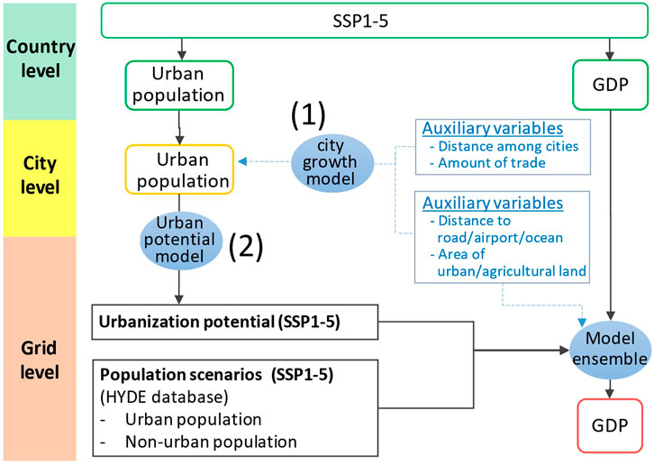
FIGURE 1. Procedure for population and GDP downscaling (after 2020). Variables by countries, cities, and grids are coloured by green, yellow, and red, respectively. As this figure shows, the urban population was downscaled from countries to cities to estimate the potential of urbanization by the grids. The estimated potential under SSP 1–5 was used together with the grid population estimates, and other auxiliary variables in the model ensemble-based downscaling.
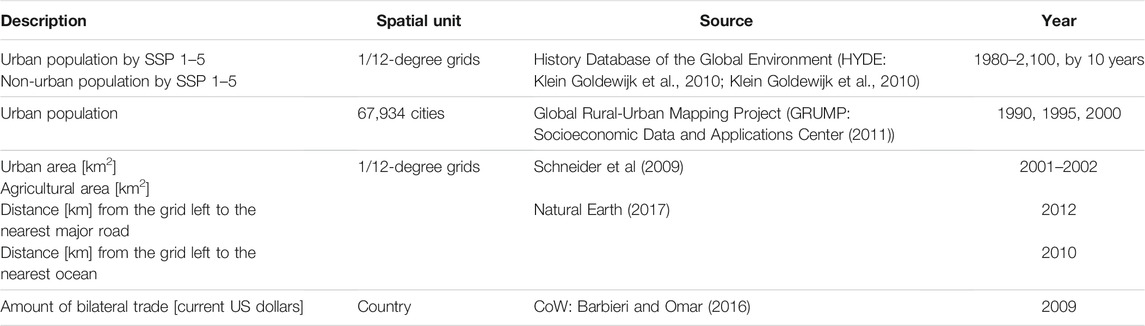
TABLE 1. Auxiliary variables.
The following model was used for (1) the urban growth projection ((1) in Figure 1):
where
In summary, Eq. 1 estimates the 5-year population growth of individual cities based on international and domestic socio-economic interaction, geographic proximity, the population of the previous 5 years
The coefficients
Based on SSP storylines, we assumed different values for the city-wise interaction parameters
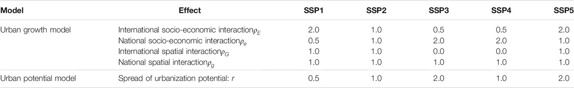
TABLE 2. Assumptions for the parameters in 2,100 in the urban growth model (SSP2: 1.0).
The projected city-wise populations were used to estimate the urbanization potential by the grid ((2) in Figure 1). The potential
The gridded urbanization potential under SSPs, which was estimated in Projection of urbanization projection, was used as an auxiliary variable for the GDP downscaling ((2) in Figure 1). The other auxiliary variables are as follows: urban and non-urban populations by the 1/12 grids by SSPs, urban area, agricultural area, accessibility measures including distance to the nearest major road, airport, and ocean. See Table 1 for further detail.
Generally, downscaling is performed by proportionally distributing the target variable according to an auxiliary weight variable such as population and area. For accurate downscaling, it is crucially important to appropriately specify the weight variable. We optimize the weight variable using a gradient boosting technique. The weight in the g-th grid is defined by
Figures 2, 3 plot the gridded GDP estimates in 2010 and 2100 under SSP 1-5 in Europe and Eastern Asia, respectively. Our estimates produced considerably different map patterns across SSPs. SSPs 1 and 2 indicated a higher level of urban growth within the existing major cities. Still, growth in non-urban areas were as slow as SSP 3, which is a less urbanized scenario. This tendency was prominent in SSP1. These results are consistent with the assumption of rapid and compact urban growth in the SSP 1 scenario. Conversely, SSP 5 resulted in severe urban expansion. Because SSP 5 assumes a fossil-fueled development that yields widespread road networks, this result is reasonable. SSPs 3 and 4 had a lower level of urban growth, especially in Asian countries because of the assumption of the limited globalization. SSP 3 results in a notably small GDP growth nearby major cities (e.g., London, Paris, Shanghai). All these results are consistent with the assumptions underlying SSPs.
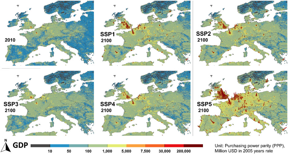
FIGURE 2. Downscaled gross productivities in 2010 and those in 2,100 the SSP 1–5 (Europe).
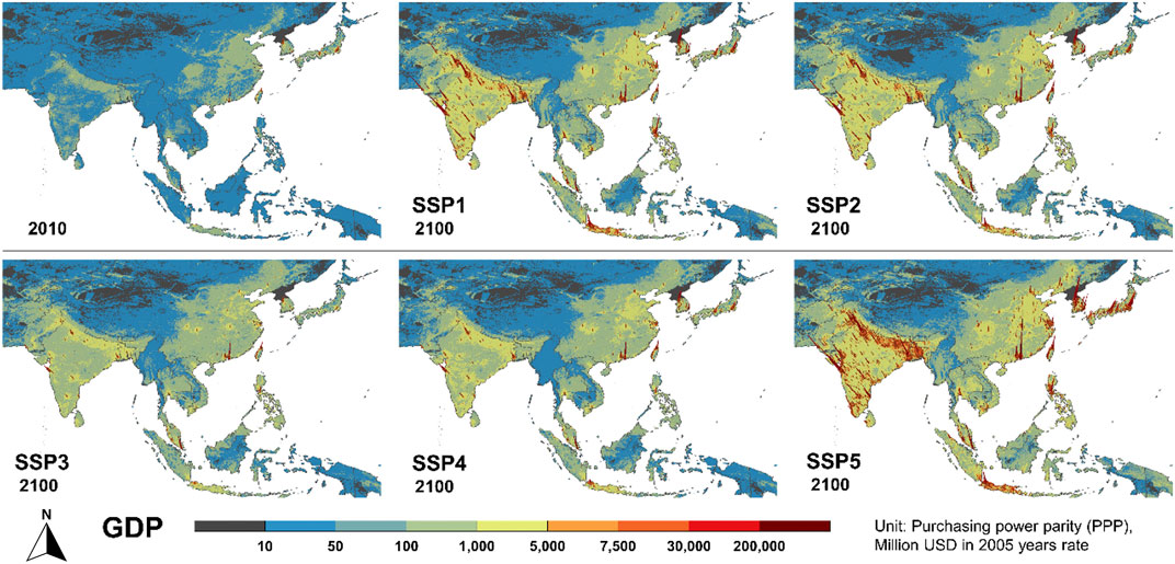
FIGURE 3. Downscaled gross productivities in 2010 and 2,100 in SSP 1–5 (Eastern Asia).
This section examines the accuracy of the downscaling. We first compared our GDP estimates with those of Kummu et al (2018), which were calculated based on a time-series modelling of sub-national GDPs and downscaling based on gridded population estimates. Here, GDP estimates in 2010 by 1/12-degree grids, which are available in both our estimates and Kummu et al (2018)’s estimates are compared. The study areas for the comparison include the NUTS 2 regions, which usually have populations between 800,000 and 3 million people, in Europe (Eurostat 2020), United States excluding Hawaii and Alaska (United States Cencus Bureau 2020), and Japan (Statistics Bureau of Japan 2015).
Figure 4 compares our GDP estimates with the gridded GDP of Kummu et al (2018) in 2010. This plot suggests that these estimates have similar patterns. The R-squares between the two GDP estimates are 0.720 (Europe), 0.885 (United States), and 0.834 (Japan), respectively, confirming the similarity of these estimates. On the other hand, our estimates have lower GDP values than Kummu et al (2018) in developed areas. This is because we distribute national GDP for not only developed areas but also the neighbouring areas based on the distribution weight depending on auxiliary attributes (urbanization potentials, road networks…), which is optimized by the gradient boosting technique. In other words, the lower GDP value in developed area is attributable to our optimized distribution weights allocating more GDP on the neighboring areas.
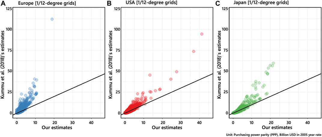
FIGURE 4. Comparison of our GDP estimates with Kummu et al (2018).
Then, to examine consistency of our estimates with actual GDP, we compared our estimates for 2010 with the regional GDPs in the NUTS 2 regions, the 49 states of the United States, and the prefectural GDP in Japan. In each region, our estimates were aggregated into the aggregate units which these databases assume. Figure 5 summarizes the comparison results. The R-squares were 0.685 in the NUTS2 regions, 0.937 in the United States, and 0.735 in the prefectures in Japan. The results suggest that our estimates are fairly accurate despite the fact that our downscaling did not use any regional GDP statistics.
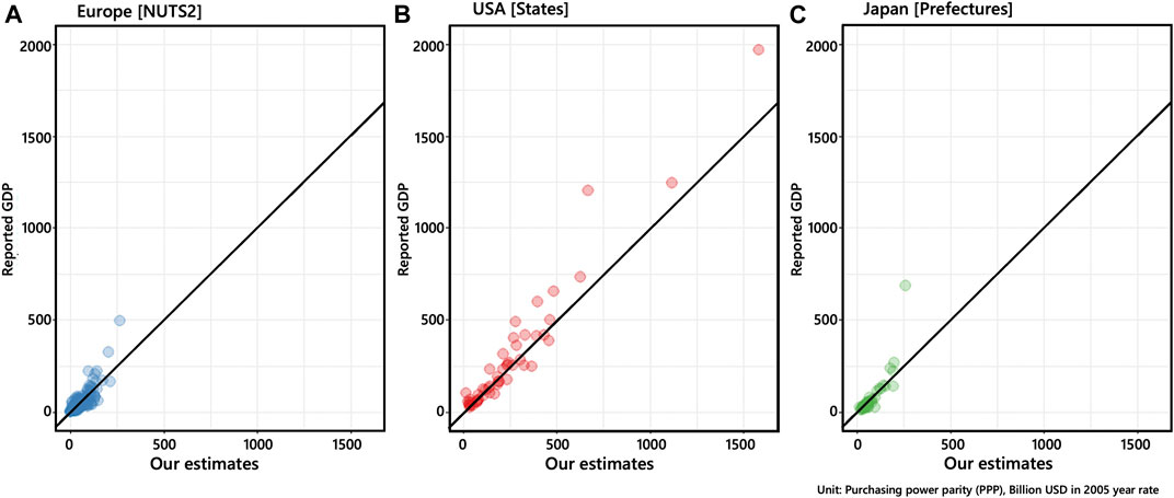
FIGURE 5. Comparison of our GDP estimates with the reported GDP in 2010. For comparison, our estimates were aggregated.
The downscaled GDP data is potentially useful for decision making toward sustainable development. For example, by spatially overlaying hazard map with our estimates, possible economic loss due to flood, earthquake, and other natural disasters can be estimated. The result will be useful for disaster risk management. The estimated GDPs are also useful to estimate the map pattern of carbon emissions in the future and consider policies toward low carbon development.
SSP scenarios on population and GDP used by IPCC are central for the analysis of future climate risks and policy. Population projections are generally available; however, GDP projections—particularly for scenarios compatible with SSPs—are limited. In this study, we estimated the GDP in a 1/12-degree grid scale for the period of 1850–2100 in 10-year intervals by using spatial econometric based downscaling algorithm. Our results suggest that the spatial pattern of urban and peri-urban GDP depends considerably on the SSPs; e.g., the urban GDP under SSP1 grew rapidly within the existing major cities. These cities grew moderately under SSP2 and SSP4. In contrast, that under SSP3 exhibited a lower growth level, and that under SSP5 exhibited extreme dispersion.
The major improvements relative to Murakami and Yamagata (2019) are as follows: (i) GDPs by the 1/12 grids, which are considerably finer than their assumed grids, were estimated; (ii) GDPs were downscaled under SSP4 and SSP5; GDPs were downscaled not only in the future but also in the past. The high resolution and long-term GDP estimates will be useful to analyse the relationship between urban development and climate change in detail.
Some important issues remain in this study. First, spatially finer auxiliary data are needed to sophisticate our downscaling approach. For example, microscale urban data, such as industrial structure, detailed road network, and traffic volume, are required to consider urban phenomena including industrial agglomeration, growth of transportation networks. Consideration of the birth of new cities is also an important topic. Since consideration of these factors can increase the uncertainty of downscaling, it is crucial to employ a robust estimation approach like Bayesian estimation (see, e.g., Raftery et al., 2012 for population projection).
Second, assumptions for the parameters in the urban growth model should be enhanced. As discussed in Hausfather and Peters (2020), and Pielke and Ritchie (2020), high emission scenarios should not be used as the reference baseline in climate research. Future scenario should be developed considering a wider range of assumptions due to the uncertainty in urban growth. Another important topic is to estimate the difference in urban metabolism pattern in each country/city. For instance, road density might have stronger impact on GDP in United States, which has developed heavily dependent on cars, while weaker impact in Europe. Unfortunately, our model, which assumes the relative importance of each auxiliary variable as constant across countries, ignores such spatial heterogeneity. Estimation of the heterogeneity for example by incorporating our model with country-level local models is an important next subject.
It is also important to consider the impact of COVID-19 pandemic that may change economic systems (Burgess et al., 2020). Spatially fine scale projection can be useful for policymaking for city-level economic development and climate risk mitigation. It is important to update scenario assumptions considering uncertainty relating COVID-19 and other factors.
The datasets presented in this study can be found in online repositories. The names of the repository/repositories and accession number(s) can be found below: https://doi.org/10.6084/m9. figshare.12016506. The usage note of the data and the visualization is also available online. Figure 6 shows a snapshot of the website. This website includes an interactive 3-dimensional visualizer. Users can zoom-in/zoom-out any region and change the colour scale. This function will help users to understand the map patterns of GDP even without downloading the data.
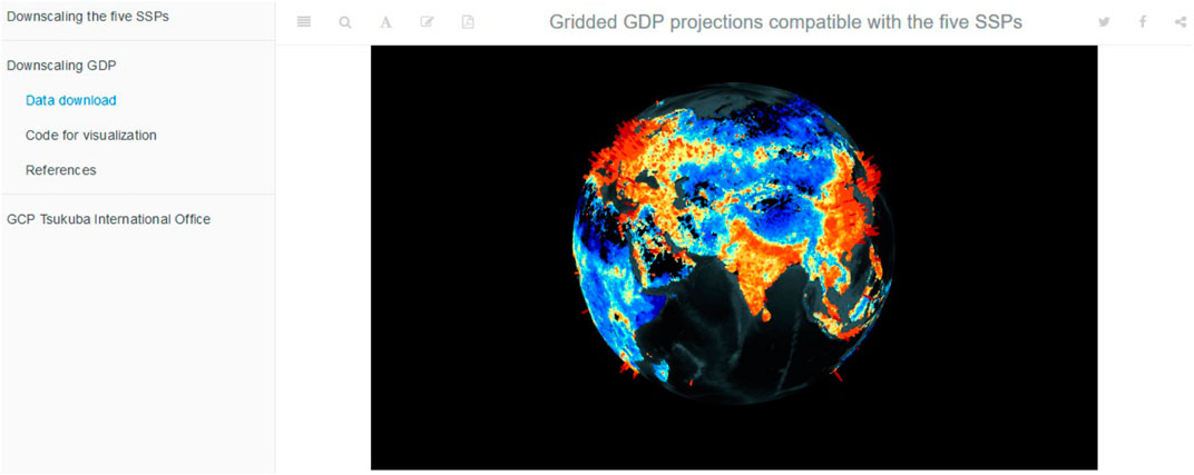
FIGURE 6. Image of the website for GDP data visualization.
DM performed the downscaling and wrote the draft. TY wrote the draft and made the website to publish the data. YY directed and managed this downscaling project.
The authors declare that the research was conducted in the absence of any commercial or financial relationships that could be construed as a potential conflict of interest.
All claims expressed in this article are solely those of the authors and do not necessarily represent those of their affiliated organizations, or those of the publisher, the editors and the reviewers. Any product that may be evaluated in this article, or claim that may be made by its manufacturer, is not guaranteed or endorsed by the publisher.
Barbieri, K., and Omar, K. (2016). Correlates of War Project Trade Data Set Codebook. Version 4.0 Available at: http://correlatesofwar.org (Accessed August 17, 2021).
Bengtsson, M., Shen, Y., and Oki, T. (2007). A SRES-Based Gridded Global Population Dataset for 1990-2100. Popul. Environ. 28, 113–131. doi:10.1007/s11111-007-0035-8
Burgess, M. G., Ritchie, J., Shapland, J., and Pielke, R. (2020). IPCC Baseline Scenarios Have Over-projected CO2 Emissions and Economic Growth. Environ. Res. Lett. 16, 014016. doi:10.1088/1748-9326/abcdd2
Eurostat (2020). Eurostat Database Online. Available at: https://ec.europa.eu/eurostat (Accessed August 17, 2021).
Fujimori, S., Abe, M., Kinoshita, T., Hasegawa, T., Kawase, H., Kushida, K., et al. (2017). Downscaling Global Emissions and its Implications Derived from Climate Model Experiments. PLoS One 12, e0169733. doi:10.1371/journal.pone.0169733
Gaffin, S. R., Rosenzweig, C., Xing, X., and Yetman, G. (2004). Downscaling and Geo-Spatial Gridding of Socio-Economic Projections from the IPCC Special Report on Emissions Scenarios (SRES). Glob. Environ. Change 14, 105–123. doi:10.1016/j.gloenvcha.2004.02.004
Grübler, A., O'Neill, B., Riahi, K., Chirkov, V., Goujon, A., Kolp, P., et al. (2007). Regional, National, and Spatially Explicit Scenarios of demograph.ic and Economic Change Based on SRES. Technol. Forecast. Soc. Change 74, 980–1029. doi:10.1016/j.techfore.2006.05.023
Hausfather, Z., and Peters, G. P. (2020). Emissions - the ‘business as Usual' story Is Misleading. Nature 577, 618–620. doi:10.1038/d41586-020-00177-3
Jones, B., and O’Neill, B. C. (2016). Spatially Explicit Global Population Scenarios Consistent with the Shared Socioeconomic Pathways. Environ. Res. Lett. 11, 084003. doi:10.1088/1748-9326/11/8/084003
Klein Goldewijk, K., Beusen, A., and Janssen, P. (2010). Long-term Dynamic Modeling of Global Population and Built-Up Area in a Spatially Explicit Way: HYDE 3.1. The Holocene 20, 565–573. doi:10.1177/0959683609356587
Klein Goldewijk, K., Beusen, A., Van Drecht, G., and De Vos, M. (2011). The HYDE 3.1 Spatially Explicit Database of Human-Induced Global Land-Use Change over the Past 12,000 Years. Glob. Ecol. Biogeogr. 20, 73–86. doi:10.1111/j.1466-8238.2010.00587.x
Kummu, M., Taka, M., and Guillaume, J. H. A. (2018). Gridded Global Datasets for Gross Domestic Product and Human Development Index over 1990-2015. Sci. Data 5, 180004. doi:10.1038/sdata.2018.4
McKee, J. J., Rose, A. N., Bright, E. A., Huynh, T., and Bhaduri, B. L. (2015). Locally Adaptive, Spatially Explicit Projection of US Population for 2030 and 2050. Proc. Natl. Acad. Sci. USA 112, 1344–1349. doi:10.1073/pnas.1405713112
Murakami, D., and Yamagata, Y. (2019). Estimation of Gridded Population and GDP Scenarios with Spatially Explicit Statistical Downscaling. Sustainability 11, 2106. doi:10.3390/su11072106
Natural Earth (2017). Available at: https://www.naturalearthdata.com/ (Accessed August 17, 2021).
O’Neill, B. C., Kriegler, E., Riahi, K., Ebi, K. L., Hallegatte, S., Carter, T. R., et al. (2014). A New Scenario Framework for Climate Change Research: the Concept of Shared Socioeconomic Pathways. Clim. Change 122, 387–400. doi:10.1007/s10584-013-0905-2
Pielke, R., and Ritchie, J. (2020). Systemic Misuse of Scenarios in Climate Research and Assessment. SSRN Electron. J., 3, 3581777. doi:10.2139/ssrn.3581777
Raftery, A. E., Li, N., Sevcikova, H., Gerland, P., and Heilig, G. K. (2012). Bayesian Probabilistic Population Projections for All Countries. Proc. Natl. Acad. Sci. 109, 13915–13921. doi:10.1073/pnas.1211452109
Riahi, K., van Vuuren, D. P., Kriegler, E., Edmonds, J., O’Neill, B. C., Fujimori, S., et al. (2017). The Shared Socioeconomic Pathways and Their Energy, Land Use, and Greenhouse Gas Emissions Implications: An Overview. Glob. Environ. Change 42, 153–168. doi:10.1016/j.gloenvcha.2016.05.009
Schneider, A., Friedl, M. A., and Potere, D. (2009). A New Map of Global Urban Extent from MODIS Satellite Data. Environ. Res. Lett. 4, 044003. doi:10.1088/1748-9326/4/4/044003
Socioeconomic Data and Applications Center (2011). Global Rural-Urban Mapping Project (GRUMPv1). Settlement Points, v1. doi:10.7927/H4M906KR (Accessed August 17, 2021).
Statistics Bureau of Japan (2015). E-Stat. Available at: https://www.stat.go.jp/english (Accessed August 17, 2021).
United States Cencus Bureau (2020). US Census. Available at: https://www.census.gov/ (Accessed August 17, 2021).
Wear, D. N., and Prestemon, J. P. (2019). Spatiotemporal Downscaling of Global Population and Income Scenarios for the United States. PLoS One 14, e0219242. doi:10.1371/journal.pone.0219242
Keywords: shared socioeconomic pathways, gross domestic product, downscale, 1/12-degree grid scale, spatial econometrics
Citation: Murakami D, Yoshida T and Yamagata Y (2021) Gridded GDP Projections Compatible With the Five SSPs (Shared Socioeconomic Pathways). Front. Built Environ. 7:760306. doi: 10.3389/fbuil.2021.760306
Received: 18 August 2021; Accepted: 05 October 2021;
Published: 22 October 2021.
Edited by:
Peter John Marcotullio, Hunter College (CUNY), United StatesReviewed by:
Mahua Mukherjee, Indian Institute of Technology Roorkee, IndiaCopyright © 2021 Murakami, Yoshida and Yamagata. This is an open-access article distributed under the terms of the Creative Commons Attribution License (CC BY). The use, distribution or reproduction in other forums is permitted, provided the original author(s) and the copyright owner(s) are credited and that the original publication in this journal is cited, in accordance with accepted academic practice. No use, distribution or reproduction is permitted which does not comply with these terms.
*Correspondence: Daisuke Murakami, ZG11cmFrYUBpc20uYWMuanA=
Disclaimer: All claims expressed in this article are solely those of the authors and do not necessarily represent those of their affiliated organizations, or those of the publisher, the editors and the reviewers. Any product that may be evaluated in this article or claim that may be made by its manufacturer is not guaranteed or endorsed by the publisher.
Research integrity at Frontiers
Learn more about the work of our research integrity team to safeguard the quality of each article we publish.