A Performance-Based Wind Engineering Framework for Engineered Building Systems Subject to Hurricanes

Over the past decade, significant research efforts have been dedicated to the development of performance-based wind engineering (PBWE). Notwithstanding these efforts, frameworks that integrate the damage assessment of the structural and envelope system are still lacking. In response to this need, the authors have recently proposed a PBWE framework that holistically treats envelope and structural damages through progressive multi-demand fragility models that capture the inherent coupling in the demands and damages. Similar to other PBWE methodologies, this framework is based on describing the hurricane hazard through a nominal straight and stationary wind event with constant rainfall and one-hour duration. This study aims to develop a PBWE framework based on a full description of the hurricane hazard in which the entire evolution of the storm track and time-dependent wind/rain fields is simulated. Hurricane-induced pressures impacting the building envelope are captured through the introduction of a non-stationary/-straight/-Gaussian wind pressure model. Time-dependent wind-driven rain is modeled through a computational fluid dynamics Eulerian multiphase framework with interpolation schemes for the rapid computation of wind-driven rain intensities over the building surface. Through the development of a conditional stochastic simulation algorithm, the envelope performance is efficiently characterized through probabilistic metrics associated with rare events of design interest. The framework is demonstrated through analyzing a 45-story archetype building located in Miami, FL, for which the envelope performance is estimated in terms of a suite of probabilistic damage and loss metrics. A comparative study is carried out in order to provide insights into the differences that can occur due to the use of nominal hurricane models.

1 Introduction

Performance-based design (PBD) has been widely accepted as a rational way of assessing risks to engineered facilities subjected to natural hazards (Porter, 2003). Over the past decade, significant research efforts have been placed on the development of frameworks for the performance-based assessment of wind-excited buildings (Ciampoli et al., 2011; Smith and Caracoglia, 2011; Petrini and Ciampoli, 2012; Barbato et al., 2013; Bernardini et al., 2015; Pita et al., 2016; Chuang and Spence, 2017; Cui and Caracoglia, 2018; Ierimonti et al., 2019; Micheli et al., 2019; Ouyang and Spence, 2019; Cui and Caracoglia, 2020; Ouyang and Spence, 2020; Ouyang and Spence, 2021). Most frameworks developed to date assess damage and loss to the building system based on demands estimated exclusively from the structural response (e.g., peak interstory drifts, accelerations) notwithstanding how a significant portion of envelope damage is generated from local dynamic wind pressure. In an attempt to address this, the authors have recently introduced a PBWE framework where damage is estimated through a progressive analysis in which coupled structural response and wind pressure demands are considered as input to a multi-demand fragility analysis that captures damage state interdependency (Ouyang and Spence, 2019, 2020, 2021). Similar to existing PBWE methodologies, this framework adopted a nominal hurricane hazard based on the assumption of a straight (i.e., constant wind direction) and stationary wind event of one-hour duration. The intensity of the wind event was characterized through the maximum mean hourly wind speed to occur at the building top. Likewise, the intensity of the concurrent rain event was characterized through the maximum horizontal rainfall to occur during the hurricane at the site of interest. While this nominal hurricane setting simplifies subsequent damage and loss analysis, the relative accuracy of performance assessments based on nominal hurricanes, as compared to those carried out considering the full non-straight/-stationary nature of hurricane winds and concurrent rainfall, remains unknown.

To fill this knowledge gap, this work develops a PBWE framework for the performance assessment of envelope systems based on describing the full evolution of the hurricane event through parametric hurricane models for both the wind and concurrent rainfall fields. In particular, hurricane tracks are described through the probabilistic parametric models outlined by Vickery and Twisdale (1995a); Vickery et al. (2000b); and Cui et al. (2021), while the associated wind fields are described through the two-dimensional wind field model outlined by Vickery and Twisdale (1995b); Vickery et al. (2000a); and Jakobsen and Madsen (2004). These models are subsequently combined with parametric precipitation models (e.g., Lonfat et al., 2007; Grieser and Jewson, 2012; Geoghegan et al., 2018; Snaiki and Wu, 2018; Brackins and Kalyanapu, 2020) that use as input a subset of the hurricane model parameters therefore enabling a probabilistic description of concurrent horizontal rainfall intensity. The consideration of continuously time-varying hurricane inputs (i.e., evolving storm track and horizontal rainfall intensity) requires a new set of models for the simulation of the aerodynamic loads and wind-driven rain. To this end, a novel wind-tunnel-informed non-straight/-stationary/-Gaussian wind pressure simulation framework is introduced. For the wind-driven rain, the Eulerian multiphase computational fluid dynamics (CFD) model outlined by Kubilay et al. (2013, 2015) is adopted with an interpolation scheme within the space of the wind speed and direction therefore allowing for the efficient estimation of the instantaneous rainwater deposition on the building envelope in terms of the continually varying wind speed and direction.

To demonstrate the applicability of the framework, a 45-story archetype building located in Miami, FL, is studied in terms of probabilistic performance metrics associated with envelope damages, monetary losses, and water ingress. A comprehensive comparison of the results with those obtained by considering a nominal hurricane setting is also carried out with the aim of better understanding the feasibility of using classic hurricane hazard models in the PBWE of engineered building systems.

2 The Performance-Based Wind Engineering Setting

Pioneered by the Pacific Earthquake Engineering Research (PEER) center (Porter, 2003), frameworks for probabilistic performance-based earthquake engineering have been widely adopted as the basis for developing frameworks for PBWE. The current work is developed based on the recently proposed PBWE framework outlined by Ouyang and Spence (2020), the implementation of which enables the estimation of probabilistic building envelope performance metrics of interest to stakeholders (e.g., expected repair costs, expected water ingress) based on a nominal description of the hurricane hazard. In particular, as detailed in Ouyang and Spence (2020), the framework is based on characterizing performance through solving the following probabilistic integral:

$\lambda \left(dv\right)=\int \int \int \int G\left(dv|sm\right)|dG\left(sm|R_h,{\alpha }_H,{\bar{v}}_H\right)\Vert dG\left(R_h|{\alpha }_H,{\bar{v}}_H\right)||dG\left({\alpha }_H|{\bar{v}}_H\right)\Vert d\lambda \left({\bar{v}}_H\right)|(1)$

where G(x|y) is the conditional complementary cumulative distribution function (CCDF) of random variable x given y, sm is the system measure variables (e.g., number of damaged components and amount of water ingress), R_h is the mean hourly rainfall intensity, α_H is the wind direction, ${\bar{v}}_H$ is the maximum mean hourly wind speed measured at a height of interest (e.g., building top), dv is a decision variable threshold of interest (e.g., thresholds related to repair costs, downtime, volume of water ingress), and λ is the mean annual rate of exceeding the threshold of interest, therefore resulting in $\lambda ({\bar{v}}_H)$ representing the non-directional hurricane hazard curve and λ(dv) representing the loss or water ingress curves.

For the hurricane framework proposed in this study, Eq. 1 cannot be directly adopted as the hurricane inputs of wind speed (${\bar{v}}_H$), wind direction (α_H), and rainfall intensity (R_h) cannot be treated as basic random variables as they are time-dependent functions that depend on the evolution of the hurricane. In general, the evolution in time of ${\bar{v}}_H$, α_H, and R_h can be related to a vector of basic random variables, Θ, through appropriate parametric models for the hurricane track (Vickery and Twisdale, 1995a; Vickery et al., 2000b; Cui et al., 2021), wind field (Vickery and Twisdale, 1995b; Vickery et al., 2000a; Jakobsen and Madsen, 2004), and rainfall intensity (Lonfat et al., 2007; Grieser and Jewson, 2012; Geoghegan et al., 2018; Snaiki and Wu, 2018; Brackins and Kalyanapu, 2020). To capture the time dependency of ${\bar{v}}_H$, α_H, and R_h in the estimation of λ(dv), it is therefore necessary to reformulate Eq. 1 explicitly in terms of the vector of basic random variables, Θ, and therefore as:

$\lambda \left(dv\right)={\lambda }_e\int \int G\left(dv|sm\right)|dG\left(sm|\mathbf{\Theta }\right)\Vert dG\left(\mathbf{\Theta }\right)|(2)$

where λ_e is the annual recurrence rate of hurricanes of engineering interest while G(Θ) is the CCDF of Θ. It is important to observe that inherent to estimating the term G(sm|Θ) is not only the time-dependent nature of ${\bar{v}}_H$, α_H, and R_h but also the non-stationary/-straight/-Gaussian wind pressures associated with the time-varying wind speed and direction. To retain the explicit dependency on the non-directional hurricane hazard curve and therefore a measure of the overall intensity of a hurricane (used in Section 7 to derive an efficient solution strategy for rare events), it is convenient to rewrite Eq. 2 as follows:

$\lambda \left(dv\right)=\int \int \int G\left(dv|sm\right)|dG\left(sm|\mathbf{\Theta }\right)\Vert dG\left(\mathbf{\Theta }|{\bar{v}}_H\right)\Vert d\lambda \left({\bar{v}}_H\right)|(3)$

where ${\bar{v}}_H$ is the maximum non-directional mean hourly wind speed to occur at the site of interest over the duration of the hurricane, $G(\mathbf{\Theta }|{\bar{v}}_H)$ is the CCDF of Θ conditional on ${\bar{v}}_H$, while $|d\lambda ({\bar{v}}_H)|={\lambda }_e{f}_{{\bar{v}}_H}({\bar{v}}_H)d{\bar{v}}_H$ with $f_{{\bar{v}}_H}$ the probability density function (PDF) of ${\bar{v}}_H$. The formulation of Eq. 3 decomposes the estimation of envelope performance into three fundamental stages:

1) Hurricane hazard analysis, in which the terms $G(\mathbf{\Theta }|{\bar{v}}_H)$ and $\lambda ({\bar{v}}_H)$ are estimated for different hurricane intensities measured in terms of ${\bar{v}}_H$;

2) Response analysis, in which the structural and aerodynamic responses are simulated based on the hurricane parameter vector Θ to estimate G(sm|Θ);

3) Loss and consequence analysis, in which the estimates of sm are translated into probabilistic measures of monetary losses and volumes of water ingress through the term G(dv|sm).

This study is focused on developing a methodology for estimating the performance of envelope systems of engineered buildings through solving Eq. 3. As compared to the frameworks outlined in Ouyang and Spence (2019, 2020, 2021), which are based on a classic straight/stationary hurricane model of nominal one-hour duration, appropriate hurricane track and wind field models need to be identified (Section 3) for subsequent use as input to new stochastic aerodynamic models that are capable of capturing the non-stationary/-straight/-Gaussian wind pressures of full hurricanes (Section 4.1). Additionally, the stochastic simulation scheme outlined in Ouyang and Spence (2020, 2021) requires reformulating in terms of the parameter vector Θ for enabling rare event simulation in the space of full hurricanes (Section 7). Through these advances, new knowledge on the envelope performance of engineered buildings during full hurricanes will be created through application to an archetype case study (Section 8). To ensure a straightforward comparison of the results of this study with those reported by Ouyang and Spence (2019, 2020, 2021), the same case study building will be considered.

3 Hurricane Hazard Analysis

3.1 Hurricane Representations

Given a site and reference height, H, of interest, the following definitions of hurricane event will be adopted in this work:

• Nominal Hurricane: a site-specific stationary (constant time-averaged wind speed ${\bar{v}}_H$) and straight (constant wind direction α_H) wind event of one-hour duration with constant concurrent horizontal rainfall intensity R_h. In general, ${\bar{v}}_H$ is taken as the maximum time-averaged wind speed to occur over the duration of the hurricane at the site of interest, α_H is taken as the direction in which ${\bar{v}}_H$ occurred, while R_h is taken as the maximum time-averaged rainfall to occur over the duration of the hurricane at the site of interest (Ouyang and Spence, 2019, 2020).

• Full Hurricane: a site-specific non-stationary (time-varying average wind speed ${\bar{v}}_H(t)$) and non-straight (time-varying wind direction α_H(t)) wind event of length equal to the total duration of the hurricane (several hours) with time-varying concurrent horizontal rainfall intensity R_h(t).

From the above definitions, it is clear that for a given full hurricane, the parameters of the corresponding nominal hurricane are defined as follows: ${\bar{v}}_H=\text{max}[{\bar{v}}_H(t)]$; α_H extracted from α_H(t) at the time instant at which ${\bar{v}}_H$ occurs; and R_h = max[R_h(t)]. Therefore, given any set of full hurricanes, a corresponding set of nominal hurricanes can always be defined. This correspondence will be leveraged in Section 8.3 when comparing the performance of the case study building under full and nominal hurricanes.

It is important to observe that the straight and stationary nature of the nominal hurricane enables existing models to be used for representing the stochastic wind pressures on the building envelope, e.g., those outlined in Ouyang and Spence (2020). However, these models cannot be used to represent the stochastic wind pressures in full hurricanes due to their non-stationary and non-straight nature. To overcome this, Section 4.1 will introduce a novel non-straight/-stationary/-Gaussian stochastic wind pressure model. The remainder of this section will focus on identifying appropriate parametric models for representing the storm track, wind field, and hazard curve of full hurricanes.

3.2 Full Hurricane Model

3.2.1 Storm Track Model

The storm track model outlined by Vickery and Twisdale (1995a) and Vickery et al. (2000b) is adopted to simulate hurricanes making landfall at a site of interest. In this model, a hurricane risk region is first formed through a circular subregion centered at a location of interest (e.g., building location). Hurricane tracks are subsequently modeled as straight lines crossing the subregion. Within this context, the hurricane lifetime begins when the hurricane center enters the subregion and ends when it leaves the subregion. In this model, the distance vector between the site of interest and the hurricane center, r_s, at any given time t during the hurricane event is defined as:

$\begin{array}{cc}\hfill {\mathbf{r}}_s\left(t\right)=& \left(\cos \theta \cdot d_{min}-\sin \theta \sqrt{R_s^2-d_{min}^2}+c\cdot \sin \theta \cdot t\right)\cdot \mathbf{e}\hfill \\ \hfill +& \left(-\sin \theta \cdot d_{min}-\cos \theta \sqrt{R_s^2-d_{min}^2}+c\cdot \cos \theta \cdot t\right)\cdot \mathbf{n}\hfill \end{array}(4)$

where d_min is the minimum distance between the hurricane center and the site of interest (taken positive if the site of interest sits to the left of the hurricane track and negative otherwise), R_s is the diameter of the subregion centered at the site of interest, θ is the angle between the storm track and the north direction, and e and n are the unit vectors pointing towards East and North.

3.2.2 Wind Field Model

The parametric model proposed by Jakobsen and Madsen (2004) is adopted to model the hurricane wind velocity field. The choice of this model was made as it represents a parametric solution to the wind field model outlined by Vickery et al. (2000a) that has been carefully validated and used as the basis of the ASCE 7 wind maps. The implementation of this wind field model is coupled with the hurricane track input vector Θ through the initial central pressure difference (Δp₀) and the radius of the maximum wind (r_M). In this model, the mean hourly hurricane wind field at 500 m at time t is solved for the tangential and radial velocity components as:

${\mathbf{v}}_c\left(r,\beta ,t\right)=v_M\left(t\right)\left[\sqrt{{r^{\prime }}^{-B}\exp \left(1-{r^{\prime }}^{-B}\right)+a^2{r^{\prime }}^2}-a{r}^{\prime }\right]\left(\sin \beta \mathbf{e}-\cos \beta \cdot \mathbf{n}\right)(5)$

${\mathbf{u}}_c\left(r,\beta ,t\right)=\left[\frac{\frac{K}{r}\left(\frac{\partial v_c}{\partial r}+r\frac{{\partial }^2{v}_c}{{\partial }^{2}r}\right)-K\frac{v_c}{r^2}-\frac{C_d{v}_c^2}{h}\sqrt{1+{\alpha }_M^2}}{\frac{\partial v_c}{\partial r}+\frac{v_c}{r}+f}\right]\left(\cos \beta \cdot \mathbf{e}+\sin \beta \cdot \mathbf{n}\right)(6)$

where v_c is the tangential component of the velocity field; u_c is the radial component of the velocity field; B is the Holland number; h is the boundary layer thickness; f is the Coriolis parameter; (r, β) are the polar coordinates of a reference system centered at the eye of the hurricane with β = 0 when r points in the positive direction of e; C_d ( ∼0.0015) is a drag coefficient related to the boundary layer average velocity; K is the diffusion coefficient; r′ = r/r_M; v_M is the maximum tangential velocity given by:

$v_M\left(t\right)=\sqrt{\frac{\lambda B\mathrm{\Delta }p\left(t\right)}{e{\rho }_a}}(7)$

where ρ_a is the air density, e is the base of the natural logarithmic function, and λ is a coefficient related to the advective, diffusive, and frictional drag terms in the momentum equations defined as $1/(1+{\alpha }_M^2)$ with α_M = 0.364; and a is a coefficient given by:

$a=\frac{f{r}_M}{2v_M}(8)$

Based on Eqs. 5, 6, the wind field vector v_s at time t can be written as:

${\mathbf{v}}_s\left(r,\beta ,t\right)={\mathbf{v}}_c\left(r,\beta ,t\right)+{\mathbf{u}}_c\left(r,\beta ,t\right)+\exp \left(-\frac{r}{r_G}\right)\cdot \mathbf{c}(9)$

where r_G ( ∼ 500 km) is the environmental length scale defining the extent to which the translation speed of the hurricane, c, decays in the radial direction. Based on the above definitions, the mean hourly wind speed at a location and height of interest can be estimated through the following transformation:

${\bar{v}}_H\left(t\right)=0.1171\ln \left(\frac{H}{z_0}\right){\left(\frac{z_0}{z_{01}}\right)}^{0.0706}\Vert {\mathbf{v}}_s\left(\Vert {\mathbf{r}}_s\Vert ,{\beta }_s,t\right)\Vert (10)$

where H is the height of interest height (e.g., building height), z₀ is the terrain roughness length at the site of interest, z₀₁ is the roughness length at 10 m in open terrain, 0.1171 is a dimensionless coefficient related to transforming wind speeds from 500 to 10 m in open terrain, and β_s is the angle in polar coordinates between the eye of the storm and the site of interest.

As the hurricane moves along its track, the wind speed, ${\bar{v}}_H(t)$, continuously varies due to variations in the wind velocity field and relative position of the hurricane center to the site of interest. The corresponding time-varying wind direction, α_H(t), at the site of interest can be determined from v_s(‖r_s‖, β_s, t) estimated for the current wind velocity field.

3.2.3 Filling-Rate Model

Once hurricanes make landfall, the central pressure difference (Δp) will in general decay resulting in a reduction in the wind field and hence the wind speed at the site of interest. To simulate this phenomenon, the following filling-rate model is adopted (Vickery and Twisdale, 1995b):

$\mathrm{\Delta }p\left(t\right)=\exp \left(-a_{f}t\right)\mathrm{\Delta }{p}_0(11)$

where an exponential decay is used to model the dissipation of the hurricane central pressure deficit once landfall is made. To include uncertainties in the decay rate, the following probabilistic filling constant a_f, dependent on the initial central pressure difference Δp₀, is considered:

$a_f=a_0+a_1\mathrm{\Delta }{p}_0+{ϵ}_f(12)$

where ϵ_f is a zero-mean normally distributed error term with standard deviation σ_ϵ while the parameters a₁ and a₂ are site-specific and model the expected decay. Suggested values for various locations for a₁, a₂, and σ_ϵ can be found in the study by Vickery and Twisdale (1995b). The parameters a₀, a₁, and ϵ_f are included in the hurricane input parameter vector Θ.

3.2.4 Precipitation Model

To model the concurrent rainfall, the IPET (Interagency Performance Evaluation Task) parametric precipitation model, developed based on the National Aeronautics and Space Administration’s Tropical Rainfall Measuring Mission database, is adopted (Lonfat et al., 2004; Chen et al., 2006). Comparative studies have suggested this model is superior to other commonly used parametric rainfall models (Lonfat et al., 2004; Brackins and Kalyanapu, 2020). From the IPET model, the evolution of the mean hourly horizontal rainfall, R_h(t), can be estimated at the site of interest directly from the hurricane parameters Δp(t), r_s(t), and r_M at any given time, t, through the following expression:

$R_h\left(t\right)=\left\{\begin{array}{cc}1.14+0.12\mathrm{\Delta }p\left(t\right);\hfill & r_s\left(t\right)\le r_M\hfill \\ \left(1.14+0.12\mathrm{\Delta }p\left(t\right)\right)\exp \left(-0.3\left(\frac{r_s\left(t\right)-r_M}{r_M}\right)\right);\hfill & r_s\left(t\right)>r_M\hfill \end{array}\right.(13)$

where Δp is in millibars, R_h is in h/mm, and r_s(t) and r_M are in kilometers. The value calculated by Eq. 13 provides the symmetric component of the rainfall field. To estimate the asymmetric component, R_h(t) can be multiplied by a factor of 1.5 if the site of interest is in the northern hemisphere and to the right of the hurricane track (0.5 if it is to the left).

3.3 Hazard Curve of the Full Hurricane Model

The intensity of each hurricane is measured through the maximum mean hourly wind speed, ${\bar{v}}_H$, to occur at the site of interest at height H during the passage of a hurricane. The choice of ${\bar{v}}_H$ as an intensity measure is convenient as it allows direct comparison between performance assessments carried out using a nominal or full hurricane representation. As will be outlined in Section 7, it also allows for the definition of a conditional stochastic simulation strategy that enables the efficient estimation of failure rates associated with rare events.

Following this definition, the performance assessment of envelope systems through Eq. 3 relies on an accurate estimation of the hazard curve $\lambda ({\bar{v}}_H)$. In particular, unlike the nominal case where ${\bar{v}}_H$ is treated as an independent random variable to be characterized alongside wind direction, ${\bar{v}}_H$ is dependent on the hurricane track input parameters Θ. In other words, the probability density function (PDF) of ${\bar{v}}_H$ takes the form:

$f_{{\widehat{v}}_H}\left({\bar{v}}_H\right)={\int }_{\mathbf{\Theta }}{f}_{{\bar{v}}_H|\mathbf{\Theta }}\left({\bar{v}}_H|\mathbf{\Theta }\right)f_{\mathbf{\Theta }}\left(\mathbf{\Theta }\right)d\mathbf{\Theta }(14)$

where the components of Θ are the initial central pressure difference Δp₀, translation speed c, size of the hurricane r_M, approach angle θ, shortest distance d_min between site of interest and hurricane track, and the coefficients a₀, a₁, and ϵ_f of the filling-rate model, $f_{{\widehat{v}}_H}$ is the PDF of ${\widehat{v}}_H$, $f_{{\bar{v}}_H|\mathbf{\Theta }}$ is the PDF of ${\widehat{v}}_H$ conditional on Θ, and f_Θ is the joint PDF of the components of Θ. From $f_{{\widehat{v}}_H}({\bar{v}}_H)$, the hazard curve is defined as:

$\lambda \left({\bar{v}}_H\right)={\lambda }_e{\int }_{{\bar{v}}_H}^{+\infty }{f}_{{\widehat{v}}_H}\left(v\right)dv(15)$

where λ_e is the mean annual recurrence rate of hurricanes of engineering interest.

4 Response Analysis: Envelope Actions

4.1 Non-stationary/-straight/-Gaussian External Pressure

4.1.1 Overview

Based on the straight and stationary wind pressure simulation model outlined by Ouyang and Spence (2020), a non-stationary/-straight wind pressure model is developed to capture the effects on the aerodynamic pressures of the continuously varying wind speed and direction associated with full hurricanes. The main steps of the model are outlined in the conceptual flowchart of Figure 1. The model is calibrated to data in the form of vectors of model-scale surface pressure coefficients C_p,e,M(t_M), with t_M the model-scale time, collected in wind tunnel tests where stationary/straight but non-Gaussian pressures are measured at a grid of sensors on the model surface for a discrete set of wind directions (e.g., {10°, 20°, …, 360°}). To reconcile the discrete wind directions of the wind tunnel data with the continuously varying wind directions of the hurricane track, these last are transformed into a piece-wise discrete representation, as illustrated in step (I) of Figure 1, where a set of segments with constant wind directions are defined. In step (II), model-scale stationary/straight but non-Gaussian wind pressure coefficient vector processes, ${\mathbf{C}}_{p,e,M}^{(i)}(t_M)$, are generated for each segment through the straight/stationary but non-Gaussian models outlined in Ouyang and Spence (2020). In step (III), the continuous wind directions are approximated through a piece-wise linear representation to which the segments of straight/stationary and non-Gaussian pressures are merged therefore leading to a non-stationary/-straight/-Gaussian representation of the pressure coefficient vector process, C_p,e,M(t_M), for the full hurricane event at model-scale. Finally, C_p,e,M(t_M) is mapped back to the building-scale time in step (IV) and translated to the non-stationary/-straight/-Gaussian process, p_e(t), in step (V).

FIGURE 1

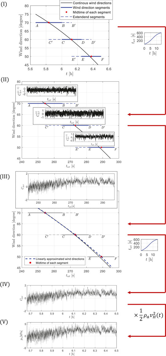
FIGURE 1. Conceptual flowchart of the non-stationary/-straight/-Gaussian stochastic wind pressure simulation model.

4.1.2 Procedure

In the following, further details of each step of the model outlined in Figure 1 are provided.

Step I

The continuous wind direction history, α_H(t), is first discretized into a set of segments with each segment representing a straight wind event. This discretization can be expressed as:

${\bar{\alpha }}_H\left(t\right)=\mathrm{n}\mathrm{i}\mathrm{n}\mathrm{t}\left(\frac{{\alpha }_H\left(t\right)}{\mathrm{\Delta }\alpha }\right)\mathrm{\Delta }\alpha (16)$

where ${\bar{\alpha }}_H(t)$ is the discretized wind direction history, nint is the function which returns a number rounded to the nearest integer, Δα is the direction step size of the wind tunnel data (e.g., Δα = 10°). Each segment, ${\bar{\alpha }}_H^{(i)}(t)$, represents a straight wind event, where i ∈ {1, 2, …, N_seg} with N_seg the total number of segments defining ${\bar{\alpha }}_H(t)$. Within the segment ${\bar{\alpha }}_H^{(i)}(t)$, the mid-time is denoted by $T_m^{(i)}$ (e.g., the red dots in Figure 1) with the start and end time denoted by $T_s^{(i)}$ and $T_e^{(i)}$. To form the transition region, each segment is further extended on both ends up to the mid-times of the nearby segments (i.e., the ith segment is extended to $T_m^{(i-1)}$ and $T_m^{(i+1)}$ with the boundary cases of i = 1 and i = N_seg treated by only extending one end).

Step II

In this step, a wind pressure coefficient vector process, ${\mathbf{C}}_{p,e,M}^{(i)}(t_M)$, is generated for each extended segment at the model-scale. To obtain the total duration of each extended segment at model-scale, the following nonlinear time-scale mapping from t to t_M is derived based on Strouhal number matching:

$t_M\left(t\right)=\frac{{\gamma }_H}{{\bar{v}}_M}{\int }_0^t{\bar{v}}_H\left(u\right)du(17)$

where γ_H is the ratio of the model to full-scale height and ${\bar{v}}_M$ is the mean wind speed used during the wind tunnel tests. Based on Eq. 17, the duration of the ith extended segment can be calculated from:

$T_{seg}^{\left(i\right)}=\left\{\begin{array}{c}{t}_M\left(T_m^{\left(i+1\right)}\right)-t_M\left(T_s^{\left(i\right)}\right)\text{\hspace{0.17em}if\hspace{0.17em}}i=1\hfill \\ t_M\left(T_e^{\left(i\right)}\right)-t_M\left(T_m^{\left(i-1\right)}\right)\text{\hspace{0.17em}if\hspace{0.17em}}i=N_{seg}\hfill \\ t_M\left(T_m^{\left(i+1\right)}\right)-t_M\left(T_m^{\left(i-1\right)}\right)\text{\hspace{0.17em}otherwise\hspace{0.17em}}\hfill \end{array}\right.(18)$

where $T_{seg}^{(i)}$ is the duration of the ith extended segment.

Through Eq. 18, the duration of each extended segment is calculated and used to simulate the stationary/straight but non-Gaussian wind pressure coefficient vector processes, ${\mathbf{C}}_{p,e,M}^{(i)}(t_M)$, through the models outlined by Ouyang and Spence (2020). The maximum possible sampling frequency (dictated by the wind tunnel data) should be chosen in generating ${\mathbf{C}}_{p,e,M}^{(i)}(t_M)$ to minimize any interpolation errors in Step (V).

Step III

From the stationary wind pressure coefficient vector processes ${\mathbf{C}}_{p,e,M}^{(i)}(t_M)$ of step (II), a filter-based transition model is introduced to merge the segments into a non-stationary/-straight/-Gaussian wind pressure coefficient vector process C_p,e,M(t_M). To implement the transition, the stationary processes ${\mathbf{C}}_{p,e,M}^{(i)}(t_M)$ are decomposed into a time-averaged component, ${\bar{\mathbf{C}}}_{p,e,M}^{(i)}(t_M)$, and a fluctuation component, ${\tilde{\mathbf{C}}}_{p,e,M}^{(i)}(t_M)$, such that:

${\mathbf{C}}_{p,e,M}^{\left(i\right)}\left(t_M\right)={\bar{\mathbf{C}}}_{p,e,M}^{\left(i\right)}\left(t_M\right)+{\tilde{\mathbf{C}}}_{p,e,M}^{\left(i\right)}\left(t_M\right)(19)$

The following linear ramping-based filter is then applied to each time-averaged component:

${\psi }^{\left(i\right)}\left(t_M\right)=\left\{\begin{array}{c}1‐\frac{t_M-T_{M,m}^{\left(i\right)}}{T_{M,m}^{\left(i+1\right)}-T_{M,m}^{\left(i\right)}}\text{\hspace{0.17em}if\hspace{0.17em}}{t}_M>T_{M,m}^{\left(i\right)}\hfill \\ 1‐\frac{T_{M,m}^{\left(i\right)}-t_M}{T_{M,m}^{\left(i\right)}-T_{M,m}^{\left(i-1\right)}}\text{\hspace{0.17em}if\hspace{0.17em}}{t}_M\le T_{M,m}^{\left(i\right)}\hfill \end{array}\right.(20)$

where $T_{M,m}^{(i)}$ is the mid-time of the ith segment in model-scale time. Based on this linear filter, the merged time-averaged components, with $t_M\in [T_{M,m}^{(i)},T_{M,m}^{(i+1)}]$, are defined as:

${\bar{\mathbf{C}}}_{p,e,M}\left(t_M\right)={\psi }^{\left(i\right)}\left(t_M\right){\bar{\mathbf{C}}}_{p,e,M}^{\left(i\right)}\left(t_M\right)+{\psi }^{\left(i+1\right)}\left(t_M\right){\bar{\mathbf{C}}}_{p,e,M}^{\left(i+1\right)}\left(t_M\right)(21)$

To merge the fluctuation components, ${\tilde{\mathbf{C}}}_{p,e,M}^{(i)}(t_M)$, a nonlinear ramping-based filter in the form of the square root of ψ⁽ⁱ⁾ is applied, with $t_M\in [T_{M,m}^{(i)},T_{M,m}^{(i+1)}]$, as follows:

${\tilde{\mathbf{C}}}_{p,e,M}\left(t_M\right)=\sqrt{{\psi }^{\left(i\right)}\left(t_M\right)}{\tilde{\mathbf{C}}}_{p,e,M}^{\left(i\right)}\left(t_M\right)+\sqrt{{\psi }^{\left(i+1\right)}\left(t_M\right)}{\tilde{\mathbf{C}}}_{p,e,M}^{\left(i+1\right)}\left(t_M\right)(22)$

By iterating over all segments, with special boundary consideration for i = 1 and i = N_seq, ${\bar{\mathbf{C}}}_{p,e,M}(t_M)$ and ${\tilde{\mathbf{C}}}_{p,e,M}(t_M)$ are estimated for the entire hurricane track. The final non-stationary/-straight/-Gaussian wind pressure coefficient vector process is then obtained as:

${\mathbf{C}}_{p,e,M}\left(t_M\right)={\bar{\mathbf{C}}}_{p,e,M}\left(t_M\right)+{\tilde{\mathbf{C}}}_{p,e,M}\left(t_M\right)(23)$

Through the transition model outlined above, the merged wind pressure vector process will have second-order statistics (auto- and cross-correlation functions) that vary following a near-linear relationship between the wind directions in which wind tunnel data are available. Inherent to this transition model is the capture of non-Gaussianity in C_p,e,M(t_M) that matches those observed in the wind tunnel for the discrete wind directions at which wind tunnel tests were performed.

Step IV

To generate the wind pressure vector process at a building-scale with a target constant sampling frequency, the model-scale wind pressure coefficient vector process needs to be sampled with a nonuniform sampling frequency due to the continuously varying wind speed –v_H(t). This nonuniform sampling is achieved through a model-scale interpolation scheme, where the uniform time samples t_l, with l ∈ (1, 2, …, N_l) and N_l the total number of uniform samples at a building-scale, are mapped to the model-scale through Eq. 17. This leads to a nonuniform space of model-scale time samples t_M(t_l) that are evaluated through interpolation. The discrete representation of the building-scale non-stationary/-straight/-Gaussian pressure coefficient vector process, C_p,e(t_l), is defined as:

${\mathbf{C}}_{p,e}\left(t_l\right)={\mathbf{C}}_{p,e,M}\left(t_M\left(t_l\right)\right)(24)$

Step V

From the pressure coefficient processes of Eq. 24, the non-stationary/-straight/-Gaussian external pressures can be estimated as:

${\mathbf{p}}_e\left(t_l\right)=\frac{1}{2}{\rho }_a{v_H}^2\left(t_l\right){\mathbf{C}}_{p,e}\left(t_l\right)(25)$

where p_e is the vector of the non-stationary/-straight/-Gaussian pressure processes at the sensor grid locations at full scale. To estimate the pressure processes at a location, identified by the coordinate ξ_xyz, on the building envelope where direct measurements were not carried out, 2D interpolation with extrapolation can be used (Ouyang and Spence, 2019, 2020).

4.2 Wind-driven Rain

The simulation of the time-dependent wind-driven rain is developed through the extension of the nominal wind-driven rain model outlined by Ouyang and Spence (2020). For the nominal hurricane, constant wind-driven rain is simulated through the 3D steady Reyolds-averaged Navier-Stokes (RANS) equations-based Eulerian multiphase (EM) model proposed by (Huang and Li (2012); Kubilay et al., (2013, 2017). The implementation of this framework consists of two steps: 1) the RANS equations with a realizable k-ϵ turbulence model are solved for the steady-state wind field around the building; and 2) based on the steady-state solution from the first step, the EM model is implemented with the k − ϵ turbulence model to solve for wind-dispersed rain phases. In particular, each rain phase represents a phase flow problem for a group of raindrops with diameters in a predefined range. The solution of the EM model gives a vector of normalized specific catch ratios, $\bar{\mathit{\eta }}({\xi }_{xyz})$, for all rain phases at each location, ξ_xyz, of interest. The corresponding wind-driven rain can then be directly calculated based on the rainfall intensity, R_h, and the associated conditional raindrop diameter distribution.

To model the time-dependency of the wind-driven rain due to the continuously varying wind speed and direction, the specific catch ratios would need to be continuously solved in time. This poses a significant computational issue as this would in general imply the need to solve RANS-based EM models for a sequence of wind speeds and directions for each storm track of interest. To overcome this issue, an interpolation-based approach is adopted, where the specific catch ratios at each envelope point of interest, $\bar{\mathit{\eta }}({\xi }_{xyz})$, are pre-computed for a predetermined grid of wind directions and wind speeds. The time-dependency of $\bar{\mathit{\eta }}({\xi }_{xyz})$ can then be efficiently estimated through instantaneous interpolation at α_H(t) and v̄_H(t). Based on this approach, the time-dependent wind-driven rain intensity at each envelope location of interest, R_wdr(ξ_xyz, t), is estimated as:

$R_{wdr}\left({\xi }_{xyz},t\right)={\mathrm{\Phi }}^T\left(t\right)\bar{\mathit{\eta }}\left({\xi }_{xyz},{\alpha }_H\left(t\right),{\bar{v}}_H\left(t\right)\right)(26)$

where Φ(t) is a weighting vector whose kth component is defined as:

${\mathrm{\Phi }}_k\left(t\right)=R_h\left(t\right)\mathrm{\Delta }{d}_k{f}_h\left(d_k|R_h\left(t\right)\right)(27)$

where Δd_k is the raindrop diameter range of the kth rain phase, d_k is the median raindrop diameter in the kth rain phase, and f_h is the PDF of the raindrop diameter distribution.

5 Response Analysis: System Analysis

Based on the envelope actions, demands in terms of dynamic story drifts and local net dynamic pressures can be estimated through the adoption of the models outlined by Ouyang and Spence (2020). Based on these demands, system measures, sm, associated with the final damage states of each vulnerable envelope component and subsequent water ingress can be evaluated. As will be briefly outlined below, the use of the models outlined by Ouyang and Spence (2020) enables not only the capture of the interdependencies between demands and damages but also the progressive nature of wind-induced damage.

5.1 Demands

5.1.1 Structural Response

Based on the results reported by Ouyang and Spence (2021), the structural system is assumed to respond elastically. The dynamic response of the structural system can therefore be estimated through solving the following modal equations:

${\ddot{q}}_i\left(t\right)+2{\omega }_i{\zeta }_i{\dot{q}}_i\left(t\right)+{\omega }_i^2{q}_i\left(t\right)=Q_i^{\mathcal{N}}\left(t\right)(28)$

where q_i, ${\dot{q}}_i$, and ${\ddot{q}}_i$ are the displacement, velocity, and acceleration associated with the ith dynamic mode; ω_i and ζ_i are the circular frequency and modal damping ratio of the ith mode, while $Q_i^{\mathcal{N}}(t)$ is the non-stationary/-straight/-Gaussian generalized force of the ith mode estimated as:

$Q_i^{\mathcal{N}}\left(t\right)=\frac{{\varphi }_i^T}{{\varphi }_i^T\mathbf{M}{\varphi }_i}{\tilde{\mathbf{f}}}_{\mathcal{N}}\left(t\right)(29)$

where ϕ_i is the ith mode shape; M is the structural mass matrix; and ${\tilde{\mathbf{f}}}_{\mathcal{N}}(t)$ is the dynamic forcing vector evaluated through integrating the non-stationary/-straight/-Gaussian pressures of Eq. 25.

From the solution of Eq. 28, the dynamic structural response can be approximated from the first N_m modes as:

$\mathbf{x}\left(t\right)\approx \sum _{i=1}^{N_m}{\varphi }_i{q}_i\left(t\right)(30)$

Dynamic story drift, Dr(t), at any location of interest can then be directly estimated through a linear combination of the appropriate components of x(t).

5.1.2 Net Dynamic Pressure

The net pressure demands at an envelope location ξ_xyz of interest, p_n(t, ξ_xyz), are evaluated as:

$p_n\left(t,{\xi }_{xyz}\right)=p_e\left(t,{\xi }_{xyz}\right)-p_i\left(t,{\xi }_{xyz}\right)(31)$

where _e(t, ξ_xyz) is the external pressure estimated through the models of Section 4.1 at ξ_xyz while p_i(t, ξ_xyz) is the corresponding internal pressures. To estimate the dynamic internal pressures p_i(t, ξ_xyz), the interior of the building is modeled as a system of interconnected compartments. Initially, the building is considered enclosed with negligible internal pressurization. During the hurricane, openings can be created in the envelope due to component damages, which allows air to flow into or out of the building triggering dynamic internal pressures in all compartments that are connected through an internal opening. To solve the transient air flows, the internal pressure model outlined by Ouyang and Spence (2019) is adopted, in which the air velocity at each opening is described through the unsteady-isentropic form of the Bernoulli equation (Vickery and Bloxham, 1992; Yu et al., 2008; Guha et al., 2011). To treat the time dependency of ${\bar{v}}_H$, the dynamic internal pressures, p_i(t, ξ_xyz), at each opening (external/internal or internal/internal), are directly estimated through solving a system of nonlinear equations (one for each opening) derived based on the principle of mass conservation. A fourth-order Runge Kutta scheme can be used to solve the system where, at each time step, the pressure-induced damages are iteratively updated until dynamic equilibrium is achieved.

It is important to observe that in solving for p_i(t, ξ_xyz), the current drift-induced damage state of each envelope component must be considered. This couples not only the structural and pressure demands (e.g., a drift-induced damage to the envelope can cause air flow therefore affecting the internal pressure) but also the demand and damage analysis (e.g., the occurrence of a drift- or pressure-induced damage state can affect internal pressures). It should also be observed that damage to the envelope is progressive in nature as it accumulates over the duration of the event.

5.2 System Measures

5.2.1 Component Damages

To model the damage susceptibility of the ith envelope component to $N_{Dr}^i$ drift-induced and $N_P^i$ pressure-induced damage states, suites of $N_{Dr}^i$ and $N_P^i$ sequential damage thresholds are defined: ${\mathbf{C}}_P^i=\{C_{P_1}^i\le C_{P_2}^i\dots ,\le C_{P_{N_P}}^i\}$ and ${\mathbf{C}}_{Dr}^i=\{C_{D{r}_1}^i\le C_{D{r}_2}^i\dots ,\le C_{D{r}_{N_{Dr}}}^i\}$. The randomness in the thresholds is modeled through corresponding suites of sequential fragility functions. At a given time step, $\widehat{t}$, all component thresholds are compared with the current story drift demand, $D{r}^i(\widehat{t})$, and net pressure demand $p_n(\widehat{t},{\xi }_{xyz}^i)$, where the largest exceeded threshold defines the current pressure- and/or drift-induced damage state. To model potential coupling between drift- and pressure-induced damage states (e.g., the occurrence of a drift-induced damage state could affect the capacity of the component to resist net pressure and vice versa), the thresholds of a suite of coupled damage states are probabilistically degenerated upon the occurrence of the coupled damage state. The final damage states of each envelope component represent the system measures of interest.

5.2.2 Water Ingress

The concurrent rainfall leads to the deposition of rainwater on the envelope. Damage to the envelope can then lead to water ingress. To estimate the volume of water ingress, the flow rate at each opening can be estimated directly from R_wdr(ξ_xyz, t), estimated through the models of Section 4.2, and the steady-state water runoff solution derived by Ouyang and Spence (2019). From the flow rate at each opening, the total volume of water entering through an opening at a given time, $\widehat{t}$, can be estimated by integrating the flow rate from the time the opening first occurred, i.e., the time at which the damage causing the opening occurred. Through the implementation of the water ingress model, the time traces of total volume of water entering through each opening can be estimated.

6 Loss and Consequence Analysis

To translate the final damage states of each envelope component into repair costs and actions, the concept of unit loss function (ULF), as defined by Federal Emergency Management Agency (FEMA) (2012), is adopted. Specifically, the ULF defines the repair cost as a monotonically decreasing function with respect to the total number of components in a given damage state. To consider economies of scale, a minimum quantity, Q_min, is defined as the lower limit below which economies of scale do not take effect. Likewise, a maximum quantity, Q_max, is defined as the upper limit after which economies of scale no longer occur. To include uncertainty in the loss estimation, the value given by the ULF is taken as the expected value of a lognormal random variable with assigned dispersion. This dispersion accounts, to a certain extent, for the many complexities involved in estimating repair cost and time following a hurricane, e.g., administrative backlogs, demand surge, lack of materials, and shortage of labor. Through ULFs, each envelope damage state can be converted to estimates of the repair cost (or time). The evaluation of the total system level repair cost, i.e., the decision variable (dv), can then be evaluated by summing all envelope component repair costs. This scheme can also be used to estimate downtimes associated with repair actions. Similarly, the system-level consequence of envelope damage related to total volume of water ingress can be assessed by summing the volumes of water ingress at each damaged envelope component. Additionally, the information provided by the framework on water ingress would support the use of models for estimating damage to the interior components and contents by providing detailed information on the water paths and flow rates at each damaged envelope component.

7 Simulation Strategy

The evaluation of the envelope system performance relies on the possibility of efficiently solving Eq. 3. Because the failure rates of interest to this work are small, i.e., related to rare events, and the models used to characterize performance are computational intense, direct Monte Carlo (MC) methods are generally intractable. To overcome this, a conditional stochastic simulation scheme that integrates subset simulation (Au and Beck, 2001) is developed. The approach is based on using ${\bar{v}}_H$ as an indicator of hurricane intensity. The hazard curve is then divided into $N_{{\bar{v}}_H}$ mutually exclusive and collectively exhaustive hazard intervals with each interval representing a set of sub-events of intensity measured over intervals of maximum mean hourly wind speed. The performance within each sub-event is evaluated using direct MC methods. The samples for each sub-event are generated through a hybrid simulation technique in which hurricane track samples, i.e., realizations of Θ conditional on the sub-event, are efficiently generated through Markov chain Monte Carlo (MCMC) algorithms and combined with randomly sampled sets of model parameters (e.g., the component thresholds and modal damping ratios). Following this strategy, Eq. 3 is reformulated through the total probability theorem as:

$\lambda \left(dv\right)={\lambda }_e\sum _{k=1}^{N_{{\bar{v}}_H}}\left[\iint G\left(dv|sm\right)|dG\left(sm|\mathbf{\Theta }\right)\Vert dG\left(\mathbf{\Theta }|E_{{\bar{v}}_H,k}\right)|\right]P\left(E_{{\bar{v}}_H,k}\right)(32)$

where $E_{{\bar{v}}_H,k}$ is the kth sub-event defined as ${\bar{v}}_H\in [{\bar{v}}_{H,k}^L,{\bar{v}}_{H,k}^U)$ with ${\bar{v}}_{H,k}^L$ and ${\bar{v}}_{H,k}^U$, the lower- and upper-bound wind speed defining the kth interval, where ${\bar{v}}_{H,k}^U=+\infty$ for $k=N_{{\bar{v}}_H}$; $P(E_{{\bar{v}}_H,k})$ is the probability of a hurricane sample belonging to $E_{{\bar{v}}_H,k}$ (which can be directly estimated from the hazard curve); $N_{{\bar{v}}_H}$ is the total number of sub-events; and λ_e is the annual recurrence rate of hurricanes of engineering interest.

To evaluate Eq. 32 through the approach outlined above, subset simulation is first used to estimate the hazard curve, $\lambda ({\bar{v}}_H)$, through sampling the space of Θ while using ${\bar{v}}_H$ as the response of interest. In particular, it is convenient to select the lower and upper bound wind speeds for each sub-event based on the thresholds of ${\bar{v}}_H$ identified during the implementation of subset simulation. In this way, the number of intervals will depend on the target exceedance probability set for the lower bound of the last interval and the intermediate probability, P_s, used in calibrating the subset simulation algorithm. Furthermore, the probabilities $P(E_{{\bar{v}}_H,k})$ can be directly estimated from P_s. The number of samples used for each conditional failure event of the subset simulation will dictate the maximum number of samples that can be used to evaluate the term in square brackets of Eq. 32 through MC simulation. Therefore, the number of samples should be chosen to provide adequate resolution.

8 Case Study

8.1 Building System

To illustrate the proposed framework while also studying the differences between performance assessments carried out using nominal as opposed to full hurricane hazard models, the archetype building outlined in (Ouyang and Spence, 2020) with location Miami, FL, is considered. As shown in Figure 2, the building is a rectangular 45-story steel structure with central core and symmetric X-bracing. The total height of the structure is 180 m with a constant floor height of 4 m. The structural system was designed to satisfy typical serviceability and life safety requirements. The first 10 vibration modes were considered adequate for representing the dynamic response. The first three natural frequencies were 1.30, 1.67, and 2.70 rad/s, respectively. The damageable components considered in the case study are the dual-pane laminated glazing units of size of 1.2 × 2 m². The thickness of each laminated pane is taken as 6 mm. Each floor has 180 units with 60 units on the south (north) face and 30 units on the east (west) face, which results in a total of 8,100 units for the entire building. To calibrate the damage model of Section 5.2.1, two drift-induced damages states (defined as hairline cracking, $D{S}_{D{r}_1}$, and the glass cracking, $D{S}_{D{r}_2}$) and one pressure-induced damage state $D{S}_{P_{60}}$ (defined as full loss of the window panes) are defined with random thresholds calibrated through the fragility functions reported in Table 1. The dual panes are considered fully correlated in terms of capacity and to work in parallel when resisting net pressure, modeled as equivalent over a duration of 60 s (Ouyang and Spence, 2020). Further details on the case study building, including the pre-computed wind-driven rain simulations for calibrating Eq. 26, can be found in Appendix.

FIGURE 2

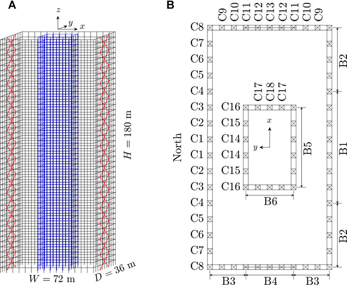
FIGURE 2. (A) Three-dimensional illustration of the 45-story structure; (B) plan view indicating the floor member layout (B = beam and C = column) and North.

TABLE 1

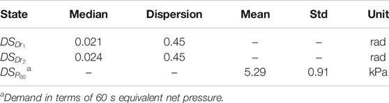
TABLE 1. Fragility functions for each glazing unit.

8.2 Hurricane Hazard

To calibrate the parametric hurricane model of Section 3.2.1, and therefore the vector Θ to Miami, a subregion diameter of R_s = 500 km was considered while the probabilistic characteristics of the components of Θ followed those suggested by Vickery and Twisdale (1995a). In converting mean hourly wind speeds at 500 m to H = 180 m (i.e., building top) through Eq. 10, values of z₀ = 1.28 m and z₀₁ = 0.03 m were considered. The aerodynamic model of Section 4.1.2 was calibrated to a data set of the Tokyo Polytechnic University (TPU) wind tunnel pressure database (Tokyo Polytechnic University, 2008). These data are used to calibrate the stationary/straight but non-Gaussian wind pressure coefficient processes, C_p,e,M(t_M), at model-scale. For the data set considered, the ratio of tunnel model height to building height, γ_H, was 1:360 while the mean wind speed at model height during the wind tunnel tests was ${\bar{v}}_M=11.11$ m/s. The turbulence intensity was 25% while the wind speed profile had a power-law coefficient of 1/4. During the tests, transient pressure coefficients were simultaneously measured at 510 pressure taps located over the building surface with a constant sampling frequency of 1,000 Hz and a wind direction increment of 10°. Based on C_p,e,M(t_M), realizations of the non-stationary/-straight/-Gaussian wind pressure vector process, C_p,e(t), were generated through the five-step procedure of Section 4.1.2.

As defined in Section 3.2.1, each sample of Θ uniquely determines the hurricane track of a full hurricane. To estimate the hazard curve through subset simulation, an intermediate probability of P_s = 0.2 was chosen together with $N_{{\bar{v}}_H}=9$ conditional failure events. Considering how λ_e = 1.22 for Miami (Vickery and Twisdale, 1995a), this leads to a lower bound wind speed with an annual exceedance rate of ${\lambda }_e{(P_s)}^8=3.123\times 10^{-6}$, i.e., a mean recurrence interval of over 300,000 years, which is considered adequate for evaluating the performance of the system for PBWE design scenarios. Within each subset, N_s = 1,300 samples of Θ are considered. In running the MCMC Metropolis Hasting algorithm, a univariate normal distribution with zero mean and standard deviation of 0.5 was considered as the proposal pdf. The choice of N_s = 1,300 leads to N_s(1 − P_s) = 1,040 hurricane samples for the subsequent MC analysis necessary for evaluating Eq. 32 through the procedure of Section 7. The final hazard curve is reported in Figure 3.

FIGURE 3

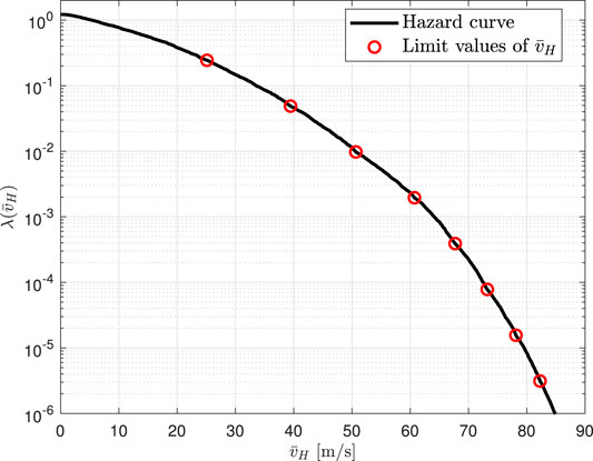
FIGURE 3. The estimated hurricane hazard curve.

8.3 Results

8.3.1 Preamble

To enable the comparison between the full hurricane model of this work and a classic nominal hurricane setting, for each full hurricane sample, a nominal hurricane is also generated based on the maximum wind speed ${\bar{v}}_H$, with associated direction α_H, and the maximum rainfall intensity to occur over the duration of the full hurricane. For both nominal and full hurricanes, a uniform time step of Δt = 0.5 s at building-scale is used.

8.3.2 Discussion on a Single Event

To illustrate and discuss the evolution of damage during a full hurricane event, a single hurricane event is analyzed in detail in this section. The event corresponds to a category five hurricane on the Saffir-Simpson scale (Taylor et al., 2010), with a maximum mean hourly wind speed at the building top of 67.7 m/s. The time evolution of mean hourly wind speed ${\bar{v}}_H(t)$, wind direction α_H(t) (measured counterclockwise from south), and mean hourly rainfall intensity R_h(t) is reported in Figure 4. An example of the corresponding non-stationary/-straight/-Gaussian wind pressure simulated through the procedure of Section 4.1 is shown in Figure 5 for an envelope component located at the upper-left corner of the south face of the building.

FIGURE 4

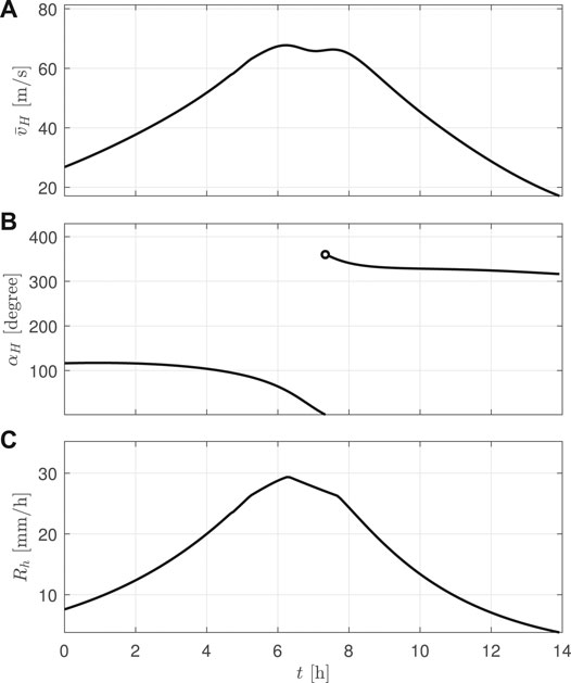
FIGURE 4. The simulated category V hurricane in Saffir-Simpson scale measured at the building site: (A) evolution of the mean hourly wind speed; (B) wind direction; and (C) mean hourly rainfall intensity.

FIGURE 5

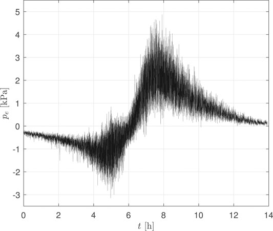
FIGURE 5. An example of the non-stationary/-straight/-Gaussian external wind pressure process for an envelope component located at the upper-left corner of the south face of the building.

Figure 6 reports the accumulation of damage over the duration of the hurricane in terms of the total number of envelope components assuming $D{S}_{D{r}_1}$, $D{S}_{D{r}_2}$, or $D{S}_{P_{60}}$. From the comparison between the damage histories and the wind speed history of Figure 4A, it can be seen that most damage occurs near the time of the maximum wind speed, i.e., during the 7th hour of the hurricane event. By the end of the hurricane event, the final damage states for each envelope component were recorded and are reported in Table 2 in terms of the number of damaged components on each face of the building. As can been seen, due to the continuously varying wind direction, the damage is relatively evenly distributed between the faces. The distribution of final damages shows how pressure-induced damages are dominant, which is consistent with the results reported by Ouyang and Spence (2020) for a nominal hurricane representation. Water ingress is also recorded during and at the end of the hurricane, where a total volume of 270.5 m³ of water was estimated to enter the building through the damaged envelope components. The time histories of water ingress at each floor during the hurricane are reported in Figure 7 and show how water ingress towards the bottom of the building dominates.

FIGURE 6

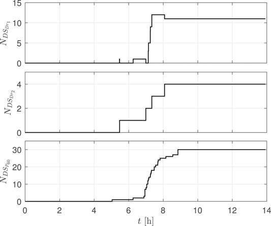
FIGURE 6. Time histories of the total number of components in damage states $D{S}_{D{r}_1}$, $D{S}_{D{r}_2}$, and $D{S}_{P_{60}}$.

TABLE 2

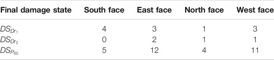
TABLE 2. Number of envelope components assuming $D{S}_{D{r}_1}$, $D{S}_{D{r}_2}$, or $D{S}_{P_{60}}$ as final damage state.

FIGURE 7

FIGURE 7. Time histories of the water ingress at each floor.

8.3.3 Probabilistic Performance Metrics

The mean annual rate of each envelope component assuming as a final damage state $D{S}_{D{r}_1}$, $D{S}_{D{r}_2}$, or $D{S}_{P_{60}}$ is reported in Figure 8. The damage maps show how the drift-induced damages are uniformly distributed over the envelope except for the top and bottom floors, while the pressure-induced damages are more concentrated near the edges of the building due to the local aerodynamic response of the system. Overall, the damage patterns and rates are similar to those seen for the nominal hurricane setting analyzed by Ouyang and Spence (2020).

FIGURE 8

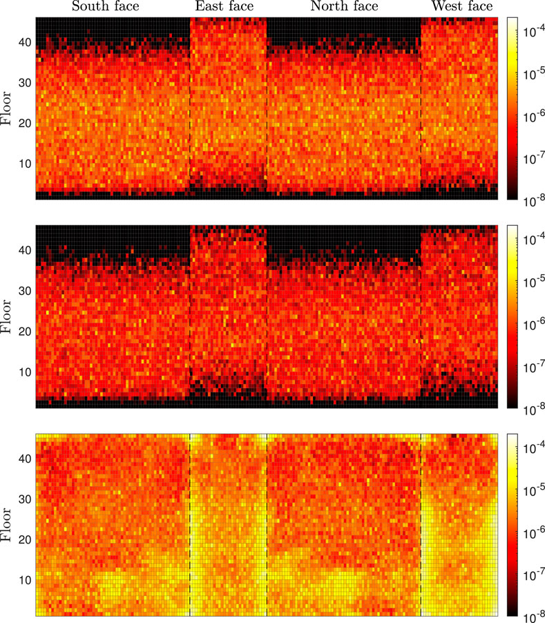
FIGURE 8. Mean annual rate of each envelope component assuming as a final damage state $D{S}_{D{r}_1}$, $D{S}_{D{r}_2}$, or $D{S}_{P_{60}}$. Top panel is associated with $D{S}_{D{r}_1}$, middle panel with $D{S}_{D{r}_2}$, and bottom panel with $D{S}_{P_{60}}$.

To evaluate the system-level envelope performance for both the nominal and full hurricanes, Figure 9 reports the damage curves for both scenarios in terms of the mean annual rate of exceeding a total number of components assuming as a final damage state $D{S}_{D{r}_1}$, $D{S}_{D{r}_2}$, or $D{S}_{P_{60}}$. Comparison between the drift-induced damage curves shows how the total number of damaged components is well estimated by the nominal hurricane for annual rates greater than 2 × 10^–6. However, for rarer events, the nominal hurricane will generally lead to considerable overestimation of damage. For pressure-induced damage, it can be seen that the nominal hurricanes underestimate the damages for mean annual rates greater than 2 × 10^–6, but once again significantly overestimate the damages for rarer events. The differences in Figure 9 are likely caused by the duration of the maximum wind T_m, where T_m is defined as the duration when the hurricane wind speed ${\bar{v}}_H(t)$ is within a certain percentage of the maximum wind speed ${\widehat{\bar{v}}}_H=\text{max}[{\bar{v}}_H(t)]$ (e.g., ${\bar{v}}_H(t)\ge 0.95{\widehat{\bar{v}}}_H$). Indeed, the storm track model considered in this study suggests that hurricanes with a larger maximum mean wind speed, ${\widehat{\bar{v}}}_H$, have a relatively “sharper” wind speed history curve (i.e., the duration of the maximum wind is shorter).

FIGURE 9

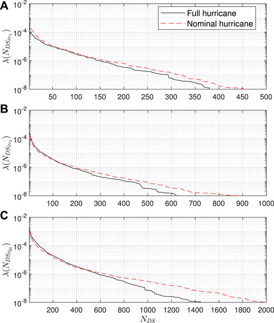
FIGURE 9. Mean annual rate of exceeding a total number of envelope components assuming as a final damage state: (A) $D{S}_{D{r}_1}$; (B) $D{S}_{D{r}_2}$; (C) $D{S}_{P_{60}}$.

To investigate this, the distribution of maximum wind speed duration is analyzed for all hurricane samples in hazard intervals three to nine, where the first two intervals are not considered as the value of ${\widehat{\bar{v}}}_H$ is negligible from an engineering standpoint. The mean and standard deviation of the durations are reported in Figure 10, from which it can be seen that as the hurricane event becomes rarer, the duration of maximum wind becomes shorter. In particular, it can be seen that wind speeds within 98% of the maximum have an expected duration of around one-hour duration. The capability of the nominal hurricane to adequately reproduce the damage would suggest that envelope damage is occurring essentially when wind speeds are at their maximum.

FIGURE 10

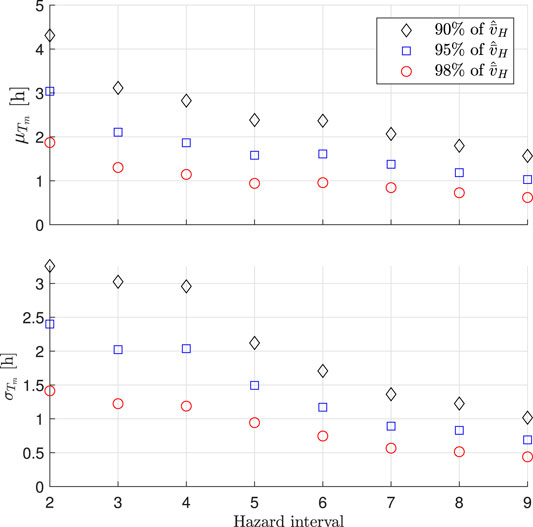
FIGURE 10. Mean, ${\mu }_{T_m}$, and the standard deviation, ${\sigma }_{T_m}$, of T_m for hazard intensity intervals three to nine.

The loss curves associated with repair costs are reported in Figure 11. The relative magnitude of total repair cost between the nominal and full hurricanes is similar to the damage curves of Figure 9C, which implies that the pressure-induced damages dominate the total repair cost associated with the envelope components. Figure 12 reports the exceedance rates associated with the consequence metric of total volume of water ingress V_W. From the comparison of the water ingress curves, the nominal hurricane significantly underestimates the total amount of water ingress as compared to the full hurricane. To quantify this underestimation, Table 3 reports the total water ingress at different exceedance rates for the nominal and full hurricanes. As can be seen, a near 40-fold underestimation of water ingress can be seen for exceedance rates of 1 × 10^–3. The root of this difference can be traced back to how the nominal hurricane neglects the water that can enter the building due to rainfall after the peak wind speeds have occurred. As the exceedance rates decrease, the underestimation of total water ingress from the nominal hurricane also decreases. This is due to how as the hurricane events become more extreme, the majority of damage will occur at the beginning of the nominal hurricane event therefore increasing the duration in which water can ingress.

FIGURE 11

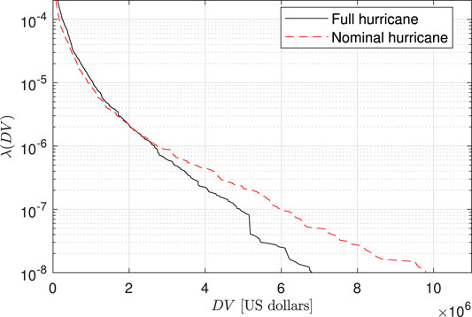
FIGURE 11. Repair cost loss curves in United States dollars for the nominal and full hurricanes.

FIGURE 12

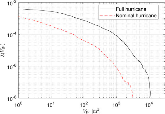
FIGURE 12. Consequence curve associated with total water ingress due to envelope damage.

TABLE 3

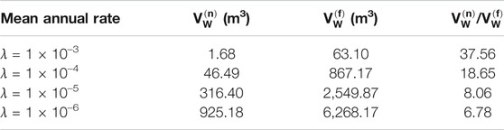
TABLE 3. Comparison between total water ingress in the nominal hurricane ($V_W^{(n)}$) and full hurricane ($V_W^{(f)}$).

9 Summary and Conclusion

A framework is outlined for the performance assessment of the envelope system of engineered buildings subject to a full representation of the hurricane hazard. A new wind-tunnel-informed non-stationary/-straight/-Gaussian wind pressure stochastic simulation model is introduced to support full hurricane event simulation. Through the development of a conditional stochastic simulation framework, efficient estimation of probabilistic metrics associated with the performance of the envelope system in rare events is made possible. The framework was illustrated through a case study consisting of a 45-story archetype building located in Miami, FL. Performance metrics associated with the total number of damaged envelope components, monetary loss, and total water ingress were evaluated. The comparison of the performance metrics with those estimated for a classic nominal representation of the hurricane hazard showed that performance assessments made with the nominal hurricane representation will generate similar amounts of damages and losses for a mean annual rate greater than 2 × 10^–6. For events with smaller rates than 2 × 10^–6, the nominal hurricanes significantly overestimated (up to 50%) the damages and losses. In terms of the water ingress, a full hurricane representation will generate a much larger volume of water ingress, over 30-fold larger for rates of 1 × 10^–3, than seen for simulations using a nominal hurricane representation. This underestimation was seen to decrease with the reduction of the exceedance rates.

Data Availability Statement

The original contributions presented in the study are included in the article/Supplementary Material, and further inquiries can be directed to the corresponding author.

Author Contributions

All authors listed have made a substantial, direct, and intellectual contribution to the work and approved it for publication.

Funding

The research effort was supported in part by the United States (US) National Science Foundation (NSF) under Grant No. CMMI-1562388 and CMMI-1750339. This support is gratefully acknowledged.

Conflict of Interest

The authors declare that the research was conducted in the absence of any commercial or financial relationships that could be construed as a potential conflict of interest.

Publisher’s Note

All claims expressed in this article are solely those of the authors and do not necessarily represent those of their affiliated organizations, or those of the publisher, the editors and the reviewers. Any product that may be evaluated in this article, or claim that may be made by its manufacturer, is not guaranteed or endorsed by the publisher.

References

Au, S.-K., and Beck, J. L. (2001). Estimation of Small Failure Probabilities in High Dimensions by Subset Simulation. Probabilistic Eng. Mech. 16, 263–277. doi:10.1016/s0266-8920(01)00019-4

CrossRef Full Text | Google Scholar

Barbato, M., Petrini, F., Unnikrishnan, V. U., and Ciampoli, M. (2013). Performance-based hurricane Engineering (PBHE) Framework. Struct. Saf. 45, 24–35. doi:10.1016/j.strusafe.2013.07.002

CrossRef Full Text | Google Scholar

Bernardini, E., Spence, S. M. J., Kwon, D.-K., and Kareem, A. (2015). Performance-based Design of High-Rise Buildings for Occupant comfort. J. Struct. Eng. 141, 1–14. doi:10.1061/(asce)st.1943-541x.0001223

CrossRef Full Text | Google Scholar

Brackins, J. T., and Kalyanapu, A. J. (2020). Evaluation of Parametric Precipitation Models in Reproducing Tropical Cyclone Rainfall Patterns. J. Hydrol. 580, 124255. doi:10.1016/j.jhydrol.2019.124255

CrossRef Full Text | Google Scholar

Chen, S. S., Knaff, J. A., and Marks, F. D. (2006). Effects of Vertical Wind Shear and Storm Motion on Tropical Cyclone Rainfall Asymmetries Deduced from TRMM. Monthly Weather Rev. 134, 3190–3208. doi:10.1175/mwr3245.1

CrossRef Full Text | Google Scholar

Chuang, W.-C., and Spence, S. M. J. (2017). A Performance-Based Design Framework for the Integrated Collapse and Non-collapse Assessment of Wind Excited Buildings. Eng. Structures 150, 746–758. doi:10.1016/j.engstruct.2017.07.030

CrossRef Full Text | Google Scholar

Ciampoli, M., Petrini, F., and Augusti, G. (2011). Performance-based Wind Engineering: Towards a General Procedure. Struct. Saf. 33, 367–378. doi:10.1016/j.strusafe.2011.07.001

CrossRef Full Text | Google Scholar

Cui, W., and Caracoglia, L. (2018). A Unified Framework for Performance-Based Wind Engineering of Tall Buildings in hurricane-prone Regions Based on Lifetime Intervention-Cost Estimation. Struct. Saf. 73, 75–86. doi:10.1016/j.strusafe.2018.02.003

CrossRef Full Text | Google Scholar

Cui, W., and Caracoglia, L. (2020). Performance-based Wind Engineering of Tall Buildings Examining Life-Cycle Downtime and Multisource Wind Damage. J. Struct. Eng. 146, 04019179. doi:10.1061/(asce)st.1943-541x.0002479

CrossRef Full Text | Google Scholar

Cui, W., Zhao, L., Cao, S., and Ge, Y. (2021). Bayesian Optimization of Typhoon Full-Track Simulation on the Northwestern pacific Segmented by Quadtree Decomposition. J. Wind Eng. Ind. Aerodynamics 208, 104428. doi:10.1016/j.jweia.2020.104428

CrossRef Full Text | Google Scholar

Federal Emergency Management Agency (FEMA) (2012). Seismic Performance Assessment of Buildings, Volume 1 - Methodology (FEMA Publication P-58-2). Washington, D.C: Tech. rep..

Google Scholar

Geoghegan, K. M., Fitzpatrick, P., Kolar, R. L., and Dresback, K. M. (2018). Evaluation of a Synthetic Rainfall Model, P-Cliper, for Use in Coastal Flood Modeling. Nat. Hazards 92, 699–726. doi:10.1007/s11069-018-3220-4

CrossRef Full Text | Google Scholar

Grieser, J., and Jewson, S. (2012). The Rms Tc-Rain Model. Meteorologische Z. 21, 79–88. doi:10.1127/0941-2948/2012/0265

CrossRef Full Text | Google Scholar

Guha, T. K., Sharma, R. N., and Richards, P. J. (2011). Internal Pressure Dynamics of a Leaky Building with a Dominant Opening. J. Wind Eng. Ind. Aerodynamics 99, 1151–1161. doi:10.1016/j.jweia.2011.09.002

CrossRef Full Text | Google Scholar

Huang, S. H., and Li, Q. S. (2012). Large Eddy Simulations of Wind-Driven Rain on Tall Building Facades. J. Struct. Eng. 138, 967–983. doi:10.1061/(asce)st.1943-541x.0000516

CrossRef Full Text | Google Scholar

Ierimonti, L., Venanzi, I., Caracoglia, L., and Materazzi, A. L. (2019). Cost-based Design of Nonstructural Elements for Tall Buildings under Extreme Wind Environments. J. Aerosp. Eng. 32, 04019020. doi:10.1061/(asce)as.1943-5525.0001008

CrossRef Full Text | Google Scholar

Jakobsen, F., and Madsen, H. (2004). Comparison and Further Development of Parametric Tropical Cyclone Models for Storm Surge Modelling. J. Wind Eng. Ind. Aerodynamics 92, 375–391. doi:10.1016/j.jweia.2004.01.003

CrossRef Full Text | Google Scholar

Kubilay, A., Derome, D., Blocken, B., and Carmeliet, J. (2013). CFD Simulation and Validation of Wind-Driven Rain on a Building Facade with an Eulerian Multiphase Model. Building Environ. 61, 69–81. doi:10.1016/j.buildenv.2012.12.005

CrossRef Full Text | Google Scholar

Kubilay, A., Derome, D., Blocken, B., and Carmeliet, J. (2015). Numerical Modeling of Turbulent Dispersion for Wind-Driven Rain on Building Facades. Environ. Fluid Mech. 15, 109–133. doi:10.1007/s10652-014-9363-2

CrossRef Full Text | Google Scholar

Kubilay, A., Derome, D., and Carmeliet, J. (2017). Analysis of Time-Resolved Wind-Driven Rain on an Array of Low-Rise Cubic Buildings Using Large Eddy Simulation and an Eulerian Multiphase Model. Building Environ. 114, 68–81. doi:10.1016/j.buildenv.2016.12.004

CrossRef Full Text | Google Scholar

Lonfat, M., Marks, F. D., and Chen, S. S. (2004). Precipitation Distribution in Tropical Cyclones Using the Tropical Rainfall Measuring mission (TRMM) Microwave Imager: A Global Perspective. Mon. Wea. Rev. 132, 1645–1660. doi:10.1175/1520-0493(2004)132<1645:pditcu>2.0.co;2

CrossRef Full Text | Google Scholar

Lonfat, M., Rogers, R., Marchok, T., and Marks, F. D. (2007). A Parametric Model for Predicting hurricane Rainfall. Monthly Weather Rev. 135, 3086–3097. doi:10.1175/mwr3433.1

CrossRef Full Text | Google Scholar

Micheli, L., Alipour, A., Laflamme, S., and Sarkar, P. (2019). Performance-based Design with Life-Cycle Cost Assessment for Damping Systems Integrated in Wind Excited Tall Buildings. Eng. Structures 195, 438–451. doi:10.1016/j.engstruct.2019.04.009

CrossRef Full Text | Google Scholar

Ouyang, Z., and Spence, S. M. J. (2019). A Performance-Based Damage Estimation Framework for the Building Envelope of Wind-Excited Engineered Structures. J. Wind Eng. Ind. Aerodynamics 186, 139–154. doi:10.1016/j.jweia.2019.01.001

CrossRef Full Text | Google Scholar

Ouyang, Z., and Spence, S. M. J. (2020). A Performance-Based Wind Engineering Framework for Envelope Systems of Engineered Buildings Subject to Directional Wind and Rain Hazards. J. Struct. Eng. 146, 04020049. doi:10.1061/(asce)st.1943-541x.0002568

CrossRef Full Text | Google Scholar

Ouyang, Z., and Spence, S. M. J. (2021). Performance-based Wind-Induced Structural and Envelope Damage Assessment of Engineered Buildings through Nonlinear Dynamic Analysis. J. Wind Eng. Ind. Aerodynamics 208, 104452. doi:10.1016/j.jweia.2020.104452

CrossRef Full Text | Google Scholar

Petrini, F., and Ciampoli, M. (2012). Performance-based Wind Design of Tall Buildings. Struct. Infrastructure Eng. 8, 954–966. doi:10.1080/15732479.2011.574815

CrossRef Full Text | Google Scholar

Pita, G. L., Pinelli, J.-P., Gurley, K., Weekes, J., and Cocke, S. (2016). Hurricane Vulnerability Model for Mid/high-Rise Residential Buildings. Wind and Structures 23, 449–464. doi:10.12989/was.2016.23.5.449

CrossRef Full Text | Google Scholar

Porter, K. A. (2003). “An Overview of PEER’s Performance-Based Earthquake Engineering Methodology,” in Proc. Ninth International Conference on Applications of Statistics and Probability in Civil Engineering (ICASP9), July 6–9 (Rotterdam, Netherlands: Millpress).

Google Scholar

Smith, M. A., and Caracoglia, L. (2011). A Monte Carlo Based Method for the Dynamic “Fragility Analysis” of Tall Buildings under Turbulent Wind Loading. Eng. Structures 33, 410–420. doi:10.1016/j.engstruct.2010.10.024

CrossRef Full Text | Google Scholar

Snaiki, R., and Wu, T. (2018). An Analytical Framework for Rapid Estimate of Rain Rate during Tropical Cyclones. J. Wind Eng. Ind. Aerodynamics 174, 50–60. doi:10.1016/j.jweia.2017.12.014

CrossRef Full Text | Google Scholar

Taylor, H. T., Ward, B., Willis, M., and Zaleski, W. (2010). The Saffir-simpson hurricane Wind Scale. Washington, DC, USA: Atmospheric Administration.

Google Scholar

[Dataset] Tokyo Polytechnic University (2008). TPU Wind Pressure Database. Tokyo, Japan: Tokyo Polytechnic University.

Google Scholar

Vickery, B. J., and Bloxham, C. (1992). Internal Pressure Dynamics with a Dominant Opening. J. Wind Eng. Ind. Aerodynamics 41, 193–204. doi:10.1016/0167-6105(92)90409-4

CrossRef Full Text | Google Scholar

Vickery, P. J., Skerlj, P. F., and Twisdale, L. A. (2000b). Simulation of hurricane Risk in the Us Using Empirical Track Model. J. Struct. Eng. 126, 1222–1237. doi:10.1061/(asce)0733-9445(2000)126:10(1222)

CrossRef Full Text | Google Scholar

Vickery, P. J., Skerlj, P., Steckley, A. C., and Twisdale, L. A. (2000a). Hurricane Wind Field Model for Use in hurricane Simulations. J. Struct. Eng. 126, 1203–1221. doi:10.1061/(asce)0733-9445(2000)126:10(1203)

CrossRef Full Text | Google Scholar

Vickery, P. J., and Twisdale, L. A. (1995a). Prediction of hurricane Wind Speeds in the united states. J. Struct. Eng. 121, 1691–1699. doi:10.1061/(asce)0733-9445(1995)121:11(1691)

CrossRef Full Text | Google Scholar

Vickery, P. J., and Twisdale, L. A. (1995b). Wind-field and Filling Models for hurricane Wind-Speed Predictions. J. Struct. Eng. 121, 1700–1709. doi:10.1061/(asce)0733-9445(1995)121:11(1700)

CrossRef Full Text | Google Scholar

Yu, S., Lou, W., and Sun, B. (2008). Wind-induced Internal Pressure Response for Structure with Single Windward Opening and Background Leakage. J. Zhejiang University-SCIENCE A 9, 313–321. doi:10.1631/jzus.a071271

CrossRef Full Text | Google Scholar

Appendix

Structural System

The layout of the structural system is shown in Figure 2 with beams and columns grouped in plan as shown in Figure 2B. Groups of beams and columns extend three consecutive floors. The diagonal braces are grouped as pairs over the height of the building. The beams and bracing elements are assigned sections from the W24 AISC (American Institute for Steel Construction) family while the columns are box sections with wall thickness taken as 1/20 of the mid-line width of the section. The floors are considered rigid in their plane with a mass density of 0.38 t/m². The damping ratio for each vibration mode was taken as a lognormal random variable of mean 0.014 and coefficient of variation 0.3. The structural system was designed to meet: 1) 1/400 story drift ratios under 50-year mean recurrence interval (MRI) wind blowing down the x or y directions; and 2) demand to capacity ratios of less than one for 1700-year MRI wind blowing down the x or y directions. The resulting member sizes are reported in Table 4.

TABLE 4

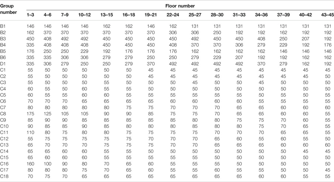
TABLE 4. Member sizes for the structural system. D1 indicates diagonals while W24 sections are identified through their weight per unit length using imperial units. Box sections are identified in terms of their mid-line width in cm.

Envelop System

Each glass panel was mounted 0.5 m from the upper floor and 1.5 m from the lower floor. The cladding system was considered not to provide lateral stiffness. The equivalent net pressure demand was defined as follows:

$p_{eq}\left(t;{\xi }_{xyz}\right)={\left(\frac{1}{t_{eq}}{\int }_0^t{\left[p_n\left(t;{\xi }_{xyz}\right)\right]}^s\right)}^{\frac{1}{s}}(33)$

with t_eq = 60 s and s = 16. The damage state $D{S}_{P_{60}}$ was considered terminal. In calibrating the coupled damage model of Section 5.2.1, the occurrence of $D{S}_{D{r}_1}$ or $D{S}_{D{r}_2}$ was considered to result in an reduction in capacity to resist p_eq of 10 and 80%, respectively. To account for uncertainty, the reductions were taken as the means of truncated normal distributions of support [0,1] and coefficient of variation of 0.1. All damage states were considered to require the replacement of the glazing unit. In calibrating the model of Section 6, a single consequence function was therefore required. The median values of the consequence function were as follows: Q_min = 20, Q_max = 100, Q_max = 2,955 (USD), and Q_min = 1,576 (USD). Uncertainty was modeled through assigning a log-normal distribution of dispersion of 0.1185 to the consequence function.

Wind-Driven Rain Simulation

The normalized specific catch ratios necessary for calibrating the interpolation-based scheme of Section 4.2 were estimated in OpenFOAM 4.1. Three computational domains were considered for wind angles of α_H = 0°, α_H = 45°, and α_H = 90°. Each domain extended, at full scale, 900 m upwind/laterally and 2,700 m downwind of the building. Each domain had a total of 139,500 rectangular elements in a structured mesh. Seventeen rain phases were considered with raindrop diameters ranging from 0.3 to 2.4 mm with a 0.3 mm increment and from 2.4 to 6 mm with an increment of 0.4 mm. Through symmetry, the simulation results were extended to wind directions of 135°, 180°, 225°, 270°, and 315°. Solutions were estimated for the wind speeds defining the boundaries of the nine conditional failure events used in deriving the hazard curve of Section 8.2.