Parameter Calibration of a Social Force Model for the Crowd-Induced Vibrations of Footbridges

A reliable prediction of the human-induced vibrations of footbridges relies on an accurate representation of the pedestrian excitation for different loading scenario. Particularly, the modeling of crowd-induced dynamic loading is a critical issue for the serviceability assessment of footbridges. At the design stage, the modeling of crowd loading is often derived from single pedestrian models, neglecting the effect of the structural vibrations as well as the interactions among pedestrians. A detailed description of the crowd behavior can be achieved employing a social force model that describes the different influences affecting individual pedestrian motion. These models are widely adopted to describe the crowd behavior especially in the field of evacuation of public buildings, public safety and transport station management while applications in the serviceability assessment of footbridges are less common. To simulate unidirectional pedestrian flows on footbridges, this paper proposes a parameter calibration of the Helbing’s social force model performed adopting the response surface methodology. Parameters of the social force model are calibrated so as to represent the fundamental relation between mean walking speed and density of the pedestrian crowd. The crowd-induced vibrations are then simulated by modeling each pedestrian in the crowd as a vertical load that crosses the footbridge with time varying trajectory and velocity estimated from the calibrated social force model. Finally, results are compared to those obtained from a multiplication factor approach proposed in literature. This considers the crowd as a uniform distribution of pedestrians with constant speed and given synchronization level and the footbridge response is evaluated as the response to a single pedestrian scaled by a proper enhancement factor.

1 Introduction

The serviceability assessment under pedestrian-induced vibrations is a key aspect in the design of modern footbridges, which are usually slender and light structures. This can make them particularly vulnerable to human-induced vibrations. The great interest of the scientific community in the serviceability assessment of modern footbridges has been mainly motivated by swaying problems experienced by several long-span footbridges such as the Millenium Bridge in London (Dallard et al., 2001) and the Solferino footbridge in Paris (Danbon and Grillaud, 2005). However, this is not a new phenomenon and also earlier researches can be found in the literature (Matsumoto et al., 1978; Fujino et al., 1993). In the last 20 years, much efforts were devoted to the characterization of the load induced by a single pedestrian walking or running and the subsequent extrapolation of these findings to the case of a moving crowd (Racic et al., 2009; Caprani et al., 2012; Pan et al., 2017; Younis et al., 2017; Bassoli et al., 2018a; Wang et al., 2019). Some of these studies have contributed to the publication of several guidelines and standards for the design of slender footbridges under pedestrian action, such as Butz et al. (2008). However, codes of practice still present some shortages, especially when dealing with pedestrian crowds. In those cases, in fact, the simulated dynamic response often differs from the experimental evidence (Živanović et al., 2010; da Silva et al., 2013). This is mainly due to the simplified crowd models adopted, based on an enhancement factor related to the pedestrian number that multiplies the single person load.

Recently, new important aspects of the pedestrian behavior have been introduced and taken into account to improve the modeling of pedestrian crowds, which are the crowd behavior, the human-structure interaction and the inter- and intra-subject variability of the walking force (Venuti et al., 2016; Jiménez-Alonso and Sáez, 2017; Bassoli et al., 2018b; Moreu et al., 2020). The latter is usually simulated adopting a probabilistic approach, namely modeling the walking parameters as random variables (Živanović et al., 2007; Van Nimmen et al., 2014, 2020). Several models able to address the three above mentioned key aspects have been proposed, among which da Silva et al. (2013); Venuti et al. (2016); Jiménez-Alonso and Sáez (2017). They share a common pattern based on the coupling of two sub-models: a pedestrian-structure interaction model and a crowd model. The most common approach, but not the only one, to model the pedestrian-structure interaction is to represent each pedestrian as a single degree of freedom (SDOF) system crossing the structure in addition to a external force attached to its base. The external force represents the walking force caused on a rigid surface while the SDOF system contributes to modify the dynamic properties of the crowd-structure coupled system (Venuti et al., 2016). As far as the crowd behavior is concerned, two modeling approaches exist: macroscopic and microscopic models. The firsts are based on the modeling of the crowd behavior as a continuous flow of a fluid. The second models allow for a more detailed description of the crowd thanks to the evaluation of the time varying position and velocity of each pedestrian. Macroscopic models consider the behavior of the crowd as a whole and assume the continuity of flow, assumption that may not be satisfied for low and medium pedestrian densities (Carroll et al., 2012). Moreover, the variability in the walking parameters among the crowd cannot be accounted for. The above mentioned limitations can be overcome adopting the microscopic modeling, in which the behavior of each pedestrian is governed by the different motivations and influences that he/she experiences according to the equations of particle dynamics (Jiménez-Alonso et al., 2016). This approach was initially proposed by Helbing and Molnar (1995), who described the various stimuli experienced by each pedestrian in the crowd as social forces. This allows to consider that i) the pedestrian crowd may not be uniformly distributed, ii) each pedestrian can contribute differently to the modal excitation depending on his own pacing frequency and iii) pedestrians may react by stopping or slowing down depending on the perceived level of footbridge vibrations (Carroll et al., 2012).

Social force models (SFM) have been widely adopted to simulate the behavior of pedestrian crowds in the fields of transport station management, safety assurance of large pedestrian flow events and building evacuation (Chen et al., 2018). Their large diffusion depends on the good capability of describing movement processes using simple mathematical formulations. Starting from the original version proposed by Helbing and Molnar (1995), different developments have been proposed to adapt the model to the application field. A comprehensive review summarizing the existing social force models for pedestrian traffic is presented in Chen et al. (2018). Furthermore, some applications of social force models for the serviceability assessment of footbridges under pedestrian flows can be also found in literature, both with reference to lateral (Carroll et al., 2012) and vertical (Jiménez-Alonso et al., 2016; Venuti et al., 2016) loads. The crowd model adopted by Carroll et al. (2012) is adapted from the one proposed by Langston et al. (2006) and based on the findings of Helbing et al. (2000). In particular, Langston et al. (2006) studied a multi-circle pedestrian model to simulate a single enclosure entry scenario. However, the calibration of the parameter describing pedestrian rotational movements remains a challenging task. Moreover, the parameters adopted in Helbing et al. (2000) are chosen to simulate the mechanisms of panic and jamming by uncoordinated motion in crowds. Similarly, social force model parameters adopted in Jiménez-Alonso et al. (2016) are based on Carroll et al. (2012) and Helbing and Molnar (1995). In the latter case, simulations are performed to describe the self-organization of collective phenomena of pedestrian behavior considering two pedestrian groups trying to pass a narrow door and walking in opposite directions. Finally, Venuti et al. (2016) adopt a crowd model originally proposed by Cristiani et al. (2011) who described the interaction mechanisms by velocity terms.

This paper proposes a parameter calibration of the Helbing’s social force model (Helbing et al., 2005) for the vibration serviceability of footbridges. For a realistic simulation of the pedestrian traffic, model parameters are adjusted so that the simulated pedestrian flow fits the fundamental speed-density relation proposed by Weidmann (1993). The optimization process is carried out adopting the response surface methodology (RSM), based on the approximation of the objective function using simple analytical functions. The RSM is widely adopted in model optimization problems thanks to an adequate accuracy of results combined with computational efficiency (Vincenzi and Savoia, 2015; Myers et al., 2016). Once the social force model is properly calibrated, simulations are performed for different pedestrian flows allowing for the evaluation of the time-varying position and velocity of each pedestrian in the crowd. These are adopted as input data for detailed simulations of the pedestrian-induced loads on a step-by-step basis. Finally, simulation results are compared to those obtained from a multiplication factor approach proposed by Caprani et al. (2012). Based on the assumption that the crowd is composed of uniformly distributed pedestrians with constant speed and given synchronization level, they calculate enhancement factors to evaluate the footbridge response to crowd loads scaling the single pedestrian load.

The paper is organized as follows. The basics of the social force model are presented in section 2. Section 3 describes how the simulated speed-density relation is obtained starting from the results of the social force model. The optimal model parameters are evaluated in section 4 and the calibrated social force model is adopted in section 5 to simulate crowd-induced vibrations. Results are compared to those obtained adopting a multiplication factor approach in section 6. Finally, conclusions are drawn in section 7.

2 The Social Force Model

The social force model describes the behavior of individual pedestrians by a superposition of social forces that reflect motivations and environmental influences. The motivation to move toward a specific destination with a certain desired velocity is represented by a driving term, while repulsive forces describe the tendency to keep a certain distance from other pedestrians, borders, obstacles, and dangers. Finally, attractive forces express the tendency of a group or family members to stay together or to move towards window displays, sights or unusual events. The basics of the social force model are shown in the following, while the reader is referred to Helbing and Molnar (1995); Helbing et al. (2000, 2005) for a detailed description.

The time-varying velocity of a generic pedestrian α, ${\mathit{v}}_{\alpha }\left(t\right)$, is governed by the equation of motion as follows:

$\frac{\text{d}{\mathit{x}}_{\alpha }\left(t\right)}{\text{d}t}={\mathit{v}}_{\alpha }\left(t\right)(1)$

where ${\mathit{x}}_{\alpha }\left(t\right)=\left\{X_{\alpha }\left(t\right),Y_{\alpha }\left(t\right)\right\}$ is a vector collecting his/her time-varying positions in X and Y direction, which are, respectively, parallel and orthogonal to the footbridge centerline. Similarly, ${\mathit{v}}_{\alpha }\left(t\right)=\left\{v_{X,\alpha }\left(t\right),v_{X,\alpha }\left(t\right)\right\}$. Positions and velocities are in m and m/s, respectively. Acceleration or deceleration of pedestrian α is expressed:

$\frac{\text{d}{\mathit{v}}_{\alpha }\left(t\right)}{\text{d}t}={\mathit{f}}_{\alpha }\left(t\right)+{\mathit{\xi }}_{\alpha }\left(t\right)(2)$

In Eq. 2, ${\mathit{f}}_{\alpha }\left(t\right)$ is the overall social force representing the sum of different systematic influences on the behavior of pedestrian α and ${\mathit{\xi }}_{\alpha }\left(t\right)$ are the random behavioral fluctuations caused by accidental or intentional variations from the optimal behavior. Note that, according to Helbing et al. (2005), Eq. 2 is defined considering a unitary pedestrian mass, implying that the social force has the same dimensions as an acceleration (m/s²). The acceleration force ${\mathit{f}}_{\alpha }\left(t\right)$ of pedestrian α is the sum of a driving force ${\mathit{f}}_{\alpha }^0\left({\mathit{v}}_{\alpha }\right)$, repulsive interactions with other pedestrians β ${\mathit{f}}_{\alpha \beta }\left({\mathit{x}}_{\alpha },{\mathit{x}}_{\beta }\right)$, repulsive effects due to boundaries ${\mathit{f}}_{\alpha i}\left({\mathit{x}}_{\alpha }\right)$, and attraction effects ${\mathit{f}}_{\alpha z}\left({\mathit{x}}_{\alpha },{\mathit{x}}_z\right)$:

${\mathit{f}}_{\alpha }\left(t\right)={\mathit{f}}_{\alpha }^0\left({\mathit{v}}_{\alpha }\right)+{\displaystyle \sum }_{\beta \ne \alpha }^{N_P}{\mathit{f}}_{\alpha \beta }\left({\mathit{x}}_{\alpha },{\mathit{x}}_{\beta }\right)+{\displaystyle \sum }_i{\mathit{f}}_{\alpha i}\left({\mathit{x}}_{\alpha }\right)+{\displaystyle \sum }_z{\mathit{f}}_{\alpha z}\left({\mathit{x}}_{\alpha },{\mathit{x}}_z\right)(3)$

where N_P is the total number of pedestrians in the simulation. The social force, pedestrian positions and velocities are all function of time t. However, this dependency may be omitted in the following equations for the sake of simplicity.

The driving term represents i) the intention of each pedestrian to walk with a desired speed $v_{\alpha }^0$ into the direction ${\mathit{e}}_{\alpha }^0$ of its destination and ii) the fact that deviations of the actual velocity ${\mathit{v}}_{\alpha }\left(t\right)$ from the desired velocity ${\mathit{v}}_{\alpha }^0=v_{\alpha }^0{\mathit{e}}_{\alpha }^0$ are corrected within the relaxation time ${\tau }_{\alpha }$:

${\mathit{f}}_{\alpha }^0\left({\mathit{v}}_{\alpha }\right)=\frac{1}{{\tau }_{\alpha }}\left(v_{\alpha }^0{\mathit{e}}_{\alpha }\left(t\right)-{\mathit{v}}_{\alpha }\left(t\right)\right)(4)$

where ${\mathit{e}}_{\alpha }\left(t\right)$ is the desired direction of motion. The desired direction of motion is given by:

${\mathit{e}}_{\alpha }\left(t\right)=\frac{{\mathit{x}}_{\alpha }^k-{\mathit{x}}_{\alpha }\left(t\right)}{\Vert {\mathit{x}}_{\alpha }^k-{\mathit{x}}_{\alpha }\left(t\right)\Vert }(5)$

where ${\mathit{x}}_{\alpha }\left(t\right)$ is the actual position of pedestrian α at time t while ${\mathit{x}}_{\alpha }^k$ is the next edge of an imaginary polygon with edges ${\mathit{x}}_{\alpha }^1,\dots ,{\mathit{x}}_{\alpha }^n={\mathit{x}}_{\alpha }^0$ representing the shortest way to the desired destination ${\mathit{x}}_{\alpha }^0$.

The interaction repulsive forces describe that the pedestrian α tends to keep a situation-dependent distance from the other pedestrians β:

${\mathit{f}}_{\alpha \beta }\left(t\right)=A_{\alpha ,1}\text{exp}\left(\frac{r_{\alpha \beta }-d_{\alpha \beta }}{B_{\alpha ,1}}\right){\mathit{n}}_{\alpha \beta }\left({\lambda }_{\alpha }+\left(1-{\lambda }_{\alpha }\right)\frac{1+\text{cos}{\phi }_{\alpha \beta }}{2}\right)+A_{\alpha ,2}\text{exp}\left(\frac{r_{\alpha \beta }-d_{\alpha \beta }}{B_{\alpha ,2}}\right){\mathit{n}}_{\alpha \beta }(6)$

The first term of the right-hand side of Eq. 6 describes the territorial effect, namely the tendency to respect the private sphere of each pedestrian, and helps avoiding collisions if there are sudden velocity changes. The second term express physical interactions at high pedestrian densities and pushy crowds, when frictional effects are ignored. Note that other definitions of the repulsive force can be found in literature, such as the velocity dependent interaction force described in Johansson et al. (2008) and Helbing and Johansson (2009). However, Johansson et al. (2008) pointed out that the prediction of pedestrian motion does not significantly improve by including additional speed-dependent parameters, in light of an increasing computational time and complexity. The parameters A_α and B_α identify the repulsive interaction strength and range, respectively, and partially depend on cultural influences. Although the dependence on α would enable defining those parameters for each individual, it is usually assumed $A_{\alpha }=A$ and $B_{\alpha }=B$. This allows avoiding a too large number of parameters that complicates model calibration. $d_{\alpha \beta }$ is the distance between the centers of mass of pedestrians α and β while $r_{\alpha \beta }=r_{\alpha }+r_{\beta }$ is the sum of their radii. The assumption of an homogeneous population leads to $r_{\alpha }=r_{\beta }$. The parameter ${\mathit{n}}_{\alpha \beta }\left(t\right)$ is the normalized vector pointing from pedestrian β to α. Finally, the parameter ${\lambda }_{\alpha }$ allows to account for the anisotropic nature of pedestrian interactions. This means that a pedestrian is typically more influenced by pedestrians in front that those behind. ${\phi }_{\alpha \beta }\left(t\right)$ is the angle between the desired direction of motion ${\mathit{e}}_{\alpha }\left(t\right)$ and the direction $-{\mathit{n}}_{\alpha \beta }\left(t\right)$ of the pedestrian exerting the repulsive force. It follows that $\text{cos}{\phi }_{\alpha \beta }\left(t\right)=-{\mathit{n}}_{\alpha \beta }\left(t\right){\mathit{e}}_{\alpha }\left(t\right)$. Figure 1 shows how the parameter ${\lambda }_{\alpha }$ influences the shape of the area around the pedestrian where the territorial effects act. The anisotropic pedestrian behavior is taken into account considering ${\lambda }_{\alpha }$ values less than one. It is observed from Figure 1 that when ${\lambda }_{\alpha }$ decreases the action area of the territorial effects is more concentrated in front of the pedestrian.

FIGURE 1

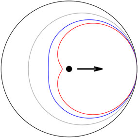
FIGURE 1. Action area of the territorial effects for a pedestrian (black dot) moving to the right considering different ${\lambda }_{\alpha }$ values: ${\lambda }_{\alpha }=1$ (black), ${\lambda }_{\alpha }=0.6$ (gray), ${\lambda }_{\alpha }=0.3$ (blue), ${\lambda }_{\alpha }=0.1$ (red).

Furthermore, pedestrians tend to keep a certain distance from borders, such as guardrails or walls. The repulsive effect of borders is similar to the repulsion among pedestrians except for the anisotropic behavior. It is described by a force ${\mathit{f}}_{\alpha i}\left(t\right)$ monotonically decreasing with the distance $d_{\alpha i}$ between the boundary i and the pedestrian α:

${\mathit{f}}_{\alpha i}\left(t\right)=A_{\alpha i}\text{exp}\left(\frac{r_{\alpha }-d_{\alpha i}}{B_{\alpha i}}\right){\mathit{n}}_{\alpha i}(7)$

Similarly to the repulsive interaction among pedestrians, $A_{\alpha i}$ and $B_{\alpha i}$ are the repulsive strength and range and ${\mathit{n}}_{\alpha i}$ is the vector pointing from the boundary i to the pedestrian α.

Pedestrian behavior can also be affected by the so-called attractive effects, which represent the tendency of pedestrian groups, such as family members or tourist groups, to walk together. These attractive forces can be modeled accordingly to the repulsive forces among pedestrians of Eq. 6 with longer interaction range and negative interaction strength.

The social force model of Eqs. (1–7) is described by $4\times N_P$ first order ordinary differential equations. The first 2 × N_P differential equations define the X and Y velocity components for pedestrians 1 to N_P (Eq. 2), while the second 2 × N_P differential equations characterize the corresponding positions (Eq. 1). The system of differential equations can be solved numerically through a MATLAB routine starting from the initial velocity and position of each pedestrian.

3 Evaluation of the Simulated SPEED-DENSITY Relation

This section shows how the speed-density relation can be evaluated from the results of the social force model. First, input parameters and assumptions made for the simulations of the pedestrian flow are listed in section 3.1, while an example of the simulated speed-density relation is presented in section 3.2.

3.1 Problem Formulation

The desired velocity of each pedestrian $v_{\alpha }^0$ is considered as the typical pedestrian velocity in unrestricted traffic conditions, which can be described by a normally distributed random variable with a mean of 1.34 m/s and a standard deviation of 0.26 m/s (Buchmüller and Weidmann, 2006). To prevent unrealistic values, the desired speed is limited to the range [0.5–2.2] m/s.

As regards the repulsive force among pedestrians, the first term of the right-hand side of Eq. 6 is considered, which represents the tendency to respect the private pedestrian sphere and accounts for the anisotropic pedestrian behavior. It is assumed that the repulsive force between two pedestrians acts when $d_{\alpha \beta }\le 2r_{\alpha \beta }$. This allows avoiding the unrealistic behavior for which two pedestrians change their trajectory ever since they are far apart.

The model parameters to be calibrated are $r_{\alpha }$ and ${\lambda }_{\alpha }$, which characterize the pedestrian radius and the anisotropic human behavior, respectively, as well as the interaction strength and range $A_{\alpha ,1}$ and $B_{\alpha ,1}$ of Eq. 6. On the contrary, values of relaxation time ${\tau }_{\alpha }$ and interaction strength and range with borders $A_{\alpha i}$ and $B_{\alpha i}$ are assumed accordingly to the literature. Fixed values of these parameters are listed in Table 1. This choice is motivated as follows. The pedestrian behavior depends on the relative amplitude of the forces acting on him/her (driving force, repulsive interaction with other pedestrians and with borders). This means that the amplitudes of the different social forces are not independent but the same results could be obtained from different combinations of parameters. Based on this consideration, parameters of the interaction repulsive forces among pedestrians are assumed as calibration parameters while the amplitude of the driving force is fixed. Moreover, also the parameters of the repulsive effect of borders are assumed according to the typical values proposed in literature because they result sufficiently high to prevent the pedestrians to get off the footbridge.

TABLE 1

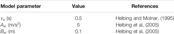
TABLE 1. Fixed values of the social force model parameters.

Because the destination of a pedestrian crossing the footbridge is typically the opposite end and not a specific point, the desired destination is re-evaluated at each iteration. By doing this, in the event of interaction with other pedestrians or with the borders, the pedestrian is able to re-evaluate its desired destination as the point on the footbridge edge closest to its current position (Parry, 2007).

Finally, according to applications of the social force model found in literature, attractive effects ${\mathit{f}}_{\alpha z}\left({\mathit{r}}_{\alpha },{\mathit{r}}_z\right)$ and random fluctuations ${\mathit{\xi }}_{\alpha }\left(t\right)$ are neglected (Helbing and Molnar, 1995; Johansson et al., 2008; Wei et al., 2017).

3.2 Simulated Speed-Density Relation

Simulations are performed considering a footbridge 10 m long and 3 m wide. The footbridge is completed by an access route 60 m long and a 300 m long way out (Figure 2). Access road and way out are necessary for the modeling of a roughly stationary pedestrian flow on the footbridge. Initial pedestrian positions are randomly distributed in the access route. Considering that the dimension of each pedestrian is 2r_α, the uniform random distribution of initial positions is defined on the condition that pedestrians shall not overlap. An example of the random initial positions of a pedestrian group is presented in Figure 2. Finally, the way out needs to be long enough so as not to stop the pedestrian flow in the central part.

FIGURE 2

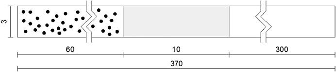
FIGURE 2. Geometry of the footbridge (gray) and of the access route and way out (white). Black dots: example of random initial positions of pedestrians. Dimensions are in meters.

To define the simulated speed-density relation, simulations are repeated for different-sized pedestrian groups. In particular, groups of 25 to 500 pedestrians are considered. As results depend on the random initial position and velocity of each pedestrians, for each group dimension the simulation is repeated 10 times to increase the number of results (namely N_A = 10). The total analysis duration ranges from 125 to 195 s depending on the group dimension. The analysis duration is chosen so as to allow approximately all pedestrians to cross the footbridge.

The social force model allows for the evaluation of the positions and velocities (both in X and Y direction) of each pedestrian during the whole analysis. As the parameters of interest are limited to the footbridge (highlighted in gray in Figure 2), results related to positions in X direction between 60 and 70 m are extracted and analyzed in the rest of the paper. Figure 3A shows an example of the number of pedestrians present on the footbridge at each time instant for the case of 350 pedestrians. It can be observed that the pedestrian number gradually increases at the beginning of the analysis. Once the majority of pedestrians arrived on the footbridge, the pedestrian number remains roughly constant as long as they start leaving the footbridge. Density and velocity of people walking are evaluated according to two different criteria:

FIGURE 3

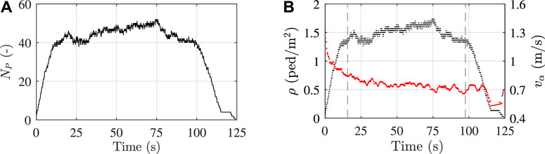
FIGURE 3. (A) Number of pedestrians on the footbridge and (B) instantaneous crowd density (black dots) and velocity (red dots) for the case of 350 pedestrians.

• Criterion 1: crowd density and mean pedestrian velocity are evaluated at each time instant. An example of the instantaneous velocity and density obtained for the case of 350 pedestrians is shown in Figure 3B. The analysis can be ideally divided in three time windows: 0 − T₁, T₁ − T₂, and T₂ − T_end. T₁ and T₂ represent the first and the last time instant when the 80% of N_P,max pedestrians is on the footbridge, being N_P,max the maximum number of pedestrians simultaneously present on the footbridge. As regards the example of Figure 3B, T₁ = 15.7 s, T₂ = 97.5 s and T_end = 125 s. In the first time window, the mean pedestrian velocity decreases as the pedestrian density increases, while in the central part of the analysis they remain roughly stationary. Finally, from T₂ to T_end the pedestrian density decreases since pedestrians start leaving the footbridge. In this case, a decreasing pedestrian density does not correspond to an increasing mean velocity as pedestrians are not free to move but they are slowed down by pedestrians that have already left the footbridge. To avoid meaningless results, instantaneous densities and velocities are evaluated up to T₂. Instantaneous values can be represented in a speed-density diagram, as shown in Figure 4A, where the relation between increasing density and decreasing mean velocity can be clearly observed.

FIGURE 4

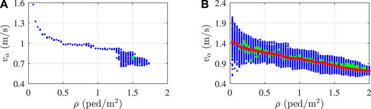
FIGURE 4. (A) Example of the crowd density and velocity from criterion 1 (blue dots) and criterion 2 (green dot) for the case of 350 pedestrians (B) example of the crowd density and velocity from criterion 1 (blue dots) and criterion 2 (green dots) and simulated speed-density relation (red dots) for group dimensions from 25 to 500 pedestrians.

• Criterion 2: mean pedestrian density and velocity are evaluated over the central time window of the analysis (T₁ − T₂), namely when the pedestrian flow is roughly stationary. With the reference to the previous example, this results in the green dot of Figure 4A.

Figure 4B presents an example of the speed-density diagram obtained considering results from criterion 1 and criterion 2 for different analyses, namely 11 pedestrian group sizes and 10 analyses for each case. Finally, the simulated speed-density relation represented by red dots is obtained from criterion 1 by evaluating the mean crowd velocity in correspondence of each pedestrian density.

4 Model Parameter Calibration

The social force model described above is calibrated so that the simulated pedestrian flow fits the fundamental speed-density relation presented by Venuti and Bruno (2007) in the form:

$v_m\left(\rho \right)=v_u\left\{1-\text{exp}\left[-\gamma {\rho }_{jam}\left(\frac{1}{\rho }-\frac{1}{{\rho }_{jam}}\right)\right]\right\}(8)$

where $v_m\left(\text{m}/\text{s}\right)$ is the mean crowd velocity, $v_u\left(\text{m}/\text{s}\right)$ is the free-flow speed, γ (−) is a parameter depending on the travel purpose and ${\rho }_{jam}\left(\text{ped}/{\text{m}}^2\right)$ is the jam density, i. e., the pedestrian density associated with completely stopped traffic flow. Eq. 8 is a generic form of the velocity-density relation originally proposed by Weidmann (1993), the so called Kladek formula. By assuming γ = 0.354, ${\rho }_{jam}=5.4\text{ ped}/{\text{m}}^2$ and $v_u=1.34\text{ m}/\text{s}$, Eq. 8 matches the original one (Ferrarotti and Tubino, 2015). The trend of the speed-density relation obtained assuming the above mentioned parameters is represented by the black curve of Figure 6. The curve is limited to the pedestrian density range [0–2] ped/m² being it the range of interest for vibration assessment purposes. The fundamental speed-density relation represents a macroscopic model of pedestrian movements as it treats the crowd as a continuous and homogeneous fluid.

The model is calibrated through the response surface methodology, a widely adopted mathematical and statistical method for modeling and analyzing processes in which the response of interest is affected by various variables. The aim of the RSM is to find the values of input variables that produce the best value of the response (Myers et al., 2016). This study means to find the values of the model parameters to be calibrated, i.e., ${\lambda }_{\alpha }$, $r_{\alpha }$, $B_{\alpha ,1}$ and $A_{\alpha ,1}$, such as to minimize the discrepancy between the simulated and theoretical speed-density relation. This is achieved through the minimization of an objective function H defined as the mean squared error between the simulated and theoretical speed-density relation. In particular, in this study values of the first three optimization parameters are evaluated through the RSM assuming A_α,1 = 2 m/s², evaluated through preliminary analyses. Successively, the value of $A_{\alpha ,1}$ is adjusted close to the optimal solution. The RMS has been successfully adopted in several applications for solving model optimization problems thanks to its limited computational effort (Pula and Bauer, 2007; Hariri-Ardebili et al., 2018). The RSM is briefly described in section 4.1 and is adopted in section 4.2 to find the optimal values of the model parameters.

4.1 Response Surface Methodology

The basic idea of the RSM is to approximate the objective function using simple and explicit interpolation functions. Originally proposed by Box and Winson (1951) to optimize chemical processes, the application of RSM has been subsequently extended to other fields such as engineering problems involving complex and time consuming analyses in order to reduce the computational effort (Vincenzi and Savoia, 2015).

According to the RSM, the objective function H can be approximated by an analytical estimation function $\widehat{H}$:

$\widehat{H}=g\left(\mathbf{p}\right)(9)$

with p the D-dimensional vector collecting the model parameters to be calibrated and $g\left(\mathbf{p}\right)$ the response function. In the classic RSM, the response function is usually obtained by combining first or second-order polynomials that fit the objective function calculated in a set of sampling points. The typical choice of second-order approximations is motivated by an adequate accuracy of results combined with the computational efficiency. Higher order polynomials are rarely used because of the increasing number of coefficients that need to be identified. The main drawback in the use of a quadratic response surface (RS) lies in the fact that it predicts the presence of a single minimum also when the actual objective function presents more local minima (Vincenzi and Savoia, 2015). To get over this limitation, the RSM has to be applied in a region close to the optimal solution. Hence, Eq. 9 can be re-written as a second-order polynomial function:

$\widehat{H}=\frac{1}{2}{\mathbf{p}}^{\text{T}}\mathbf{Q}\mathbf{p}+\mathbf{L}\mathbf{p}+{\beta }_0(10)$

where Q is a D × D matrix gathering the quadratic terms, L is a D-dimension vector collecting the linear coefficient and β₀ a constant.

Khuri and Cornell (1996) proposed the procedure described in the following to analytically correlate values of identification parameters and $\widehat{H}$ using a limited number of selected numerical simulations. For the sake of simplicity and without loss of generality, the procedure is described considering three calibration parameters, i.e., $\mathbf{p}=\left\{p_1,p_2,p_3\right\}$. Under this assumption, Eq. 10 becomes:

$\widehat{H}\left(x_1,x_2\right)={\beta }_0+{\beta }_1{p}_1+{\beta }_2{p}_2+{\beta }_3{p}_3+{\beta }_4{p}_1^2+{\beta }_5{p}_2^2+{\beta }_6{p}_3^2+{\beta }_7{p}_1{p}_2+{\beta }_8{p}_1{p}_3+{\beta }_9{p}_2{p}_3(11)$

where β_i are the unknown coefficients of the RS. Considering NS observations, namely NS evaluation of $\widehat{H}$ starting from NS different vectors p, Eq. 11 can be written in matrix form as:

$\widehat{H}=\mathbf{Z}\mathit{\beta }(12)$

where ${\mathit{\beta }}^{\text{T}}=\left\{{\beta }_0,{\beta }_1,\dots {\beta }_9\right\}$ is a vector collecting the unknown coefficients of the response surface, Z is a matrix containing the constant, linear, quadratic and cross terms polynomial terms and $\widehat{H}$ is a vector that collects NS values of the objective functions. For a better definition of the response surface, the number of observations NS has to be grater than the number of parameters collected in β (Vincenzi and Savoia, 2015). Vector β is determined through the least squares estimation method as follows:

$\mathit{\beta }={\left({\mathbf{Z}}^{\text{T}}\mathbf{Z}\right)}^{-1}{\mathbf{Z}}^{\text{T}}\widehat{H}(13)$

In Eq. 13, all observations have the same weight. To increase the accuracy of the RS close to the optimal solution, Kaymaz and McMahon (2005) and Myers et al. (2016) proposed the weighted regression method where weights of sampling points $\mathbf{p}$ close to the optimal solution are increased:

$\mathit{\beta }={\left({\mathbf{Z}}^{\text{T}}\mathbf{W}\mathbf{Z}\right)}^{-1}{\mathbf{Z}}^{\text{T}}\mathbf{W}\widehat{H}(14)$

where w is a NS × NS diagonal matrix of weight coefficients. The weight coefficients w_i can be evaluated as (Vincenzi and Savoia, 2015):

$w_i=\text{exp}\left(-\frac{g\left({\mathbf{p}}_i\right)-H_{\text{best}}}{H_{\text{best}}}\right)(15)$

where

$H_{\text{best}}=\text{min}\left(g\left({\mathbf{p}}_i\right)\right)(16)$

Once the parameters β of the response surface are evaluated, the optimal parameter vector p^* minimizing $\widehat{H}$ is computed as:

${\mathbf{p}}^{\text{*}}=-{\mathbf{Q}}^{-1}\mathbf{L}(17)$

Finally, the estimation of the optimal solution is further improved by iteratively re-calibrating the response surface close to p^*. A detailed flowchart of the updating process is presented in Figure 5.

FIGURE 5

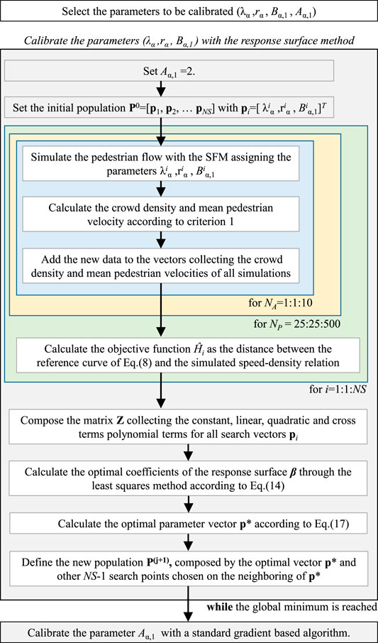
FIGURE 5. Flowchart of the updating process. $N_A$ is the number of analyses performed for each case.

4.2 Results and Discussion

Results of the social force model calibration are presented in Table 2 and Figure 6. Table 2 lists the ranges of variation and the optimal values of the updating parameters, while Figure 6 shows the speed-density relation obtained from the calibrated social force model together with the theoretical curve. In this case, the simulated speed-density relation is calculated considering six pedestrian group dimensions (from 250 to 500 pedestrians) and 10 analyses for each case. A pretty good agreement between the theoretical and simulated curve can be observed, even though slightly higher discrepancies are found for very low densities (ρ< 0.3 ped/m²).

TABLE 2

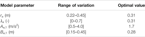
TABLE 2. Ranges of variation and optimal values of the updating parameters.

FIGURE 6

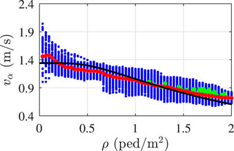
FIGURE 6. Crowd density and velocity from criterion 1 (blue dots) and criterion 2 (green dots) and simulated speed-density relation (red dots) obtained from the calibrated model. Black curve: theoretical speed-density relation.

As an example,Figures 7A,B show, respectively, the effect of the model parameter $A_{\alpha ,1}$ and $B_{\alpha ,1}$ on the simulated speed-density relation. In particular, Figure 7A is obtained by considering the optimal values of the model parameters except for $A_{\alpha ,1}$ which is assumed equal to 0.5 m/s². As the strength of the interaction among pedestrians is reduced, they are free to move more independently. This results in the fact that the mean crowd velocity barely decreases with increasing pedestrian density but rather it remains approximately equal to the free-flow velocity. An opposite effect is caused by the increasing of the interaction range $B_{\alpha ,1}$, which is assumed equal to 1 m in Figure 7B (while values of the other parameters are those listed in Table 2). In this case, pedestrian interactions are such as to significantly reduce the mean crowd velocities when the pedestrian density increases and make it impossible to reach pedestrian densities higher than about 1.5 ped/m².

FIGURE 7

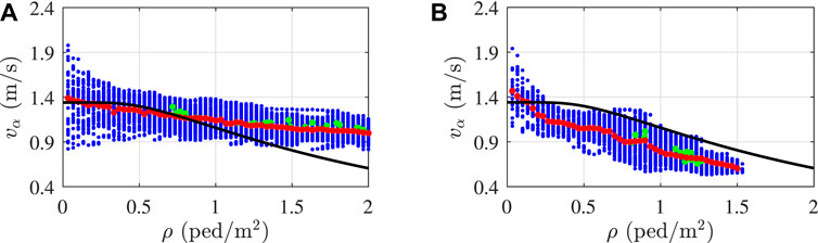
FIGURE 7. Crowd density and velocity from criterion 1 (blue dots) and criterion 2 (green dots) and simulated speed-density relation (red dots) obtained considering (A)$A_{\alpha ,1}$ = 0.5 m/s² and (B)$B_{\alpha ,1}$ = 1 m. Black curve: theoretical speed-density relation.

To assess the reliability of results, the optimal simulated speed-density relation is also compared to experimental measurements of pedestrian flows reported in literature. In particular, results presented by Oeding (1963), Older (1968), Mōri and Tsukaguchi (1987), Fruin (1987), Weidmann (1993) and Seyfried et al. (2005) are considered. Note that the results presented by Weidmann (1993) represent a fitting of the experiments and they are the basis from which the analytical model of Eq. 8 was obtained. Calibration results are in line with the experiments although the high variability of these latter.

Finally, the effect of the footbridge geometry on the simulated speed-density relation is evaluated. Results obtained considering a footbridge width of 2.5, 4.5 and 7.0 m are compared to those obtained from the reference width of 3.0 m in Figure 8B. It is firstly observed that an increase in the footbridge width does not affect the results while a narrower footbridge implies a slightly lower curve. This is because in the second case the repulsive effects of borders further limit the pedestrian density on the footbridge. On the contrary, increasing the footbridge geometry implies that the same mean pedestrian densities and velocities can be reached. Accordingly, the footbridge length does not affect the simulated speed-density relation, unless very short and unusual footbridges are considered. However, for each geometry variation, the pedestrian group size needed to reach a certain pedestrian density has to be evaluated as well as an adequate length of the access route and way out.

FIGURE 8

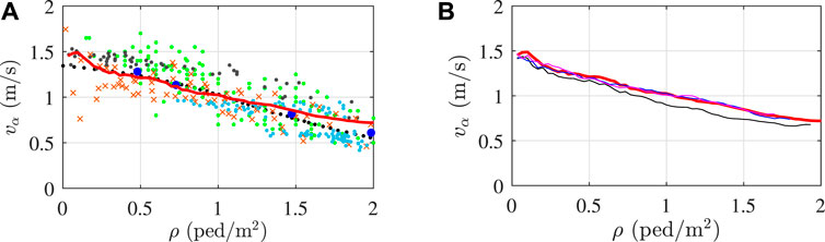
FIGURE 8. (A) Comparison between the simulated speed-density relation (red curve) and experimental measurements of pedestrian flows. Black dots: Weidmann (1993), green dots: Oeding (1963), grey dots: Mōri and Tsukaguchi (1987), orange crosses: Older (1968), light blue dots: Seyfried et al. (2005), blue circles: Fruin (1987)(B) Simulated speed-density relations obtained considering different footbridge width: 3.0 m (red curve), 2.5 m (black curve), 4.5 m (blue curve) and 7.0 m (magenta curve).

5 Pedestrian Flow Simulations

This section presents the footbridge vibrations induced by pedestrian flows simulated through the calibrated social force model.

5.1 Footbridge Parameters

The footbridge considered in the simulations is a simply supported beam 10 m long and 3 m wide having a linear dynamic behavior. It is characterized by a modal mass of 25 × 10³ kg, a damping ratio of 0.5% and a natural frequency varying from 0.5 to 3.0 Hz. Only the contribution of the fundamental mode, namely the first bending mode having a half-sine mode shape, is taken into account.

5.2 Crowd Loading

The crowd loading is given by the superposition of the walking forces induced by each pedestrian in the crowd. The single pedestrian walking force is obtained as a series of successive footfall forces, each one described as a Fourier series according to the model proposed by Li et al. (2010). In particular the jth footstep force of a generic pedestrian α is expressed:

$P_{\alpha }^j\left(t\right)=G_{\alpha }{\displaystyle \sum }_{n=1}^{5}DL{F}_{n,\alpha }^j\text{sin}\left(\frac{\pi n}{T_{c,\alpha }^j}t\right),0\le t\le T_{c,\alpha }^j(18)$

where $DL{F}_{n,\alpha }^j$ (-) are the Fourier coefficients normalized to the weight of the pedestrian $G_{\alpha }$ (N) and $T_{c,\alpha }^j$ (s) is the step duration, namely the duration of the contact between the foot and the ground. The step duration $T_{c,\alpha }^j$ is related to the step period $T_{s,\alpha }^j$ by $T_{c,\alpha }^j=T_{s,\alpha }^j+\text{Δ}t$, where $\text{Δ}t=0.24T_{c,\alpha }^j$. The single step force is defined accounting for the contribution of the first five harmonics. Values of the Fourier coefficients for the five harmonics are defined for step frequencies in the range [1.60–2.40] Hz and can be found in Li et al. (2010). Application points and walking parameters of each single step force are evaluated starting from the results of the social force model as shown in the following.

The next scheme outlines how the walking force of a generic pedestrian α in the crowd is evaluated:

•The pedestrian weight $G_{\alpha }$ is randomly extracted from a log-normal distribution with a mean of 73.85 kg and a standard deviation of 15.68 kg (Portier et al., 2007).

•The trajectory of pedestrian α is evaluated from the results of the SFM, as the one shown in Figure 9 (black line).

•Application points of the single foot forces are identified on the pedestrian trajectory placing them at a distance of $l_{s,\alpha }^j$. The length of each step $l_{s,\alpha }^j$ is evaluated from the pedestrian velocity v and the step frequency $f_s$ through the relation $v=l_{s,\alpha }^j{f}_s\left(v\right)$. Pedestrian velocity and step length for each step are estimated through an iterative procedure such that the velocity adopted to calculate the step length matches the velocity estimated from the SFM in the successive foot standing point (reached taking a step of that length). Velocity and step frequency are related through the following Eq. 19. With reference to the previous example, this results in the red dots of Figure 9.

•As the contribution of the first bending mode is taken into account, the 2-D problem can be reduced to a 1-D problem by projecting the foot standing points on the footbridge centerline (green dots in Figure 9). Note that this simplification would not be appropriate if a torsional mode contributed to the structural response.

•Instants of application of the single foot forces are evaluated as the instants when pedestrian α occupies the positions identified by red dots in Figure 9. Note that the initial time when the pedestrian starts to walk on the footbridge depends on its initial position as well as the path followed in the 60 m preceding the footbridge (Figure 2). Moreover, this method allows accounting for the fact that a pedestrian may stop walking and then restart. In this case, in fact, a larger time gap between two successive steps would be observed.

•The velocity in correspondence of each step is obtained by combining the instantaneous velocities in X and Y directions. Figure 10A presents the time varying position (in X direction) and velocity of the same pedestrian of Figure 9. Blue and red dots identify velocities and positions of the considered footsteps along with the corresponding instants of application.

•For each footstep j, the velocity magnitude is converted into a pacing frequency through the following relation proposed by Bruno and Venuti (2008) based on the experimental data presented in Bertram and Ruina (2001):

$f_{s,\alpha }^j=0.35{\left(v_{\alpha }^j\right)}^3-1.59{\left(v_{\alpha }^j\right)}^2+2.93v_{\alpha }^j(19)$

•where $f_{s,\alpha }^j$ is expressed in Hz and $v_{\alpha }^j$ in m/s. The applicability limits for this empirical relation can be assumed either as $v_{\alpha }^j=[0.2-2.5]\text{ m}/\text{s}$ or $v_{\alpha }^j=[0.23-2.2]\text{ m}/\text{s}$, in accordance with Bruno and Venuti (2008) or Bertram and Ruina (2001), respectively.

•The period $T_{s,\alpha }^j$ is evaluated from $f_{s,\alpha }^j$ as $T_{s,\alpha }^j=1/f_{s,\alpha }^j$. The step duration $T_{c,\alpha }^j$ is, in turn, obtained as $T_{s,\alpha }^j+\text{Δ}t$.

•Starting from the pedestrian weight $G_{\alpha }$ and the step duration $T_{c,\alpha }^j$, the single foot force $P_{\alpha }^j\left(t\right)$ is evaluated through Eq. 18.

•Finally, the single pedestrian walking force is obtained by adding the contribution of all footstep forces, each one applied in the position and at the time instant previously evaluated.

FIGURE 9

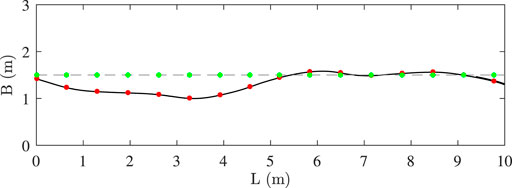
FIGURE 9. Example of pedestrian trajectory (black line), foot positions on the trajectory (red dots) and projection of the foot positions on the bridge centerline (green dots).

FIGURE 10

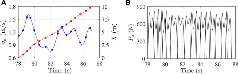
FIGURE 10. Example of (A) pedestrian velocities (blue line and dots) and positions in X direction (red line and dots) vs. time and (B) consecutive footfall forces.

Figure 10B shows the temporal sequence of footstep forces for the pedestrian α, which have to be added to obtain the single pedestrian walking force. This procedure is repeated for each pedestrian in the crowd and, finally, the crowd loading is obtained by the superposition of the individual pedestrian forces.

5.3 Footbridge Response Simulation

The footbridge response is evaluated by numerically integrating the equation of motion in the modal space considering the footbridge as a single degree of freedom system and time increments of 0.001 s (see, for instance, Bassoli et al. (2018a)). To calculate the modal force, the crowd loading of Section 5.2 is weighted by the amplitude of the mode shape in correspondence of the footfall positions. The variable representative of the response is chosen as the mid-span acceleration. The vibration response is assessed using a 1-s root-mean-square (RMS) moving average value from the acceleration time history.

Finally, the effects of the crowd-bridge interaction in terms of added mass are evaluated. In particular, the mean number of pedestrians simultaneously present on the footbridge during the time interval T₁ − T₂ (section 3.2) is added to the footbridge mass and the corresponding reduction in the footbridge natural frequency is estimated.

5.4 Results and Discussion

In the following, results obtained for pedestrian groups of 100 and 350 pedestrians are presented. Table 3 lists the values of the mean density and velocity obtained from criterion 2 (see section 3.2) for each of the 10 analyses performed, together with the mean walking frequency estimated from Eq. 19. Simulations with 100 pedestrians lead to mean pedestrian densities ranging from 0.51 to 0.84 ped/m² and corresponding velocities from 1.20 to 1.02 m/s², while 350 pedestrians involve densities in the range [1.61–1.90] ped/m² and velocities from 0.85 to 0.78 m/s². Velocities from criterion 2 give an indication of the pedestrian velocity. However, in the crowd load simulations, the velocity of each pedestrian is evaluated on a step-by-step basis as detailed in section 5.2. Note that group dimensions of 100 and 350 pedestrians are chosen as representative of correlated and very dense traffic, respectively. In the first case pedestrian movements are not completely free but partially constrained by the presence of other pedestrians, while in the second case they are highly constrained by other pedestrians. Moreover, it has to be stressed that the Fourier coefficients of Eq. 18 are defined for step frequencies in the range [1.60–2.40] Hz. Nevertheless, numerical simulations are performed considering also frequencies out of this range, as a consequence of the velocities involved.

TABLE 3

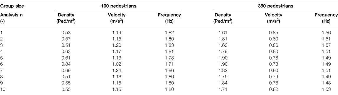
TABLE 3. Mean densities and velocities from criterion 2 and corresponding frequencies.

The maximum RMS accelerations obtained for pedestrian groups of 100 and 350 pedestrians and for footbridge natural frequencies in the range [0.5–3.0] Hz are shown in Figure 11. In particular, for each group size and for each natural frequency the footbridge response is evaluated 10 times starting from the results of the 10 SFM simulations. These results are indicated with black dots in Figure 11, while mean values are highlighted in red. As expected, accelerations caused by 100 pedestrians are lower than those due to 350 pedestrians. The main amplifications of the structural response are obtained for frequencies between 1.5 and 2 Hz for the case of 100 pedestrians, while they are observed also for lower structural frequencies in the second case. This is an effect of the lower pedestrian velocities (and consequently step frequencies) characterizing higher pedestrian densities. Moreover, it is observed that, in both cases, amplifications of the structural response are obtained for a wide range of footbridge frequencies because each pedestrian in the crowd contributes differently to the modal excitation depending on his own pacing frequency, which changes step-by-step.

FIGURE 11

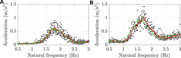
FIGURE 11. Maximum RMS accelerations caused by (A) 100 and (B) 350 pedestrians for different footbridge natural frequencies: results for each of the 10 analyses (black dots) and mean values (red line). Green dotted line: mean accelerations obtained accounting for the added pedestrian mass.

Finally, the effects of the pedestrian mass are evaluated. The mean number of pedestrians simultaneously present on the footbridge during the time interval $T_1-T_2$ is 20 and 54 for the case of 100 and 350 pedestrians, respectively. As also shown in Figure 3A, the number of pedestrians on the footbridge is significantly lower than the pedestrian group size considered in the analyses. Indeed, this latter is necessary to obtain a roughly stationary pedestrian flow with a certain density. The presence of 20 and 54 pedestrians causes a reduction of the footbridge natural frequency of 1.42% and 3.64%, respectively. Mean accelerations obtained accounting for the effects of the pedestrian mass are represented by the dashed green light in Figure 11. Considering, for instance, a footbridge natural frequency of 2 Hz, the added pedestrian mass causes a reduction of the acceleration by 2.9% and 12.1% for the case of 100 and 350 pedestrians, respectively.

6 Comparison

Results of section 5 are compared with those obtained from the multiplication factor approach proposed by Caprani et al. (2012). In particular, they evaluate a set of enhancement factors for predicting the response due to a crowd based on the predicted accelerations of a single pedestrian. Enhancement factors are evaluated for crowd densities ranging from 0.44 ped/m² to 2.11 ped/m² (namely 0.44, 0.55, 0.75, 1.5 and 2.11 ped/m²) and synchronization proportions of 0, $\sqrt{N}$, 0.135, 0.2, 0.5, 0.75N and N, being N the pedestrian number. This latter represents the proportion of pedestrians considered to be synchronized with each other, namely walking in phase at the same frequency. In addition, they consider footbridge natural frequencies of 1.94, 2.0 and 2.1 Hz. The crowd loading enhancement factor m is defined as the ratio of the characteristic response due to the crowd to the characteristic response due to a single pedestrian. Consistent with the aim of this work, enhancement factors obtained without taking into account crowd-structure interaction are considered.

In this study, the single pedestrian load is based on the single step load model of Li et al. (2010) (Eq. 18). In contrast to the crowd loading of section 5.2, in this case it is assumed that the pedestrian produces the same footfall force at each step leading to a periodic walking force. In line with Caprani et al. (2012), the pedestrian weight G and step length $l_s$ are assumed equal to, respectively, 73.85 kg and 0.66 m (Barela and Duarte, 2008), while the pedestrian velocity is evaluated from the results of the social force model according to the criterion 2 (Table 3). This means to consider that the single pedestrian is moving with a velocity corresponding to the mean crowd velocity. For the purpose of comparison, results for natural frequencies of 1.94, 2.0 and 2.1 Hz are presented. Hence, for each pedestrian group and footbridge natural frequency, 10 values of the single pedestrian acceleration are calculated considering the pedestrian velocities of Table 3. Finally, the multiplication factors m are evaluated as the ratio of the crowd-induced acceleration to the corresponding single pedestrian acceleration.

Multiplication factors are plotted in Figure 12 together with the values of m proposed by Caprani et al. (2012). The multiplication factor obtained from each simulation is associated to the corresponding mean crowd density listed in Table 3. Results from 350 pedestrians, representing crowd densities typical of constrained traffic, are mainly consistent with those proposed by Caprani et al. (2012) for synchronization levels from 0.5N to N. On the contrary, results from 100 pedestrians, describing densities typical of correlated but not constrained traffic, are in quite good agreement with those of Caprani et al. (2012) for synchronization proportion lower than 0.2N. This findings are in line with the fact that pedestrians tend to synchronize more and more with increasing crowd density.

FIGURE 12

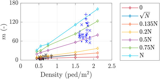
FIGURE 12. Multiplication factors m obtained from 100 pedestrians (black markers) and 350 pedestrians (blue markers) for footbridge natural frequencies of 1.94 Hz (.), 2.0 Hz (+) and 2.1 Hz (×). Colored lines: multiplication factors of Caprani et al. (2012) for different synchronization proportions.

7 Conclusions

This paper proposes a parameter calibration of the Helbing’s social force model (Helbing et al., 2005) performed adopting the response surface methodology. Model parameters are calibrated so as to describe the fundamental relation between mean walking speed and density of pedestrian crowds. The calibrated social force model enables a detailed simulation of unidirectional pedestrian flows on footbridges suitable for vibration assessment purposes. The updated model is adopted in this paper to simulate pedestrian flows and results are compared with the multiplication factor approach proposed by Caprani et al. (2012).

The speed-density relation obtained from the calibrated social force model shows a pretty good match with the theoretical curve, with larger discrepancies observed for ρ < 0.3 ped/m². However, the simulated curve obtained considering $A_{\alpha ,1}=0.5$ ped/m² fits very well the theoretical curve up to pedestrian densities of 0.5 ped/m². This value can be adopted to simulate unconstrained pedestrian traffic alternately to the optimal value. Finally, calibration results demonstrate the importance of a proper model parameter calibration. Indeed, it is highlighted that changes in the model parameters imply an inaccurate description of the crowd behavior, which does not represent the theoretical one assumed as reference.

The social force model allows for the evaluation of the instantaneous position and velocity of each pedestrian in the crowd, assumed as the input of a step-by-step simulation of the pedestrian loads. Simulations presented in the paper highlight the advantages of a discrete crowd model, that is the direct possibility of modeling the variability of the crowd loading and the suitability for low and medium traffic densities and discontinuous pedestrian distribution. being the traffic continuity not required.

The main drawback of the presented crowd model is that analyses can be time-consuming, especially for high pedestrian densities. Moreover, the random nature of the crowd loading requires a statistical characterization of the response, incrementing the computing time.

It is worth noting that the proposed calibrated parameters are adequate to simulate pedestrian flows on footbridge with different dimensions than those adopted in this study, with exception of width lower than 3.0 m. In these case, in fact, the simulated speed-density relation is slightly lower. However, for each geometry variation, the pedestrian group size needed to reach a certain pedestrian density has to be evaluated as well as an adequate length of the access route and way out.

The comparison with the multiplication factors proposed by Caprani et al. (2012) shows a good agreement with the simulation results, even though they are scattered. In particular, the coherence of multiplication factors obtained for high pedestrians densities with those of Caprani et al. (2012) for high levels of synchronization, and vice versa for low pedestrian densities, demonstrates the ability of the model to describe the crowd behavior without the need to define in advance the synchronization level.

Data Availability Statement

The original contributions presented in the study are included in the article, further inquiries can be directed to the corresponding author.

Author Contributions

Conceptualization, EB and LV; Data collection, EB and LV; Analysis and interpretation of results, EB and LV; Supervision, LV; Writing, review and editing, EB and LV.

Conflict of Interest

The authors declare that the research was conducted in the absence of any commercial or financial relationships that could be construed as a potential conflict of interest.

References

Barela, A. M. F., and Duarte, M. (2008). Biomechanical Characteristics of Elderly Individuals Walking on Land and in Water. J. Electromyogr. Kinesiol. 18, 446–454. doi:10.1016/j.jelekin.2006.10.008

PubMed Abstract | CrossRef Full Text | Google Scholar

Bassoli, E., Gambarelli, P., and Vincenzi, L. (2018a). Human-induced Vibrations of a Curved Cable-Stayed Footbridge. J. Constructional Steel Res. 146, 84–96. doi:10.1016/j.jcsr.2018.02.001

CrossRef Full Text | Google Scholar

Bassoli, E., Van Nimmen, K., Vincenzi, L., and Van den Broeck, P. (2018b). A Spectral Load Model for Pedestrian Excitation Including Vertical Human-Structure Interaction. Eng. Structures 156, 537–547. doi:10.1016/j.engstruct.2017.11.050

CrossRef Full Text | Google Scholar

Bertram, J. E. A., and Ruina, A. (2001). Multiple Walking Speed-Frequency Relations Are Predicted by Constrained Optimization. J. Theor. Biol. 209, 445–453. doi:10.1006/jtbi.2001.2279

PubMed Abstract | CrossRef Full Text | Google Scholar

Box, G. E. P., and Wilson, K. B. (1951). On the Experimental Attainment of Optimum Conditions. J. R. Stat. Soc. Ser. B (Methodological). 13, 1–38. doi:10.1111/j.2517-6161.1951.tb00067.x

CrossRef Full Text | Google Scholar

Bruno, L., and Venuti, F. (2008). The Pedestrian Speed-Density Relation: Modelling and Application. in Proceedings Of the 3rd International Footbridge Conference, Porto, Portugal

Google Scholar

Buchmüller, S., and Weidmann, U. (2006). Parameters of Pedestrians, Pedestrian Traffic and Walking Facilities. Tech. rep., ETH Zürich, IVT. 132, 1–58. doi:10.3929/ethz-b-000047950

CrossRef Full Text | Google Scholar

Butz, C., Feldmann, M., Heinemeyer, C., and Sedlacek, G. (2008). Advanced Load Models for Synchronous Pedestrian Excitation and Optimised Design Guidelines for Steel Footbridges. Tech. rep., Res. Fund Coal Steel

Google Scholar

Caprani, C. C., Keogh, J., Archbold, P., and Fanning, P. (2012). Enhancement Factors for the Vertical Response of Footbridges Subjected to Stochastic Crowd Loading. Comput. Structures. 102-103–103, 87–96. doi:10.1016/j.compstruc.2012.03.006

PubMed Abstract | CrossRef Full Text | Google Scholar

Carroll, S. P., Owen, J. S., and Hussein, M. F. M. (2012). Modelling Crowd-Bridge Dynamic Interaction with a Discretely Defined Crowd. J. Sound Vibration 331, 2685–2709. doi:10.1016/j.jsv.2012.01.025

CrossRef Full Text | Google Scholar

Chen, X., Treiber, M., Kanagaraj, V., and Li, H. (2018). Social Force Models for Pedestrian Traffic - State of the Art. Transport Rev. 38, 625–653. doi:10.1080/01441647.2017.1396265

CrossRef Full Text | Google Scholar

Cristiani, E., Piccoli, B., and Tosin, A. (2011). Multiscale Modeling of Granular Flows with Application to Crowd Dynamics. Multiscale Model. Simul. 9, 155–182. doi:10.1137/100797515

CrossRef Full Text | Google Scholar

da Silva, F. T., Brito, H. M. B. F., and Pimentel, R. L. (2013). Modeling of Crowd Load in Vertical Direction Using Biodynamic Model for Pedestrians Crossing Footbridges. Can. J. Civ. Eng. 40, 1196–1204. doi:10.1139/cjce-2011-0587

CrossRef Full Text | Google Scholar

Dallard, P., Fitzpatrick, T., Bourva, S. L., Low, A., Smith, R. R., and Willford, M. (2001). The London Millennium Footbridge. The Struct. Engineer. 79, 17–33.

Google Scholar

Danbon, F., and Grillaud, G. (2005). Dynamic Behaviour of a Steel Footbridge. Characterization and Modelling of the Dynamic Loading Induced by a Moving Crowd on the Solferino Footbridge in Paris. in Proceedings Of the 2nd International Footbridge Conference (Venice, Italy)

Google Scholar

Ferrarotti, A., and Tubino, F. (2015). Equivalent Spectral Model for Pedestrian-Induced Forces on Footbridges: a Generalized Formulation. in Proceedings Of the 5th ECCOMAS Thematic Conference On Computational Methods In Structural Dynamics And Earthquake Engineering (Crete Island, Greece). doi:10.7712/120115.3551.800

CrossRef Full Text | Google Scholar

Fruin, J. J. (1987). Pedestrian Planning and Design. Mobile: Elevator World, Inc

Fujino, Y., Pacheco, B. M., Nakamura, S.-I., and Warnitchai, P. (1993). Synchronization of Human Walking Observed during Lateral Vibration of a Congested Pedestrian Bridge. Earthquake Engng. Struct. Dyn. 22, 741–758. doi:10.1002/eqe.4290220902

CrossRef Full Text | Google Scholar

Hariri-Ardebili, M. A., Seyed-Kolbadi, S. M., and Noori, M. (2018). Response Surface Method for Material Uncertainty Quantification of Infrastructures. Shock and Vibration. 2018, 1, 14. doi:10.1155/2018/1784203

CrossRef Full Text | Google Scholar

Helbing, D., Buzna, L., Johansson, A., and Werner, T. (2005). Self-organized Pedestrian Crowd Dynamics: Experiments, Simulations, and Design Solutions. Transportation Sci. 39, 1–24. doi:10.1287/trsc.1040.0108

CrossRef Full Text | Google Scholar

Helbing, D., Farkas, I., and Vicsek, T. (2000). Simulating Dynamical Features of Escape Panic. Nature. 407, 487–490. doi:10.1038/35035023

PubMed Abstract | CrossRef Full Text | Google Scholar

Helbing, D., and Johansson, A. (2009). Pedestrian, Crowd and Evacuation Dynamics. New York, NY: Springer New York, 6476–6495. doi:10.1007/978-0-387-30440-3_382

CrossRef Full Text

Helbing, D., and Molnár, P. (1995). Social Force Model for Pedestrian Dynamics. Phys. Rev. E. 51, 4282–4286. doi:10.1103/PhysRevE.51.4282

CrossRef Full Text | Google Scholar

Jiménez-Alonso, J. F., Sáez, A., Caetano, E., and Magalhães, F. (2016). Vertical Crowd-Structure Interaction Model to Analyze the Change of the Modal Properties of a Footbridge. J. Bridge Eng. 21. doi:10.1061/(ASCE)BE.1943-5592.0000828

CrossRef Full Text | Google Scholar

Jiménez-Alonso, J. F., and Sáez, A. (2017). Recent Advances in the Serviceability Assessment of Footbridges under Pedestrian-Induced Vibrations. Bridge Eng. Chapter 5. doi:10.5772/intechopen.71888

CrossRef Full Text | Google Scholar

Johansson, A., Helbing, D., and Shukla, P. K. (2007). Specification of the Social Force Pedestrian Model by Evolutionary Adjustment to Video Tracking Data. Advs. Complex Syst. 10, 271–288. doi:10.1142/S0219525907001355

CrossRef Full Text | Google Scholar

Kaymaz, I., and McMahon, C. A. (2005). A Response Surface Method Based on Weighted Regression for Structural Reliability Analysis. Probabilistic Eng. Mech. 20, 11–17. doi:10.1016/j.probengmech.2004.05.005

CrossRef Full Text | Google Scholar

Khuri, A. I., and Cornell, J. A. (1996). Response Surfaces: Designs and Analyses, 2nd Edition (Boca Raton: CRC Press). doi:10.1201/9780203740774

CrossRef Full Text

Langston, P. A., Masling, R., and Asmar, B. N. (2006). Crowd Dynamics Discrete Element Multi-Circle Model. Saf. Sci. 44, 395–417. doi:10.1016/j.ssci.2005.11.007

CrossRef Full Text | Google Scholar

Li, Q., Fan, J., Nie, J., Li, Q., and Chen, Y. (2010). Crowd-induced Random Vibration of Footbridge and Vibration Control Using Multiple Tuned Mass Dampers. J. Sound Vibration. 329, 4068–4092. doi:10.1016/j.jsv.2010.04.013

CrossRef Full Text | Google Scholar

Mōri, M., and Tsukaguchi, H. (1987). A New Method for Evaluation of Level of Service in Pedestrian Facilities. Transportation Res. A: Gen. 21, 223–234. doi:10.1016/0191-2607(87)90016-1

CrossRef Full Text | Google Scholar

Matsumoto, Y., Nishioka, T., Shiojiri, H., and Matsuzaki, K. (1978). Dynamic Design of Footbridges. IABSE Proc. 1–15. doi:10.5169/seals-33221

Google Scholar

Moreu, F., Maharjan, D., Zhu, C., and Wyckoff, E. (2020). Monitoring Human Induced Floor Vibrations for Quantifying Dance Moves: A Study of Human-Structure Interaction. Front. Built Environ. 6, 36. doi:10.3389/fbuil.2020.00036

CrossRef Full Text | Google Scholar

Myers, R. H., Montgomery, D. C., and Anderson-Cook, C. M. (2016). Response Surface Methodology: Process and Product Optimization Using Designed Experiments. 4th Edition. Wiley Series in Probability and Statistics (Wiley)

Oeding, D. (1963). Verkehrsbelastung und Dimensionierung von Gehwegen und anderen Anlagen des Fußgängerverkehrs (Strassenbau und Strassenterkehrstechnik). Bonn: German

Older, S. (1968). Movement of Pedestrians on Footways in Shopping Streets. Traffic Eng. Control. 10, 160–163.

Google Scholar

Pan, S., Xu, S., Mirshekari, M., Zhang, P., and Noh, H. Y. (2017). Collaboratively Adaptive Vibration Sensing System for High-Fidelity Monitoring of Structural Responses Induced by Pedestrians. Front. Built Environ. 3, 28. doi:10.3389/fbuil.2017.00028

CrossRef Full Text | Google Scholar

Parry, G. W. (2007). The Dynamics Of Crowds. Master’s thesis. Dordrecht: Department of Mathematical Sciences - University of Bath. doi:10.1007/1-4020-5312-6

CrossRef Full Text | Google Scholar

Portier, K., Keith Tolson, J., and Roberts, S. M. (2007). Body Weight Distributions for Risk Assessment. Risk Anal. 27 (1), 11–26. doi:10.1111/j.1539-6924.2006.00856.x

PubMed Abstract | CrossRef Full Text | Google Scholar

Pula, W., and Bauer, J. (2007). Probabilistic Methods in Geotechnical Engineering (Vienna: Springer), Vol. 491 of CISM Courses And Lectures, Chap. Application of the Response Surface Method. doi:10.1007/978-3-211-73366-0_6

CrossRef Full Text

Racic, V., Pavic, A., and Brownjohn, J. M. W. (2009). Experimental Identification and Analytical Modelling of Human Walking Forces: Literature Review. J. Sound Vibration. 326, 1–49. doi:10.1016/j.jsv.2009.04.020

CrossRef Full Text | Google Scholar

Seyfried, A., Steffen, B., Klingsch, W., and Boltes, M. (2005). The Fundamental Dyagram of Pedestrian Movements Revisited. J. Stat. Mech. 10, P10002. doi:10.1088/1742-5468/2005/10/p10002

Google Scholar

Van Nimmen, K., Lombaert, G., Jonkers, I., De Roeck, G., and Van den Broeck, P. (2014). Characterisation of Walking Loads by 3D Inertial Motion Tracking. J. Sound Vibration. 333, 5212–5226. doi:10.1016/j.jsv.2014.05.022

CrossRef Full Text | Google Scholar

Van Nimmen, K., Van den Broeck, P., Lombaert, G., and Tubino, F. (2020). Pedestrian-induced Vibrations of Footbridges: An Extended Spectral Approach. J. Bridge Eng. 25, 04020058. doi:10.1061/(ASCE)BE.1943-5592.0001582

CrossRef Full Text | Google Scholar

Venuti, F., and Bruno, L. (2007). An Interpretative Model of the Pedestrian Fundamental Relation. Comptes Rendus Mécanique. 335, 194–200. doi:10.1016/j.crme.2007.03.008

CrossRef Full Text | Google Scholar

Venuti, F., Racic, V., and Corbetta, A. (2016). Modelling Framework for Dynamic Interaction between Multiple Pedestrians and Vertical Vibrations of Footbridges. J. Sound Vibration 379, 245–263. doi:10.1016/j.jsv.2016.05.047

CrossRef Full Text | Google Scholar

Vincenzi, L., and Savoia, M. (2015). Coupling Response Surface and Differential Evolution for Parameter Identification Problems. Computer-Aided Civil Infrastructure Eng. 30, 376–393. doi:10.1111/mice.12124

CrossRef Full Text | Google Scholar

Wang, Y., Brownjohn, J., Dai, K., and Patel, M. (2019). An Estimation of Pedestrian Action on Footbridges Using Computer Vision Approaches. Front. Built Environ. 5, 133. doi:10.3389/fbuil.2019.00133

CrossRef Full Text | Google Scholar

Wei, X., Broeck, P. V. d., Roeck, G. D., and Nimmen, K. V. (2017). A Simplified Method to Account for the Effect of Human-Human Interaction on the Pedestrian-Induced Vibrations of Footbridges. Proced. Eng. 199, 2907–2912. doi:10.1016/j.proeng.2017.09.331International Conference on Structural Dynamics, EURODYN 2017

CrossRef Full Text | Google Scholar

Weidmann, U. (1993). Transporttechnik der Fussgänger. Report no. 90. ETH Zürich: IVT

Younis, A., Avci, O., Hussein, M., Davis, B., and Reynolds, P. (2017). Dynamic Forces Induced by a Single Pedestrian: A Literature Review. Appl. Mech. Rev. 69. doi:10.1115/1.4036327

CrossRef Full Text | Google Scholar

Živanović, S., Pavić, A., and Ingólfsson, E. (2010). Modeling Spatially Unrestricted Pedestrian Traffic on Footbridges. J. Struct. Eng. ASCE 136, 1296–1308. doi:10.1061/(ASCE)ST.1943-541X.0000226

Google Scholar

Živanović, S., Pavić, A., and Reynolds, P. (2007). Probability-based Prediction of Multi-Mode Vibration Response to Walking Excitation. Eng. Structures 29, 942–954. doi:10.1016/j.engstruct.2006.07.004

Google Scholar