Influence of Socioeconomic Factors on Transit Demand During the COVID-19 Pandemic: A Case Study of Bogotá’s BRT System

The COVID-19 pandemic restricted most economic and social activities, impacting travel demand for all transportation modes and especially for transit. We hypothesize that the shifts in travel demand varied by socioeconomic status, and we assess the differential impact of COVID-19 in the Bus Rapid Transit (BRT) patronage across various socioeconomic groups in Bogotá. We built a database of frequent transit users with data collected by smartcards in Bogota’s BRT system between January and October 2020. For each user in the database, we labeled their home and work stations. Transactions at other stations are classified as “other.” The stratum (a government socioeconomic classification of residential units in Colombia) of a BRT station’s service area was assigned using an estimated probability vector for each user belonging to a specific stratum; this data is validated with aggregate strata distributions in the 2019 household travel survey. Our study found that the reduction in transactions for lower-strata users is significantly less than that of the middle and high strata. The magnitude of this difference varies over time but stabilizes after the end of the lockdown. The growth rate of “other” transactions per thousand people is greater than the growth for home and work locations, especially for the lowest strata. Other studies have shown that the radius of gyration (Rg) (a measure of how far individuals travel away from home) has decreased about 50% after the lockdowns. Our study shows that when measuring Rg only for users who continued using BRT, the Rg slightly decreased for lower and medium strata but increased for high strata. The contribution of this study is a method to classify BRT transactions of frequent users by strata, as well as a description of trends in BRT use by strata to expand our understanding of the COVID-19 lockdowns impacts in the Global South context. These results are a starting point to inform policy and decision-makers to guide the recovery efforts to improve transit accessibility and level of service for captive users such as low-stratum users.

1 Introduction

One of the major effects of the COVID-19 outbreak and the lockdowns is the drastic reduction of transit demand. In China, mode share for metro dropped from 26 to 14% (Institute for Transportation and Development Policy, 2020). In Europe and North America, transit ridership declined by as much as 90% during the first weeks of the lockdown measures (TransitApp, 2020a). Likewise, the Inter-America Development Bank shows a ridership reduction of 60 to 90% in major cities across Latin America (Inter-American Development Bank, 2020).

Since the beginning of the outbreak, many studies have shown a differential impact of the lockdowns on minorities and vulnerable groups, such as women (Alon et al., 2020), low-income groups (Sumner et al., 2020), and small businesses (Fairlie, 2020). However, in transportation, most of the analyses have focused on understanding general behavioral change in travel patterns and mode shares. For instance, Huang et al. (2020) used passive data from a routing app to analyze travel times by mode, type of visited locations, and preference of origins and destinations. An ongoing study in Switzerland, using GPS data of 250 participants, shows that train and tram use remains constant at a 60% reduction compared to the baseline, but daily bike distance increased 100% on average (Molloy et al., 2020). Similarly, Teixeira and Lopes (2020) found that the average trip time for the bike-sharing system at New York increased from 13 to 19 min at dock stations near metro stations. In terms of public transit, Orro et al. (2020) found a more significant demand reduction in transit stops near schools, universities, and supermarkets.

There is a growing literature that explores the impact on transportation demand by socioeconomic group. For example, Astroza et al. (2020), using a convenience sample survey of 4,395 individuals in Chile, found that 77% of workers from low-income households do not telecommute. A survey of more than 25,000 transit users in North America showed that pandemic-era riders are primarily low-income essential workers with no private vehicle access (TransitApp, 2020b). Using smartcard data, researchers have found a correlation between socioeconomics and transit use reduction. These studies infer socioeconomic variables, such as income, by different fare values (Brough et al., 2020) or by matching census data and with home boarding stations (Almlöf et al., 2020; Wilbur et al., 2020). Dueñas et al. (2020) used smartcard data in Bogota to explore the relationship between transit and strata, informality, and poverty. The study found that lower strata, higher informality, and higher poverty correlated with more transit reduction use. However, this study linked a transaction to the characteristics of the area rather than the individual. Therefore, a transaction of a low-strata user in a high-income area may have counted as a high-strata transaction.

While the literature suggests that travel shifts during COVID-19 have varied by socioeconomic group, little is known about what changes will persist and how the evolution will vary by group. Wang et al. (2020) showed that behavioral inertia caused by the pandemic might result in public transit demand of only 73% compared to pre-pandemic levels in New York, but they do not investigate how this might vary among socioeconomic groups. The governments’ role is to provide a safe and efficient transit system (World Health Organization, 2020). As people have continued to use transit to access essential services and jobs during the pandemic, transit agencies should consider adjusting their services to better accommodate the populations that most depend on them (The International Association of Public Transport, 2020). Therefore, it is critical to assess and understand the evolution of transit demand disaggregated by socioeconomic group. An assessment of this kind is necessary to plan transit operations with a vertical equity objective in mind (i.e., allocating services to where they are most needed) rather than horizontal equity (i.e., allocating services proportionally to everyone) (Camporeale et al., 2017). While surveys provide an opportunity to explore the differences in transit demand with rich socioeconomic variables, they are costly and time-consuming. Actions and decisions need to be taken nearly in real-time.

This study assesses and describes the change and evolution of the transit demand by different socioeconomic group during the COVID-19 pandemic in Bogota. We leveraged smartcard data from Bogota’s Bus Rapid Transit (BRT) system to assess the differential impact of the COVID-19 pandemic restrictions by socioeconomic groups. Although the data does not contain any socioeconomic variables, we use inference methods (Pappalardo et al., 2019; Pérez-Messina et al., 2020) to obtain a probability distribution for one socioeconomic variable in the context of Bogota. Our research objectives are 1) to infer socioeconomic characteristics of frequent BRT users based on smartcard data, and 2) to use this information to expand our understanding of the COVID-19 lockdowns impacts and trends on transit demand by strata. While changes in the supply may cause changes in the demand, and changes in demand may also cause changes in supply, this two-way causality is not possible to address with the available data. Therefore, this is not an objective of our study.

The remainder of this paper is organized as follows. Section 2 provides the background information on Bogota, its transit system, and the COVID-19 timeline. Section 3 summarizes the methodology we used to build a database of frequent users. Section 4 introduces the three main findings of this research related to transit use change by strata. In Section 5, we conduct an extensive discussion of the results. Section 6 presents the study limitations and future research. Finally, in Section 7, we state the conclusion of this study.

2 Background

Bogota is the largest city in Colombia; according to the 2018 census, it has a population of 7.2 million. The 2019 Household Travel Survey (HTS) estimated that 30% of the trips, or about 4.5 million trips, are made daily in the public transit system. Bogota’s transit system has two main components, the BRT and the Integrated Public Transit System (SITP, for its acronym in Spanish). The BRT system has 152 stations, three cable car stations, and 2.5 million transactions a day (Transmilenio S.A., 2020a). Passengers use a contactless card to validate at entry points only; there is no need to validate the exit point as the system uses a flat fare.

Bogota has a stratum classification, which is an official socioeconomic variable assigned to every residential unit in Colombia. Strata ranges from one to six depending on physical characteristics of the building (such as construction materials, built squared meters, type and quality of finishes), the environment (such as dominant topography, dominant constructive typification, dominant densities, and public utilities accessibility and coverage), and the urban context (land use, and characteristics and access to the road network) (DANE, 2015). According to Law 142 of 1994, the purpose of this classification is to provide a differential charge for public utilities, apportion subsidies, and charge extra contributions. Note that the stratum is attached to a physical dwelling but not to a specific individual. While strata do not consider household income, Cantillo-Garcia et al. (2019) concluded that it is justifiable to understand it as a proxy for income: low-strata correlates with lower-income and high-strata with higher-income. Many studies in transportation have used strata as a predictor variable in travel behavior (Munoz-Raskin, 2010; Bocarejo S. and Oviedo H., 2012; Delmelle and Casas, 2012).

Like many cities and countries, Bogota and Colombia declared a lockdown in March 2020 aiming to reduce the spread of the COVID-19 virus, which halted most of the region’s economic activities. Unlike the United States, Europe, and China, the lockdown measure in Bogota and Colombia was preventive. The early lockdown allowed time to prepare the health system for a future wave of COVID-19 patients (MinSalud, 2020). Bogota’s mayor decreed a drill lockdown on March 20, and then the national government declared a mandatory lockdown on March 24 that lasted until September 1. In April, the government required transit systems to operate at 35% capacity in an effort to stop the spread of the virus. The peak-and-plate measure, a policy that restricts private vehicle use on certain days depending on the last digit of the vehicle’s plate, was lifted to avoid public transit use. On April 27, the national government allowed construction and manufacturing jobs to reopen. In Bogota, a differential work shift was imposed to avoid crowds in the public system starting May 11. Construction work was allowed from 10 a.m. to 7 p.m., manufacturing from 10 a.m. to 5 p.m., and retail from noon to midnight. On May 30, the rate of COVID-19 spread in Bogota's "Kennedy" neighborhood was significantly higher than in any other, which forced the city to declare a lockdown specific to just that neighborhood. However, the BRT stations within Kennedy were still in operation. Given the increase in COVID-19 cases and saturation of intensive-care beds the city decided to impose a new lockdown plan. This new plan divided Bogota’s neighborhoods into three groups, which would go on lockdown for 14 days each, starting on July 13, 23, and 31, respectively. It was later announced that the lockdowns would be applied to a fourth group of neighborhoods from August 16 until August 30. On August 25, the city increased transit's effective capacity to 50%. On September 1, the national government ended the mandatory lockdown and moved to a new plan of selective isolation for individuals with symptoms or recent exposure. On September 22, the peak-and-plate measure was reinstated as traffic returned to pre-lockdown levels, although these new measures would not apply to health care workers or vehicles with more than three occupants.

3 Methodology

The BRT smartcard data is a longitudinal observation of transit users in Bogota. However, socioeconomic variables and characteristics of the trips are not included. In this section, we describe our framework (Figure 1) to infer the trip origin and stratum to complement the data. Our objective was to create a longitudinal data set of frequent transit users (before the lockdown) with inferred stratum and trip origin information.

FIGURE 1

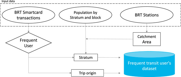
FIGURE 1. Frequent transit users database development framework.

3.1 Data Input and Pre-Processing

We used Bogota’s BRT smartcard data of individual transactions from January 1, 2020, to October 12, 2020. A transaction is automatically recorded when a smartcard approaches a reader device at the BRT station entrance. A transaction record contains the date and time, station name, entry point (for stations with multiple entry points), the fare, card type, and a unique identifying number. The unique identifying number links subsequent transactions made by the same card. In total, the dataset has more than 247 million transactions representing about 7.5 million unique smartcards (Transmilenio S.A., 2020b). We also used the official strata classification dataset, a shapefile containing more than 45,000 blocks with the stratum classification (Secretaría Distrital de Planeación Bogotá, 2020) and the block-level population extracted from the official census website (DANE, 2018).

We pre-processed smartcard data to obtain an individual’s transit travel sequence. We defined a transit travel sequence as all transactions registered by the same card ID. However, travel sequences may have double tap-ins or internal transfers within the system that need to be removed from the analysis. Consecutive transactions made in the same station by the same card within 30 min were assumed to be only one transaction. We also eliminated internal transfers. For example, some feeder stops are not located in the station but a nearby location. In these cases, users need to tap-in when they exit the feeder route stop and tap-in again when they enter the main station; however, this is only one transaction. We also eliminated transactions in “Virtual Stations” as they do not correspond to any physical location. One user may use multiple smartcards, or multiple users may use a single smartcard; however, the data set does not distinguish between the two. Therefore, we assumed that one card represents a unique user. Similar assumptions have been made in other smartcard data studies (Zhao et al., 2018).

We used the boarding stations and entry points to differentiate transactions of multiple services. Stations with feeder or intercity connections have designated entry points to ensure payment when entering a BRT station. Therefore, a BRT station can have walking, feeder, and intercity entry points, and each transaction is classified accordingly.

3.2 Frequent Users

The objective of separating frequent and non-frequent users is to distinguish transit travel sequences with enough information to infer their transit travel behavior. Users who do not have enough information may be sporadic users or visitors who use the system for a short amount of time. To compare individuals before and after the lockdowns, the selection of frequent users considered the transactions between January 1, 2020, and March 8, 2020.

To determine frequent users, we characterized each transit travel sequence with three variables: 1) total number of transactions, 2) number of active days, and 3) average transactions per active day. A distribution density plot for each variable is shown in Figure 2. As expected, the number of transactions decreases exponentially (Figure 2A). The distribution of the number of active days suggests that most unique transit users are sporadic (Figure 2B). Additionally, the distribution of the number of transactions per active day falls after five, suggesting that most people have fewer than five transactions a day on average (Figure 2C). To better understand the relationship among these variables, we plotted a joint distribution of the number of transactions versus the active days (Figure 2D). The plots show a linear relationship between the variables. However, there is a high concentration of sequences with fewer transactions and days of use that are more likely to be non-frequent users. We selected the cutoff point with the following rules: 1) the cutoff point should increase the variance of the joint distribution, and 2) the average values of the resulting distribution should be greater than the cutoff points. Figure 2E shows the joint distribution of the number of transactions and the active days with a cutoff point of 15 transactions and ten active days of use. The density distribution spreads along a line with slope one, suggesting an increased variance. The average values were higher than the cutoff points, suggesting that most infrequent transactions were filtered.

FIGURE 2

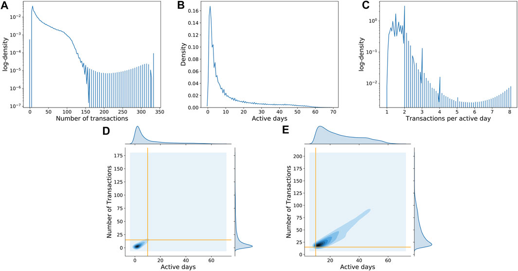
FIGURE 2. Transit travel sequence distributions. (A) Distribution of the number of transactions. (B) Distribution number of active days. (C) Distribution of the number of transactions per active day. (D) non-filtered joint distribution number of transaction and active days. (E) Filter joint distribution number of transaction and active days. Orange line represent the cutoff filter points at 10 active days, and 15 transactions.

Frequent transit users were classified as those unique identifier numbers that had transit travel sequences with more than 15 transactions, ten active days of use, fewer than 200 transactions, and average daily transactions fewer than five. After this filtering process, we remained with approximately 2 million users representing 70% of the total transactions. We only used these frequent users in our analysis.

Note that this process may have captured users who may not use transit every day or use transit frequently during a short period. While the inference of these users may be limited (e.g., we may not be able to infer a work location), these users tend to use the system in a certain way. For instance, someone who uses BRT for personal appointments or shopping will have the origin of their transactions most likely be linked to a regular location. Therefore, our study focuses not only on people who use transit frequently for commuting but also who use transit frequently for other activities.

3.3 Trip Origin—Home, Work and Other Location Inference

Transit travel sequences of frequent users reveal important information about each individual’s activity locations. The literature suggests a ruled-based approach that leverages the regularity of the transit travel sequence to infer locations such as home and work (Devillaine et al., 2012; El Mahrsi et al., 2014; Aslam et al., 2019). For example, the most frequent station is classified as the home station (Hasan et al., 2013; Flórez et al., 2017); or, if the time between two consecutive transactions is greater than a regular working session (e.g., 8 h), then it is a commuting trip (Chakirov and Erath, 2012; Long and Thill, 2015). These studies may also add external variables such as land use and household travel surveys to enrich the inference method (Chakirov and Erath, 2012; Long and Thill, 2015; Ordóñez Medina, 2018). Han and Sohn (2016) also suggests using continuous hidden Markov models to identify clusters in the smartcard data population and use this information to infer home and work locations. However, they tested their methodology with two days of observation.

The purpose of this section is to describe the methods used in this study to infer home and work locations. We also classified transactions at other locations as “other.” For simplicity, we used a similar set of rules as Long and Thill (2015). We adjusted some of the rules to reflect that our data set only contains tap-in information. We used the following rules to infer the activity locations:

• Home: Most common first transaction of the day before noon.

• Work: Most common transaction such that difference between consecutive transaction in the same day is greater than 6 h.

• Other: Transactions in any other station that are not classified as home or work.

Note that some transit sequences may have only one transaction a day or consecutive trips in the same day with less than 6 h difference. For these users, a work location was not inferred. They could potentially be less frequent riders that use the BRT for discretionary activities, and therefore these transactions were classified as other.

3.4 Catchment Areas

The catchment area of a BRT station is its area of influence. We assumed that each frequent transit rider in our processed database lives within the catchment area of their inferred home station. From the HTS, we estimated that 89% of the transit users live within the catchment areas and 87% access the BRT by walking. Only 5.9 and 3.8% access the station by other bus services and informal transit, respectively. Additionally, from the smartcard data, only 7.7% of the home location transactions are identified as transfers from other bus services that are not the feeder routes. These percentages validate that our assumption is a reasonable approximation of reality.

To estimate a catchment area, we followed these principles:

• The area of influence is a buffer with the maximum walking distance a person is willing to walk to access mass public transit.

• Catchment areas of different stations do not overlap.

• Only feeder routes will add to the catchment area outside the maximum walking distance.

The maximum walking distance to a BRT station is estimated from the 2019 HTS. From the survey, we filtered respondents that mention BRT as a transportation mode. We extracted the walking access and egress time from home to BRT station. From the distributions, 90% of the respondents reported access walking time less than 20 min. We assumed an average walking speed of 4.5 km/h, representing a maximum walking distance of 1500 m. This distance is more likely to correspond to a Manhattan distance. However, we created the buffer with a Euclidean distance. To convert the Manhattan distance to a Euclidean distance, we used the fact that the sum of the squared legs for any right triangle corresponds to the hypotenuse squared. To simplify the conversion, we assumed an isosceles triangle; therefore, the corresponding Euclidean distance is $2c$, where c is the triangle’s leg. From the Pythagoras theorem, we also know that for any isosceles triangle, the hypotenuse is $\sqrt{2}\ast c$. Finally, the conversion coefficient is $\sqrt{2}/2$. Therefore, the distance to create the catchment area buffers is 1000 m. A similar radial distance for BRT stations catchment areas is suggested in Jiang et al. (2012). If two catchment areas covered the same point, we assigned it to the closest station.

Feeder routes are a free service that amplify the catchment area of the station. Because it is a free service, users are not required to tap-in when they board a feeder bus, and thus, it is not possible to know the exact boarding location. However, stations have special entry points for feeder routes that are easy to identify. To account for these services, we defined the catchment area of a feeder route as a buffer of 500 m along the route, and considered it a different unit of analysis. Feeder route information did not include feeder services at “Portal 20 de Julio”; therefore, transactions from feeder lines at this station were excluded from the analysis. Figure 3 shows the catchment areas for both the stations and the feeder routes.

FIGURE 3

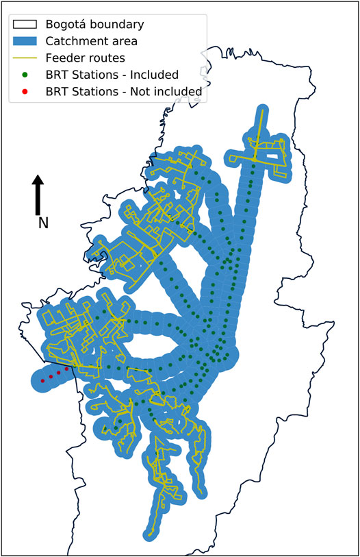
FIGURE 3. BRT stations, feeder routes and catchment areas.

3.5 Stratum

To infer the stratum of a user, we estimated an s-dimensional probability vector $P_n\left(s\right)$ that reflects, for each station n, the probability that a frequent transit rider classified as living in that station’s catchment area belongs to a particular stratum s. The probability of station n having stratum s$\left[P_n\left(S=s\right)\right]$ depends on the population of stratum s within the catchment area of station n and the rate at which a strata s uses BRT $\left(rat{e}_s\right)$. The importance of the rate is that it capture strata heterogeneity in BRT use, which is critical for this study’s objective.

$P_n\left(S=s\right)=\frac{Po{p}_{n,s}\ast rat{e}_s}{{\displaystyle \sum _{j\subseteq S}Po{p}_{n,j}\ast rat{e}_j}}(1)$

To estimate $rat{e}_s$, we regressed the transactions per station for users for whom that station was classified as their home-station with respect to the population by stratum within the catchment area of a station. The form of this regression can be any generalized linear model for continuous or count variables as shown in Eq. 2. The rate is the average marginal effect, which can be understood as the change in the number of home-transactions for one increase in a given stratum population (Eq. 3).

$transactions=f\left(z,\theta \right)(2)$

$rat{e}_s=\frac{\partial transactions}{\partial {\theta }_s}(3)$

To estimate BRT use rates by strata, we used ordinary least square (OLS). Using OLS estimates, we obtained a similar stratum shares distribution as the negative binomial estimates and the 2019 HTS for a week in February. While the negative binomial model performs better in terms of the AIC, it resulted in two outlier stations (large catchment area and a small number of transactions), which disproportionately increased the error measures such as the root mean squared error (RMSE). By the central limit theorem, a normal distribution approximates a negative binomial distribution for large mean values (DasGupta, 2010), which is the case for this study (the average number of home transactions in the BRT system is 3,556 transactions per station/day). One advantage of OLS estimation is that it provides straightforward interpretability of the coefficients (e.g., the average marginal effect of a variable is its estimated coefficient). The implication of using this approximation is that we could potentially get negative prediction or fractional number; however, the objective of performing a regression is not to predict ridership but to capture the heterogeneity in the use of BRT by strata. Since we obtain a similar result with both regressions, we preferred the OLS estimate for its interpretability.

Equation 4 is the regression used to estimate the rates for each stratum. The dependent variable was the number of transactions per station corresponding to users where that station was classified as a home-station. The independent variables were the population by stratum in the catchment area. The estimated coefficients represent the average number of transactions per inhabitant of a given stratum, which we called the stratum transaction rate. Since strata five and six are just 5.3% of the population, we estimated a unique coefficient for this combined population segment.

$transactions={\theta }_0+rat{e}_1\ast po{p}_{stratum1}+\dots +rat{e}_{56}\ast po{p}_{stratum56}(4)$

In stable conditions, the stratum’s transaction rate would only vary for weekdays and weekends and during seasonal holidays. However, under highly dynamic conditions, this rate is likely to change daily. Thus, to estimate the impact of COVID-19 lockdowns in BRT use, we estimated the stratum’s transaction rate daily. Inter-city trips, including the trips from Soacha, are excluded from the analysis because strata information at the block level is only available in Bogota. Table 1 shows an example of the results for four different days (Monday, Wednesday, Saturday, and Sunday). We noticed that coefficients for higher strata tend to be smaller in magnitude compared to lower strata. These results suggest that individuals from higher strata are less likely to use BRT, especially during the weekends. Note that these results do not include an intercept because it was statistically insignificant for all regressions.

TABLE 1

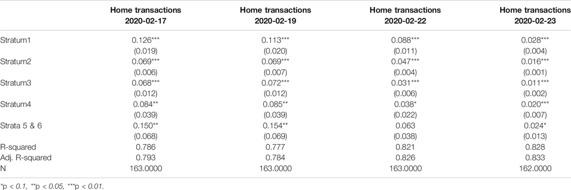
TABLE 1. Sample OLS estimation for strata inference. Samples days are Monday, Wednesday, Saturday and Sunday.

3.6 Validation

As with most inference methods and passive data, ground truth data is rarely available. Therefore it is not possible to validate these results from a statistical point of view. However, we can compare our results with the aggregate distributions from other data sets such as the household travel surveys and the census. This validation process also ensures that expected transit behavior can be observed, such as the bi-modal distribution of trips during a day, and that most inferred home locations are in residential areas.

To validate the proposed inference methods, we compared the results with expected distributions and distributions from other data sources. Figure 4A shows the distribution of the inferred home, work, and other locations for every frequent transit sequence. As expected, the distribution of home locations is mostly concentrated in the residential areas of the city perimeter. Similarly, work locations have a higher concentration in the downtown and the extended downtown of Bogota, where most jobs and universities are located. Lastly, locations classified as “other” are primarily distributed in both the downtown and residential areas, suggesting that “other” are potentially related to discretionary activities. To verify and strengthen our assumptions, we also plotted the transaction time for each location classification as shown in Figure 4B. As expected, the transaction time distribution for home locations peaks in the morning, which corresponds with the beginning of typical working/school hours. Likewise, the transaction time distribution for work locations peaks in the afternoon and coincides with the end of the typical working/school schedule. Transaction times for “other” locations are evenly distributed throughout the day, with some peak in the morning, midday and afternoon. Notice that we only constrained transactions before 12 P.M. to infer home locations; once inferred, every transaction in the home location is counted in the transaction distribution.

FIGURE 4

FIGURE 4. Validation plots. (A) Density distribution of home, work and other locations. (B) Transactions time distribution for home, work and other locations. (C) Distribution of population by strata (DANE, 2018) and BRT user by strata by proposed methodology. (D) Distribution of BRT users by strata (Secretaria Distrital de Movilidad, 2019) and proposed methodology.

To validate the strata inference, we compared the strata distribution of BRT users with the strata distribution of the population (DANE, 2018) (Figure 4C), and the 2019 HTS (Secretaria Distrital de Movilidad Bogotá, 2019) (Figure 4D). Our results show that the strata share closely matches the strata distribution as estimated from the 2019 HTS. From the HTS, we traced BRT trips with access modes different than walking. We found that they are more likely to be low-strata users, which may explain the underestimation of the share for strata one and overestimation of strata two.

Finally, with the methodology proposed in the study, we built a frequent transit users database with 2,011,067 unique users. Each user has a home and work location (when possible) and a strata probability distribution.

4 Results

This section presents the main findings and the statistical analysis to support them. We analyzed the trends by strata for the transaction reduction (%), the transactions per 1,000 people, and the radius of gyration (Rg). To calculate the transactions reduction on a given day, we compared it to the same day in the base week. For instance, any Tuesday is compared to the transactions of the Tuesday in the base week. We selected the week of February 17, 2020, as the base for these calculations as it is a typical week. We avoided using weeks in January because travel demand is usually atypical. We also avoided the first week of February as, by decree, the first Thursday of February is the day when travelers cannot use car or motorbike. Therefore, we expected transit demand to be higher than usual. Lastly, we defined the radius of gyration (Rg) as the average distance in kilometers reached by a person using BRT during a day, using the home station as an anchor, as shown in Eq. 5

$R{g}_n\left(t\right)=\sqrt{\frac{1}{S_{n,t}}{\displaystyle \sum _{i=1}^{S_{n,t}}d{\left(s_{\mathit{home},n},s_i\right)}^2}}(5)$

Where $R{g}_n\left(t\right)$ is the radius of gyration of individual n in the time t, $S_{n,t}$ is the number of stations visited by individual n in time period t, and $d\left(s_a,s_b\right)$ is a function that measures the Euclidean distance between station $s_a$ and station. Notice that $s_{\mathit{home},n}$ is the inferred home station of individual n.

For each of these variables (transaction reduction, transactions per 1,000 people, and the Rg), we fitted a line using OLS, where the dependent variable is a linear function of time, and the slope represents the trend. The main objective of this analysis is to use a statistical tool to test hypothesized significant differences in trends by strata. The z test for the difference in two estimated slopes is the one suggested in Paternoster et al. (1998), and we used a 95% confidence level. For each stratum, we fit a line in a defined period after the lockdowns and compared their slopes. If all slopes are statistically similar to each other, we conclude that the strata do not influence BRT demand during the COVID-19 pandemic. For the time variable, we added an indicator to differentiate between weekdays and weekends.

4.1 Transactions of Lower Strata Returned to Transit at a Faster Speed

The reduction in the number of transactions by stratum is shown in Figure 5. The plot shows the average transaction reduction over the last seven days to attenuate the weekend effect. We would expect a slight variation during the year under normal circumstances, as well as greater reductions during the holiday season in December—January and Easter. At the beginning of the lockdown, there was an initial sharp reduction in transactions of nearly 90% for middle and high strata, while for lower strata, the reduction was 85%. From the beginning of the general lockdown to the start of the sectorized lockdowns, there was a steady growth of transit use for all strata; however, the gap between lower and middle/higher strata increased to 15%, suggesting a more significant transit use growth rate for lower strata. A month after the end of the lockdown restrictions, this difference was approximately 20%. In Figure 5 we also see a drastic drop in demand after the sectorized lockdown that affected strata 1 and 2, but not other strata.

FIGURE 5

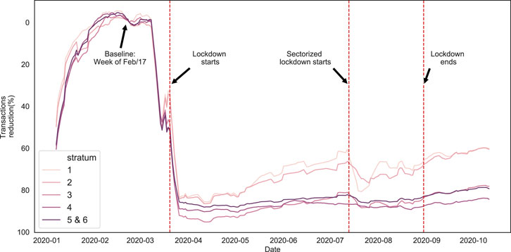
FIGURE 5. 7-days rolling average reduction of transactions (%) by strata. Reference is the week of February 17, 2020. Red dotted lines mark the start of the lockdown (Mar/20), the sectorized lockdown (Jul/13) and the end of the lockdown (Sep/01).

To test the difference in the slopes in Figure 5, we fit a line to each trend. To capture the difference between weekdays and weekends, we considered the daily reduction instead of the average reduction over the last seven days. We modeled two periods, the first between March 20 and July 13 and the second between September 01 and October 12. We did not model the period between the sectorized lockdowns as the trends for strata one and two are not linear. Table 2 shows the results for the first period. The slopes for all strata are positive and significantly different from zero. The small standard errors also suggest that these estimates are significantly different from each other. The slope can be interpreted as the daily return to transit rate. For strata one, this rate was 0.24%/day, which is five times higher than the rate for strata five and six. We also show that the reduction in transactions on the weekends was less severe than for weekdays. For instance, for strata five and six, the reductions in transactions on the weekends was 77.5% (100–7.568–14.939%), but for weekdays, the reduction was 92% (100–7.568%).

TABLE 2

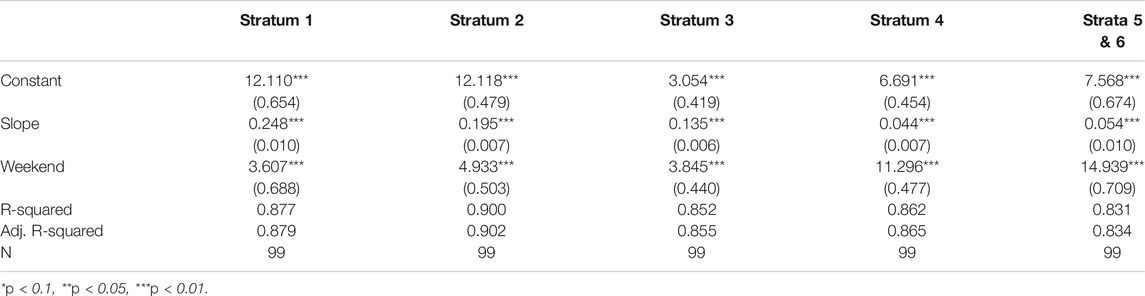
TABLE 2. OLS estimation. Dependent variable is the transactions reduction (%). Estimation period: Mar/20 to Jul/13 (99 days).

The results for the second period are shown in Table 3. The slope estimates are all positive and significant but not significantly different from each other. The constant estimate shows the difference in the transaction reductions between low strata (1–2) and middle/high strata (4–6) was between 15 and 25%. Since the slopes grow at the same rate, the disparity between low and middle/high strata remains stable in this period.

TABLE 3

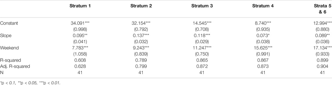
TABLE 3. OLS estimation. Dependent variable is the transactions reduction(%). Estimation period:Sep/01 to Oct/12 (41 days).

4.2 Transactions at “Other” Locations are Growing Faster Than Home and Work Locations

This section focuses on how the COVID-19 lockdowns have affected transactions by the location classification (home, work, and others). In Figure 6 we plotted the number of transactions per 1,000 people by transaction location and strata. This variable was selected to compare the behavioral change of transit use during the recovery period. As expected, strata 4 to 6 have low values for transactions per 1,000 people, and they are relatively constant until the end of the lockdowns. For strata one to three, the plot shows a drastic reduction at the beginning of the sectorized lockdowns for all transaction type. However, other strata only show a slight decrease. After the end of the lockdown restrictions, the plot suggests that transactions at “other” locations were growing faster than home and work trips for all strata, but this increase was steeper for strata one to three.

FIGURE 6

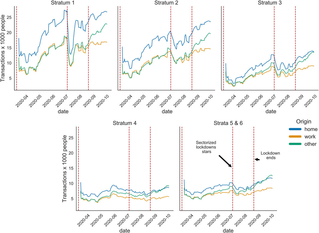
FIGURE 6. Transactions per thousand people by strata and location type in the recovery period only. Red dotted lines mark the start of the lockdown (Mar/20), the sectorized lockdown (Jul/13) and the end of the lockdown (Sep/01).

To test this last hypothesis, we fit these trends with a line to compare the value of the slopes. For this test, we only selected the data from September 1, through October 12. The results are shown in Table 4. The slopes are all positive and significant at the 95% level, except for work in strata one. For all strata, the slope for “other” transactions is greater than for home and work. However, for strata one to three, it is significantly steeper than for any other strata. Notice that for strata one, the slope for “other” is more than double the home transactions slope.

TABLE 4

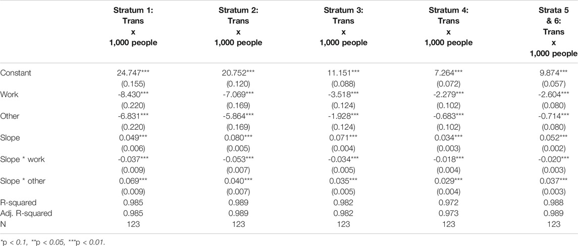
TABLE 4. OLS estimation. Dependent variable is the transactions per 1,000 population. For the categorical variable activity origin type, category home is the base. Estimation period: Sep/01 to Oct/12 (41 days), excluding weekends.

4.3 The Radius of Gyration Slightly Decreases for Lower Strata but Increases for Higher Strata

While other studies have shown that the Rg decreased about 50% after the initial lockdowns (Klein et al., 2020), our study shows that when measuring Rg only for users who continued using BRT in Bogota, their Rg slightly decreased for lower and medium strata and increased for higher strata, as shown in Figures 7 and 8. Specifically, the average Rg slightly decreasesfor strata one to three but significantly increases in other strata. For the sectorized lockdowns, the average Rg seems unaffected, but strata five and six have a decreasing trend.g. Typically, the Rg is calculated with GPS tracks collected regardless of mode. For the GPS case, it is possible to accurately measure an Rg of zero if a person stays at home, and therefore their observation is usually included in the average Rg estimation. As for our RG measure using public transit transactions data, the average Rg on a given day can only be calculated if an individual rides transit that day. Therefore, after the lockdown, our measure of Rg represents the average distance reached on public transit by users who continue using transit after the lockdowns.

FIGURE 7

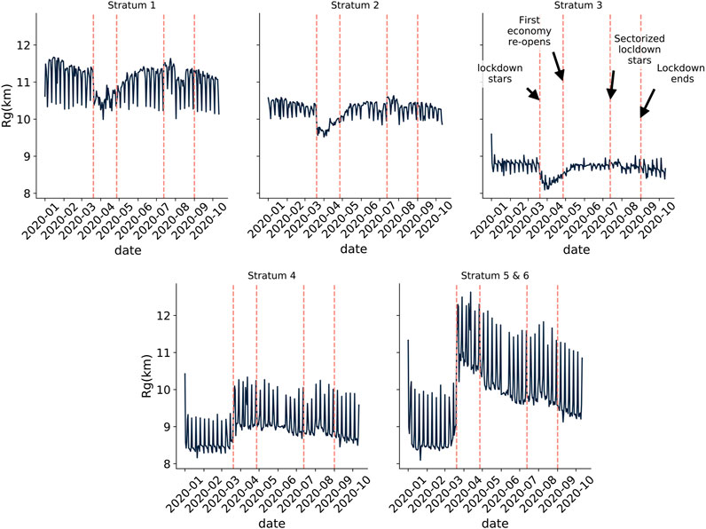
FIGURE 7. Average Radius of Gyration (Rg) in km by strata. Red dotted lines mark the start of the lockdown (Mar/20), the first economy re-opening (Apr/27), the sectorized lockdown (Jul/13) and the end of the lockdown (Sep/01).

FIGURE 8

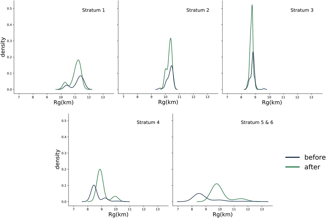
FIGURE 8. Distributions of Average Radius of Gyration (Rg) in km. Blue is the distribution before the lockdown. Green is the distribution after the first economy re-opening.

Unlike the analyses of transactions rates, the Rg is more stable for most strata, so fitting a line to the trend may not be appropriate because the slope is more likely to be zero. For this reason, we performed a two-sample t-test for mean comparison to test if Rg before and after the lockdown are significantly different. The null hypothesis is that the average Rg difference before and after the pandemic is equal to zero, and the alternative hypothesis is that it is different from zero. The after-lockdown data represents the days after the first day of the economy re-opening. We calculated the Welsh t-test and used the Satterthwaite formula for the degrees of freedom approximation; this procedure assumes that each sample variance is unequal. The results show that for strata two, we fail to reject the null hypothesis, and therefore, there is no significant difference in the average Rg before and after the lockdowns. For strata one and three, there is a slight but significant decrease of the Rg. For strata four to six, we reject the null hypothesis in favor of the alternative hypothesis and conclude that the average Rg is higher after the lockdown for this population. The results are shown in Table 5.

TABLE 5

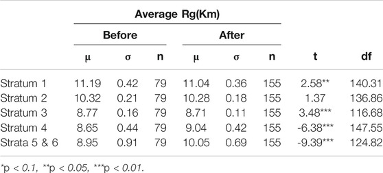
TABLE 5. Average Radius of Gyration in KM mean difference t-test. Before time period is Jan/01–Mar/20. After period is Apr/27–Oct/12.

5 Discussion

Our results show that strata one and two have different behavior than other strata and that middle and high strata behaved similarly during the pandemic. Lower strata had the least reduction in public transit use after the lockdowns and returned to transit more quickly. These results may show that low strata have a higher proportion of captive users who need public transportation to access jobs. In the context of Bogota, public transit captivity can be understood in two ways. First, lower strata have a low rate of vehicle ownership. According to the 2019 HTS, strata one and two have 95.5 and 137.7 vehicles per 1.000 people, respectively, while the same rate is 593.3 for strata six. Second, the spatial distribution of the strata in Bogota makes it challenging to switch to alternative modes such as walk or bike because low-income neighborhoods are further away from the downtown. Even bike ownership for lower-strata is lower than for higher-strata, with 111 bikes per 1.000 people for strata one and 319 bikes per 1.000 for strata six (Secretaria Distrital de Movilidad Bogotá, 2019). Middle and high strata not only have higher rates for personal and private vehicle ownership, but are also closer to job areas. Therefore, it is easier to switch to sustainable modes such as walking and biking. These results could also be influenced by the fact that new bike lines are highly concentrated in the middle and higher stratum; these bike lanes were implemented to give transit users better and safer options to commute during the COVID-19 pandemic.

The sectorized lockdowns also had different impacts by strata. The first set of neighborhoods affected by the lockdown were dense job areas and low strata neighborhoods, explaining the higher drop in strata one and two. During this first phase, reduction rates for stratum one were similar to middle and higher strata. However, as the restrictions eased for those neighborhoods, stratum one quickly returned to levels similar to those right before the sectorized lockdowns, while transactions in middle and higher strata remained low. Lockdowns in other phases seem to have had little effect on the BRT demand. As the economy re-opens, the number of transactions at home and work locations follows a similar trend. However, the growth rate for “other” transactions increased for every stratum. The increase of transactions in “other” locations could be influenced by the eased restrictions and the fact that public transit continued to operate with 100% of its fleets despite its remains with low occupancy. As the BRT has good connectivity and accessibility, the population may have used it more for other activities outside work.

As for the Rg, the distance reached on public transit by lower and middle strata decreased only slightly after the lockdowns. This result shows that those users who continued using transit are reached similar destinations before and after the lockdowns. These trends do not seem to be affected by the sectorized schema. However, for higher strata, the Rg increased during the lockdowns. This result may show that most of the low short-distance high strata BRT trips made by individuals in the high strata were replaced by other modes, while these individuals continued using BRT for long-distances trips. This is consistent with findings in (João Filipe Teixeira and Lopes, 2020). Strata five and six also showed a decline in the average Rg, which might have been influenced by the increased transactions in “other” locations. One contribution of this study is the calculation of the Rg specific to a transportation mode, in this case, the BRT. Other studies calculate the Rg based on the visited locations regardless of the transportation mode used to access those locations. These studies showed a significant drop in the Rg, but they did not compare it for the individuals who remained traveling during the COVID-19 pandemic. For transit operation and even for other transportation services, this information is vital to adapt the supply to current demand needs.

Our study highlighted that the reduction in demand for the BRT system was not distributed equally among strata. Therefore, fleet operations should not remain equal to the pre-lockdown schedules. To promote equity in the transit services, transit agencies need to shift resources to where they are most needed, such as location used by vulnerable populations that solely depend on transit. A more in-depth analysis of the BRT origin-destination pairs may help identify which pairs to prioritize based on the strata, the transaction volume, and the activity type. While our results show a differential impact based on strata, the methodology only captures frequent users before the pandemic and analyzes their trends after the pandemic. We did not account for infrequent users that have become frequent users after the lockdowns, as we did not have a reference point for them. Additionally, while we assumed that different strata have different rates of taking transit, we did not consider that longer distances to BRT stations may reduce the probability to take BRT. As a result, the current methodology may be overestimating the representation of BRT use in the edges of BRT stations’ catchment areas. However, these results provide a general understanding of how transit demand is shifting during the COVID-19 pandemic for different strata.

6 Limitations and Future Work

The current methodological approach to infer home and work location did not consider work instability. We defined work instability as a worker with varying working locations such as construction workers or people in the informal job market, which is likely to affect the results for low strata. For instance, one user can have both work, and study locations, but the methodology will only capture one or the other. Further research in this area may help us understand and classify more complex tours. We did not consider home or work change. This assumption is particularly important because the COVID-19 lockdowns may have also impacted relocation rates. However, data on home and work re-locations before the 2020 is not available as a baseline. Another limitation is that, we assumed that the probability vector of a transaction belonging to one stratum depends only on the strata distribution within the catchment area and the rates of transit use for each stratum. We did not consider other factors such as distance, which may give greater weight to blocks closer to the stations. Moreover, frequent users were estimated using data pre-lockdown data only. We did not account users that may have become frequent and active after the lockdowns. We also assumed that catchment areas are the only source of strata variation, however it is possible that some home transactions may fall outside the transit catchment area, given some informal services that are used as feeder routes. For instance, users outside a given catchment area may use bicitaxis or cars to reach their homes. Finally, information on informal transit was not available, and therefore was not accounted for in this study.

7 Conclusion

We classified transactions of frequent users by strata using a probability vector, which is a function of the rate of BRT use and the population in the catchment area of the station. This classification showed a similar aggregate strata distribution as the 2019 HTS, which validated our inference methodology. The results from this study showed a differential impact of the COVID-19 pandemic on BRT use by strata. Lower strata showed the least reduction of transit use compared to middle and higher strata. At the beginning of the lockdown period, lower strata returned to transit more quickly than any other stratum. By the end of the lockdown restrictions, the number of trips to “other” locations was significantly higher than those of work trips, which adds extra challenges to transit operators. This study also showed that transit users in lower strata were reaching similar destinations as before the lockdown, as measured by Rg. However, for higher strata, the average Rg increased during the lockdown, suggesting that they may have replaced their shorter trips with other modes but kept using BRT for their longer trips. This study’s results can help transit agencies better allocate resources to improve the level of service and accessibility to both home and work locations for vulnerable populations.

Data Availability Statement

The data and code supporting the conclusion of this article is available at https://github.com/jdcaicedo251/transmilenio-covid.git.

Author Contributions

JC, JW, and MG contributed to the conception and design of the study. JC organized the database. JC performed the statistical analysis. JC wrote the first draft of the manuscript. JC, JW, and MG contributed to manuscript revision, read, and approved the submitted version.

Conflict of Interest

The authors declare that the research was conducted in the absence of any commercial or financial relationships that could be construed as a potential conflict of interest.

References

Almlöf, E., Rubensson, I., Cebecauer, M., and Jenelius, E. (2020). Who Is Still Travelling by Public Transport during COVID-19? Socioeconomic Factors Explaining Travel Behaviour in Stockholm Based on Smart Card Data. SSRN J. doi:10.2139/ssrn.3689091

CrossRef Full Text | Google Scholar

Alon, T., Doepke, M., Olmstead-Rumsey, J., and Tertilt, M. (2020). National Bureau of Economic Research. doi:10.3386/w26947The Impact of COVID-19 on Gender Equality Working Paper 26947. Cambridge, MA, USA.

CrossRef Full Text | Google Scholar

Aslam, N. S., Cheng, T., and Cheshire, J. (2019). A High-Precision Heuristic Model to Detect Home and Work Locations from Smart Card Data. Geo-spatial Inf. Sci. 22, 1–11. doi:10.1080/10095020.2018.1545884

CrossRef Full Text | Google Scholar

Astroza, S., Tirachini, A., Hurtubia, R., Carrasco, J. A., Guevara, A., Munizaga, M., et al. (2020). Mobility Changes, Teleworking, and Remote Communication during the COVID-19 Pandemic in Chile. Findings. doi:10.32866/001c.13489

CrossRef Full Text | Google Scholar

Bocarejo S., J. P., and Oviedo H., D. R. (2012). Transport Accessibility and Social Inequities: a Tool for Identification of Mobility Needs and Evaluation of Transport Investments. J. Transport Geogr. 24, 142–154. doi:10.1016/j.jtrangeo.2011.12.004

CrossRef Full Text | Google Scholar

Brough, R., Freedman, M., and Phillips, D. (2020). Understanding Socioeconomic Disparities in Travel Behavior during the COVID-19 Pandemic. SSRN J. doi:10.2139/ssrn.3624920

CrossRef Full Text | Google Scholar

Camporeale, R., Caggiani, L., Fonzone, A., and Ottomanelli, M. (2017). Quantifying the Impacts of Horizontal and Vertical Equity in Transit Route Planning. Transportation Plann. Tech. 40, 28–44. doi:10.1080/03081060.2016.1238569

CrossRef Full Text | Google Scholar

Cantillo-García, V., Guzman, L. A., and Arellana, J. (2019). Socioeconomic Strata as Proxy Variable for Household Income in Transportation Research. Evaluation for Bogotá, Medellín, Cali and Barranquilla. Dyna 86, 258–267. doi:10.15446/dyna.v86n211.81821

CrossRef Full Text | Google Scholar

Chakirov, A., and Erath, A. (2012). Activity Identification and Primary Location Modelling Based on Smart Card Payment Data for Public Transport.

Google Scholar

DANE (2018). Anílisis Geoespacial del CNPV 2018. Available at: https://geoportal.dane.gov.co/geovisores/territorio/analisis-cnpv-2018/ (Accessed 06 09, 2020).

Google Scholar

DANE (2015). Metodologia de estratificacion socioeconomica urbana para servicios publicos domiciliarios - enfoque conceptual. Available at: https://www.dane.gov.co/files/geoestadistica/estratificacion/EnfoqueConceptual.pdf (Accessed 03, 2021).

Google Scholar

DasGupta, A. (2010). “Normal Approximations and the Central Limit Theorem” in Normal Approximations and the Central Limit Theorem. In Fundamentals of Probability: A First Course. (Springer), 213–242. doi:10.1007/978-1-4419-5780-1_10

CrossRef Full Text | Google Scholar

Delmelle, E. C., and Casas, I. (2012). Evaluating the Spatial Equity of Bus Rapid Transit-Based Accessibility Patterns in a Developing Country: The Case of Cali, Colombia. Transp. Policy 20, 36–46. doi:10.1016/j.tranpol.2011.12.001

CrossRef Full Text | Google Scholar

Devillaine, F., Munizaga, M., and Trépanier, M. (2012). Detection of Activities of Public Transport Users by Analyzing Smart Card Data. Transportation Res. Rec. 2276, 48–55. doi:10.3141/2276-06

CrossRef Full Text | Google Scholar

Dueñas, M., Campi, M., and Olmos, L. (2020). Working Papers 62. Red Investigadores de Economía.Changes in Mobility and Socioeconomic Conditions in Bogotá City during the COVID-19 Outbreak. arXiv preprint arXiv:2008.11850.

Google Scholar

El Mahrsi, M., Côme, E., Baro, J., and Oukhellou, L. (2014). Understanding Passenger Patterns in Public Transit through Smart Card and Socioeconomic Data: A Case Study in Rennes, france in ACM SIGKDD Workshop on Urban Computing.

Google Scholar

Fairlie, R. (2020). National Bureau of Economic Research. doi:10.3386/w27462The Impact of COVID-19 on Small Business Owners: The First Three Months after Social-Distancing Restrictions Working Paper 27462. Cambridge, MA.

CrossRef Full Text | Google Scholar

Flórez, M., Jiang, S., Li, R., Mojica, C., Ríos, R., and González, M. (2017). Measuring the Impacts of Economic Well Being in Commuting Networks - a Case Study of Bogota, colombia.

Google Scholar

Han, G., and Sohn, K. (2016). Activity Imputation for Trip-Chains Elicited from Smart-Card Data Using a Continuous Hidden Markov Model. Transportation Res. B Meth. 83, 121–135. doi:10.1016/j.trb.2015.11.015

CrossRef Full Text | Google Scholar

Hasan, S., Schneider, C. M., Ukkusuri, S. V., and González, M. C. (2013). Spatiotemporal Patterns of Urban Human Mobility. J. Stat. Phys. 151, 304–318. doi:10.1007/s10955-012-0645-0

CrossRef Full Text | Google Scholar

Huang, J., Wang, H., Fan, M., Zhuo, A., Sun, Y., and Li, Y. (2020). “Understanding the Impact of the COVID-19 Pandemic on Transportation-Related Behaviors with Human Mobility Data,” in Proceedings of the 26th ACM SIGKDD International Conference on Knowledge Discovery & Data Mining. New York (NY, USA: Association for Computing Machinery), KDD ’20, 3443–3450. doi:10.1145/3394486.3412856

CrossRef Full Text | Google Scholar

Institute for Transportation and Development Policy (2020). Post-pandemic, Chinese Cities Gradually Reopen Transport Networks. Available at: https://www.itdp.org/2020/03/26/post-pandemic-chinese-cities-gradually-reopen-transport-networks/ (Accessed June 15, 2020).

Google Scholar

Inter-American Development Bank (2020). Coronavirus Impact Dashboard. Available at: https://www.iadb.org/en/topics-effectiveness-improving-lives/coronavirus-impact-dashboard (Accessed June 15, 2020).

Google Scholar

Jiang, Y., Christopher Zegras, P., and Mehndiratta, S. (2012). Walk the Line: Station Context, Corridor Type and Bus Rapid Transit Walk Access in Jinan, China. J. Transport Geogr. 20, 1, 14. doi:10.1016/j.jtrangeo.2011.09.007

CrossRef Full Text | Google Scholar

Klein, B., LaRocky, T., McCabey, S., Torresy, L., Privitera, F., Lake, B., et al. (2020). Assessing Changes in Commuting and Individual Mobility in Major Metropolitan Areas in the united states during the Covid-19 Outbreak 29.

Google Scholar

Long, Y., and Thill, J.-C. (2015). Combining Smart Card Data and Household Travel Survey to Analyze Jobs-Housing Relationships in Beijing. Comput. Environ. Urban Syst. 53, 19–35. doi:10.1016/j.compenvurbsys.2015.02.005

CrossRef Full Text | Google Scholar

MinSalud (2020). Determinantes sociales: elementos a tener en cuenta para la toma de decisiones en el país 2020. Available at: https://www.minsalud.gov.co/Paginas/Determinantes-sociales-elementos-a-tener-en-cuenta-para-la-toma-de-decisiones-en-el-pais.aspx (Accessed March 15, 2020).

Google Scholar

Molloy, J., Tchervenkov, C., Schatzmann, T., Schoeman, B., Hintermann, B., and Axhausen, K. W. (2020). Mobis-Covid19/29. Results as of 30/11/2020 (Second Wave). doi:10.31124/advance.13689751.v1

Google Scholar

Munoz-Raskin, R. (2010). Walking Accessibility to Bus Rapid Transit: Does it Affect Property Values? the Case of Bogotá, Colombia. Transp. Policy 17, 72–84. doi:10.1016/j.tranpol.2009.11.002

CrossRef Full Text | Google Scholar

Ordóñez Medina, S. A. (2018). Inferring Weekly Primary Activity Patterns Using Public Transport Smart Card Data and a Household Travel Survey. Trav. Behav. Soc. 12, 93–101. doi:10.1016/j.tbs.2016.11.005

CrossRef Full Text | Google Scholar

Orro, A., Novales, M., Monteagudo, Á., Pérez-López, J.-B., and Bugarín, M. R. (2020). Impact on City Bus Transit Services of the COVID-19 Lockdown and Return to the New Normal: The Case of A Coruña (Spain). Sustainability 12, 7206. doi:10.3390/su12177206

CrossRef Full Text | Google Scholar

Pappalardo, L., Simini, F., Barlacchi, G., and Pellungrini, R. (2019). Scikit-Mobility: a Python Library for the Analysis, Generation and Risk Assessment of Mobility Data. doi:10.1145/3308560.3320099

CrossRef Full Text | Google Scholar

Paternoster, R., Brame, R., Mazerolle, P., and Piquero, A. (1998). Using the Correct Statistical Test for the Equality of Regression Coefficients. Criminology 36, 859–866. doi:10.1111/j.1745-9125.1998.tb01268.x

CrossRef Full Text | Google Scholar

Pérez-Messina, I., Graells-Garrido, E., Lobo, M. J., and Hurter, C. (2020). Modalflow: Cross-Origin Flow Data Visualization for Urban Mobility. Algorithms 13, 298. doi:10.3390/a13110298

CrossRef Full Text | Google Scholar

Secretaria Distrital de Movilidad Bogotá (2019). Household Travel Survey 2019. Available at: https://www.simur.gov.co/portal-simur/datos-del-sector/encuestas-de-movilidad/ (Accessed March 15, 2020).

Google Scholar

Secretaria Distrital de Planeación Bogotá (2020). Rutas Zonales del SITP. Available at: https://datosabiertos.bogota.gov.co/dataset/manzana-estratificacion-bogota-d-c (Accessed June 13, 2020).

Google Scholar

Sumner, A., Hoy, C., and Ortiz-Juarez, E. (2020). Estimates of the Impact of COVID-19 on Global Poverty. Unuwider 2020, 1–9. doi:10.35188/UNU-WIDER/2020/800-9

CrossRef Full Text | Google Scholar

Teixeira, J. F., and Lopes, M. (2020). The Link Between Bike Sharing and Subway Use During the COVID-19 Pandemic: The Case-Study of New York's Citi Bike. Transportation Res. Interdiscip. Perspect. 6, 100166. doi:10.1016/j.trip.2020.100166

CrossRef Full Text | Google Scholar

The International Association of Public Transport (2020). Management of Covid-19 Guidelines for Public Transport Operators. Available at: https://www.uitp.org/publications/management-of-covid-19-guidelines-for-public-transport-operators/ (Accessed February, 2020).

Google Scholar

TransitApp (2020a). How Coronavirus Is Disrupting Public Transit. Available at: https://transitapp.com/coronavirus (Accessed June 15, 2020).

Google Scholar

TransitApp (2020b). Who’s Left Riding Public Transit? A COVID Data Deep-Dive. Available at: https://medium.com/transit-app/whos-left-riding-public-transit-hint-it-s-not-white-people-d43695b3974a (Accessed May 30, 2020).

Google Scholar

Transmilenio S.A. (2020a). Report. Estadísticas de oferta y demanda del sistema integrado de transporte público - sitp - febrero. Available at: https://www.transmilenio.gov.co/publicaciones/151672/estadisticas-de-oferta-y-demanda-del-sistema-integrado-de-transporte-publico-sitp-febrero-2020/ (Accessed March, 2021).

Google Scholar

Transmilenio S.A. (2020b). Validaciones Tarjetas Tu Llave. Available at: https://datosabiertos-transmilenio.hub.arcgis.com (Accessed October 13, 2020).

Google Scholar

Wang, D., He, B. Y., Gao, J., Chow, J. Y. J., Ozbay, K., and Iyer, S. (2020). Impact of COVID-19 Behavioral Inertia on Reopening Strategies for new york City Transit. CoRR abs/2006.13368

Google Scholar

Wilbur, M., Ayman, A., Ouyang, A., Poon, V., Kabir, R., Vadali, A., et al. (2020). Impact of COVID-19 on Public Transit Accessibility and Ridership.

Google Scholar

World Health Organization (2020). Supporting Healthy Urban Transport and Mobility in the Context of Covid-19. Publication. Available at: https://www.who.int/publications/i/item/9789240012554 (Accessed February 11, 2020).

Google Scholar

Zhao, Z., Koutsopoulos, H. N., and Zhao, J. (2018). Individual Mobility Prediction Using Transit Smart Card Data. Transportation Res. C: Emerging Tech. 89, 19–34. doi:10.1016/j.trc.2018.01.022

CrossRef Full Text | Google Scholar