 P. Hong1
 H. P. Hong2*
- 1School of Civil Engineering and Architecture, Nanchang Hangkong University, Nanchang, China
- 2Department of Civil and Environmental Engineering, University of Western Ontario, London, ON, Canada
The time history analysis is used to estimate the peak responses of structures subjected to stationary and nonstationary winds. The time histories of the fluctuating wind processes at multiple points can be simulated based on the spectral representation method for given target auto and cross power spectral density (PSD) functions. As the number of the processes of interest increases, the computation time for the simulation increases drastically. For the stationary homogeneous or nonhomogeneous wind fields, this problem can be overcome by using the frequency-wavenumber PSD function to simulate the stochastic propagating waves or fields. In the present study, a technique to simulate the amplitude modulated and frequency modulated nonstationary and nonhomogeneous stochastic propagating wind fields is presented. The technique relies on representing the nonstationary wind velocity by amplitude modulating a process that is time transformed from a stationary process. It is based on the established relations between the PSD functions of the nonstationary and of the stationary wind velocity. Simple to use and implement equations to carry out the simulation for one-dimensional line wind velocity field and two-dimensional nonstationary and nonhomogeneous wind velocity field are presented. The use of the developed technique and its adequacy is illustrated through numerical examples.
Introduction and Background
Structures such as tall buildings, long bridges, and wind turbines are sensitive to wind actions (Simiu and Scanlan, 1996; Strommen, 2010). The time history of wind velocity at a point on a structure can be represented by the sum of the mean and fluctuating wind components. The fluctuating winds can be characterized by using the power spectral density (PSD) function such as the Davenport spectrum, Kaimal spectrum, and von Karman spectrum. A common characteristic of these spectra is that they can be expressed in terms of reduced frequency or Monin coordinate, which is proportional to the turbulence length scale and inversely proportional to the mean wind velocity. The relation between two fluctuating wind velocity time histories at two spatial points is modelled using the coherence function (Davenport, 1967; Mann, 1994; Krenk, 1996; Simiu and Scanlan, 1996; Solari and Piccardo, 2001; Peng et al., 2018).
The estimation of the structural responses to the wind loading can be carried out in the frequency domain or time domain. It is well recognized that the use of the frequency domain approach to estimate the peak responses for simple structures can be very efficient for linear elastic systems (Simiu and Scanlan, 1996). The use of the time domain approach becomes increasingly popular because of the availability of powerful time-history structural analysis software and computer science and engineering advances. The use of time-domain analysis also facilitates the evaluation of nonlinear inelastic structural responses and reliability by considering wind loading (Vickery, 1970; Hong, 2004; Hong, 2016) or earthquake loading (e.g., Hong and Hong, 2007). For the time history analysis, the synthetic wind velocity fields need to be generated. The simulation of wind velocity can be carried out using one of the several available methods, including the spectral representation method (SRM) (Shinozuka and Jan, 1972; Li and Kareem, 1991; Shinozuka and Deodatis, 1996; Di Paola, 1998; Spanos and Zeldin, 1998; Huang and Chen, 2009), auto-regressive moving-average (ARMA) model (Samara et al., 1985); the empirical mode decomposition (Xu and Chen, 2004); proper orthogonal expansion (Chen and Kareem, 2005; Carassale et al., 2007; Solari et al., 2007), and application of wavelet transform (Gurley and Kareem, 1999).
For the fluctuating wind modelled as a stationary process defined by its PSD function, the most popular method to simulate the time histories of wind velocity is SRM. As the PSD function of fluctuating wind velocity is a function of the mean wind velocity (Simiu and Scanlan, 1996), the PSD function becomes dependent on both the frequency and time. In such a case, the coupling of time and frequency in the PSD function is such that the factorization of the time-frequency-dependent PSD function as a function of time and a function of frequency could be difficult (Hong, 2016) if it is not impossible. To simplify the task of simulating the nonstationary wind velocity, some researchers (e.g., Chay et al., 2006; Chen and Letchford, 2007; Li et al., 2017) assumed that the square root of the whole evolutionary PSD (EPSD) function can be treated as the amplitude modulation function. The assumption is very practical but may not agree with the requirement that the amplitude modulation for an evolutionary process must be a slowly varying function (Priestley, 1965). Hong (2016) proposed the use of a uniformly amplitude modulated and frequency modulated (AM/FM) process to model nonstationary fluctuating wind. In other words, the nonstationary fluctuating wind velocity is represented by amplitude modulating a process that is nonlinearly time transformed from a stationary process. For the fluctuating winds at multiple points in space, this model describes the fluctuating winds with advection according to their corresponding time-varying mean wind velocity.
Given a PSD or EPSD matrix of the fluctuating winds at multiple points in space, the time histories of turbulent winds at these points can be modelled using SRM (Shinozuka and Deodatis, 1996). As the number of the processes defined by the matrix increases, the use of SRM for the simulation of the processes is inefficient since it involves the decomposition of the matrix at many frequencies and the application of the fast Fourier transform (FFT) to improve the computational efficiency may not be possible unless approximations are considered (Li et al., 2017).
Rather than simulating nonstationary wind processes at multiple points, Deodatis and Shinozuka (1989) proposed an efficient technique to simulate the stochastic waves (or fields) for a given frequency-wavenumber PSD (FW-PSD) function, which is an extension of SRM (Di Paolo, 1998). The use of the FW-PSD function based simulation for multi-dimensional random field is much more efficient than the use of multiple points based simulation for vector processes since the former avoids the decomposition of the power spectral density function at many frequencies. For the simulation of the one-dimensional homogeneous wind field, Benowitz and Deodatis (2015) showed that the FW-PSD function could be obtained from the auto PSD and cross PSD (XPSD) Functions of homogeneous fluctuating winds for two points in space. They modified the technique given in Deodatis and Shinozuka (1989) by using FFT to gain additional computational efficiency and showed the adequacy of the simulated wind field for a bridge deck represented as a horizontal line-like exposed structure. Chen et al. (2018) and Song et al. (2018) investigated the simulation of homogeneous and nonhomogeneous wind fields in two spatial dimensions by considering that the inhomogeneity is originated from the height varying mean wind velocity. In their study, the coherence is considered to depend only on the separations in the horizontal and vertical directions or Euclidian distance but independent of the coordinate of the points in space. It is noted that the simulation of nonstationary and nonhomogeneous wind fields by using the FW-PSD function has not been addressed in the literature. The nonstationary fluctuating wind could arise from time-varying mean wind speed due to thunderstorm events, while the inhomogeneity could be caused by the topographic effects or characteristics of the winds that vary with the height or the coherence that depends on the spatial coordinate and separation. These problems are often encountered in evaluating wind-induced responses of bridges (King, 2003), transmission tower and tower-line systems (Momomura et al., 1997; Yang and Hong 2016; Yang et al., 2017), and tall buildings (Irwin, 2009).
The main objective of the present study is to develop a simple technique to simulate the AM/FM and nonhomogeneous stochastic propagating wind velocity fields. It is considered that the nonstationary fluctuating winds at multiple points are represented by AM/FM processes (Hong, 2016). The remaining sections of the present study are organized as follows. Simulation of an Amplitude Modulated Evolutionary Stochastic Field section summarizes the essential theoretical formulation given in Deodatis and Shinozuka (1989) to simulate an amplitude modulated evolutionary stochastic propagating waves or fields. Simulation of Nonstationary and Nonhomogeneous Propagating Stochastic Field section describes the theoretical development leading to the formulation for simulating AM/FM and nonhomogeneous propagating stochastic fields. Numerical Examples section presents the numerical example applications.
Simulation of an Amplitude Modulated Evolutionary Stochastic Field
Consider that a stochastic propagating wave or field in time and n-dimensional space,
where
The FW-PSD function of
Based on this amplitude modulated stochastic field model, Deodatis and Shinozuka (1989) (see also Shinozuka and Deodatis, 1996) showed that
where
Simulation of Nonstationary and Nonhomogeneous Propagating Stochastic Field
Adopted Time-Frequency-Dependent Power Spectral Density Function
The application of Eq. 3 to simulate the wind field is simple, provided that
where S0f(f) denotes the PSD function, f (Hz) is the frequency, A0, B0, a0, b0, and c0 are model parameters,
Based on the type of PSD function shown in Eq. 5 such as the Kaimal spectrum and the concept of time transformation (i.e., frequency modulation) (Yeh and Wen, 1990), the AM/FM model for the nonstationary fluctuating winds proposed in Hong (2016) is adopted in the following. The adopted model considers that the wind velocity is represented by the sum of the mean wind velocity U(pj, t) and fluctuating wind velocity u(pj, t) at a point in space pj, where pj = (x1j, x2j) in which x1j and x2j represent the coordinates of the horizontal and vertical axes, respectively. u(pj, t) is given by,
and,
where the time-varying standard deviation of the nonstationary process
where A0 in this equation is a normalization constant to ensure that the integration of
which represents the normalized Kaimal spectrum with the variance equal to one.
The nondimensional quantity τj viewed as the “time” variable could also be viewed as a “space” variable, depending on the preference of the user. Viewing as the “space” variable, the wind in this model is treated as a frozen wind with its time variation described by advecting the wind with a constant mean wind velocity in the τ-domain. It is homogeneous except for amplitude modulation. The PSD function of
where
In order to deal with multiple processes, each representing the wind velocity at a spatial point, define two stationary processes,
in which
where
This function differs from the lagged coherence function given by Davenport (1967) (see also Simiu and Scanlan, 1996; Hong, 2016) on how the mean wind speed is averaged. For fixed points, the lagged coherence decreases as the mean wind velocity increases. The lagged coherence also decreases with increasing frequency or separation. The vertical coordinate plays a minor role in controlling the lagged coherence.
Formulation for Simulating AM/FM and Nonhomogeneous Propagating Wind Field
As
where the use of the one-sided PSD function of
The FW-PSD function,
By carrying out the integration, this equation simplifies to (Gradshteyn and Ryzhik, 1994; Benowitz and Deodatis, 2015; Chen et al., 2018),
If instead of considering the lagged coherence shown in Eqs. 12, 13 for x2j and x2k equal to z [i.e., Davenport coherence function
where
which can be solved analytically as shown in Benowitz and Deodatis (2015).
The simulation of the stationary homogenous wind field
The simulated nonstationary wind field
where
As shown in Benowitz and Deodatis (2015), Eq. 21 can be re-written by using FFT and its inverse for computational efficiency. In such a case, the sampled values of
where the notation τ(t) instead of τ on the right-hand side of the equation is used to emphasize that it is a function of t,
and the operators FFT( ) and IFFT( ) denotes the FFT and its inverse, the subscript associated with FFT and IFFT indicates the domain that the operation is carried out.
The random field characterized based on Eqs. 11–13 is nonhomogeneous in space because its lagged coherence depends not only on the separation between pj and pk along the horizontal and vertical directions but also on the vertical coordinates of pj and pk. This is the case for the random field characterized based on Eqs. 14, 15 as well. Also, Eq. 15 indicates that
and the velocity field defined based on Eqs 11–13 becomes orthotropic in space. In such a case, the FW-PSD function,
By carrying out the integral, this equation is simplified to (Mantoglou and Wilson, 1982; Song et al., 2018),
The simulation of the stationary wind field
The samples of
where
Numerical Examples
Three examples are presented in this section. In the first example, the one-dimensional horizontal wind velocity field is simulated by considering the mean wind velocity that varies along the horizontal line because of the topographic effect. The second example is the same as the first one, except that the mean wind velocity is assumed to vary with time as well. Finally, the simulation of two-dimensional nonstationary and nonhomogeneous wind fields is carried out. In some cases, multiple simulation runs are carried out, and the auto and cross PSD functions and lagged coherence function are evaluated by using the simulated wind fields and their expected values are compared to the PSD and target coherence functions.
Example 1: Consider that the simulation of wind along the main span of a bridge across a canyon is of interest. For the simulation, it is considered that U(p, t) is time-invariant and equals
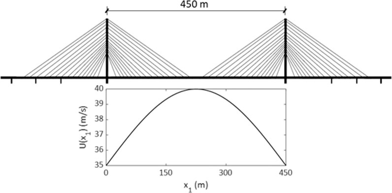
FIGURE 1. Spanwise fluctuating alongwind: for bridge deck: (A) illustrates the dimension of the main span of a bridge, and (B) shows the mean wind profile along the bridge deck.
The obtained samples of the one-dimensional horizontal wind field at a few selected points are illustrated in Figure 2. Figure 2A illustrates the time histories for selected points, where the mean wind velocity is included in the plot, showing that the time histories of the wind velocity near the middle of the main span of the bridge are associated with greater fluctuating winds than those near the pylons. The plot of the line wind field for selected times that are depicted in Figure 2B shows that the line wind field for a given time follows the assigned horizontal wind profile. Finally, the propagating line wind fields are shown in Figure 2C.
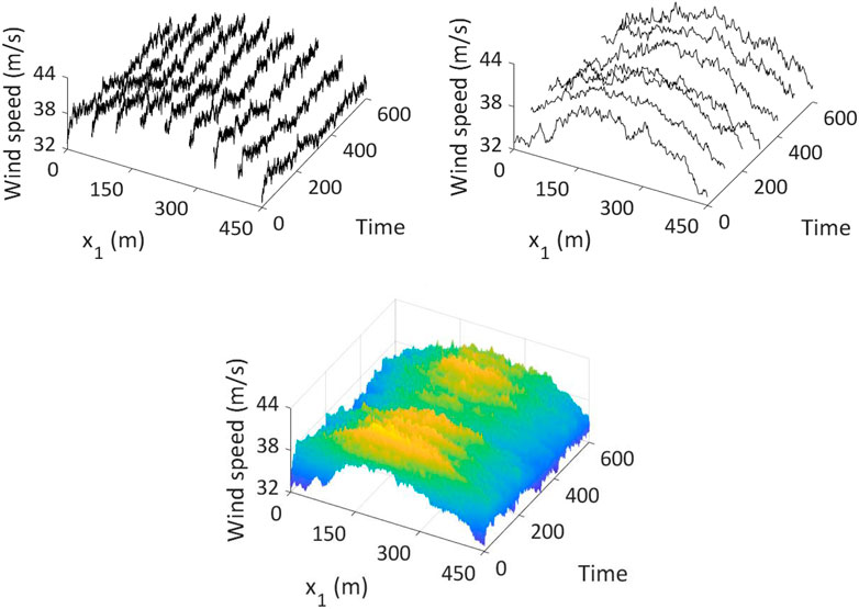
FIGURE 2. Typical simulated nonhomogeneous propagating wind field (the plots include the mean wind velocity): (A) shows simulated wind velocity plus the mean wind velocity at a few selected locations, (C) represents the wind velocity field at a few selected time, and (B) shows the propagating wind field along the bridge deck.
For assessing the adequacy of the simulated fluctuating wind, the simulation is run 25 times. The average PSD function of the simulated fluctuating wind velocities at three selected points along the bridge deck are evaluated and shown in Figure 3. The PSD functions calculated from the simulated samples compares well to the target PSD function at the considered sites.
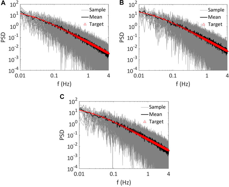
FIGURE 3. Comparison of the estimated power spectral density function (m2/s2) at three points along bridge deck by using 25 runs: (A) at the left pylon, (B) at 200 m from the left pylon and (C) at 400 m from the left pylon.
In addition to the above, the lagged coherence of the wind velocities for simulated records at three pairs of points is calculated. The evaluation of the lagged coherence is carried out in the τ-domain rather than the t-domain, so the calculated values are independent of time. A comparison of the calculated lagged coherence from the samples to the targets shown in Figure 4 indicates that the match is excellent for the target lagged coherence value greater than 0.4. For cases where the target lagged coherence is less than about 0.3, the lagged coherence from the simulated records is higher than that of the target value. This is expected since it is well-known that the lagged coherence even for the simulated white noise is in the order of about 0.2 (Bendat and Piersol, 1971).
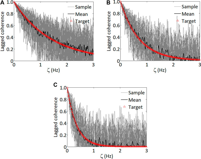
FIGURE 4. Variation of the lagged coherence for different separation by considering 25 simulation cycles: (A) Separation equal to 1.76 m, (B) Separation equal to 3.53 m, and (C) Separation equal to 7.06 m.
Example 2: This example is the same as the previous example except that the mean wind is considered to be equal to
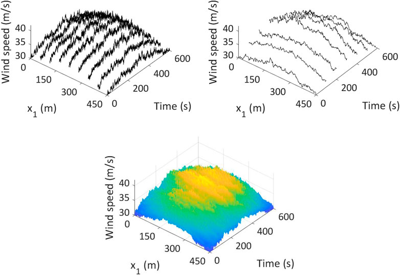
FIGURE 5. Simulated nonstationary and nonhomogeneous line wind field, including the mean wind velocity: (A) shows simulated wind velocity plus the mean wind velocity at a few selected locations, (C) represents the wind velocity field at a few selected time, and (B) shows the propagating wind field along the bridge deck.
Example 3. In this example, the two dimensional AM/FM and nonhomogeneous propagating wind fields are simulated for the area shown in Figure 6A. The bottom line of the area is 25 m above the ground surface, and the height of the area equals 30 m, and the width equals 450 m. The profile of the mean wind velocity is defined by,
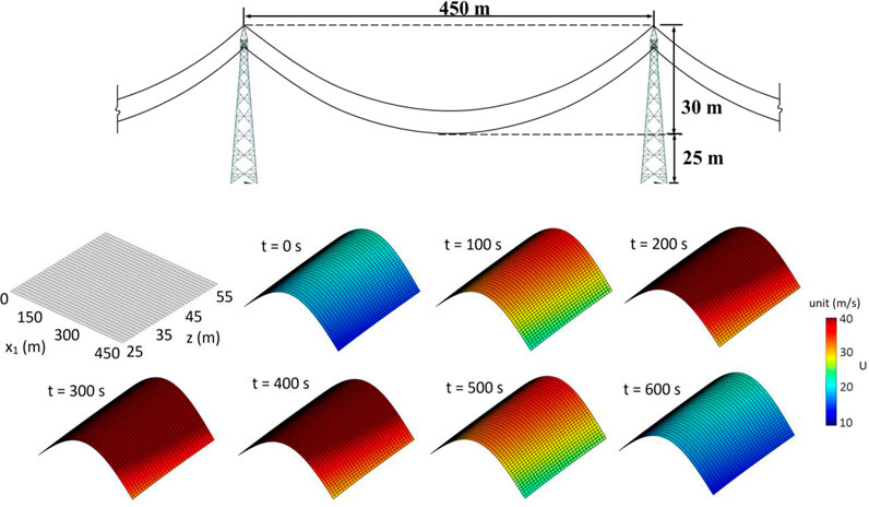
FIGURE 6. Definition for the simulation of two-dimensional wind fields: (A) shows the exposure area (not to scale), and (B) shows the mean wind profile in time and space.
which is shown in Figure 6B.
For the fluctuating winds, the FW-PSD shown in Eq. 27 is applicable with Cx1 = 20 and Cx2 = 16, zav =(25 + 30)/2 = 27.5 m and
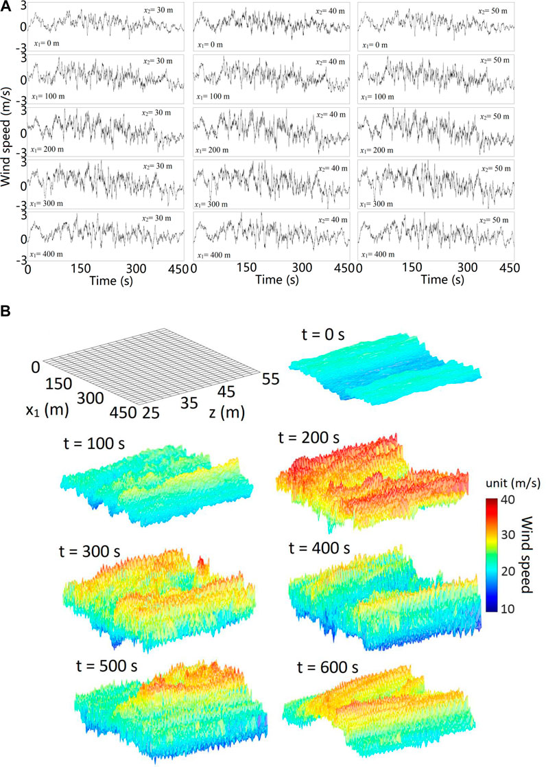
FIGURE 7. (A) Plots of samples of simulated time histories for the nonstationary and (B) nonhomogeneous wind field.
Conclusion
In the present study, a simple technique to simulate AM/FM and nonhomogeneous propagating wind fields is presented. The technique is based on the theoretical development indicating that the nonstationary wind velocity can be represented as amplitude modulated and frequency modulated stationary wind where the frequency modulation is achieved through the nonlinear time transformation.
Simple to use and implement equations to carry out the simulation for AM/FM one-dimensional line wind velocity field and two-dimensional wind velocity field are presented by incorporating the fast Fourier transform for computational efficiency. The use of the developed technique and its adequacy is illustrated through numerical examples.
Data Availability Statement
The original contributions presented in the study are included in the article/Supplementary Material, further inquiries can be directed to the corresponding author.
Author Contributions
All authors listed have made a substantial, direct, and intellectual contribution to the work and approved it for publication.
Funding
The financial support was received from the Natural Science and Engineering Research Council of Canada (RGPIN-2016-04814, for HP).
Conflict of Interest
The authors declare that the research was conducted in the absence of any commercial or financial relationships that could be construed as a potential conflict of interest.
Acknowledgments
We thank X.Z. Cui for his assistance in preparing the numerical examples.
References
Bendat, J. S., and Piersol, A. G. (1971). Random Data: Analysis and Measurement Procedures. New York: Wiley-Interscience.
Benowitz, B. A., and Deodatis, G. (2015). Simulation of Wind Velocities on Long Span Structures: A Novel Stochastic Wave Based Model. J. Wind Eng. Ind. Aerodynamics 147, 154–163. doi:10.1016/j.jweia.2015.10.004
Carassale, L., Solari, G., and Tubino, F. (2007). Proper Orthogonal Decomposition in Wind Engineering - Part 2: Theoretical Aspects and Some Applications. Wind and Structures 10 (2), 177–208. doi:10.12989/was.2007.10.2.177
Chay, M. T., Albermani, F., and Wilson, R. (2006). Numerical and Analytical Simulation of Downburst Wind Loads. Eng. Structures 28 (2), 240–254. doi:10.1016/j.engstruct.2005.07.007
Chen, J., Song, Y., Peng, Y., and Spanos, P. D. (2018). Simulation of Homogeneous Fluctuating Wind Field in Two Spatial Dimensions via a Joint Wave Number–Frequency Power Spectrum. J. Eng. Mech. 144 (11), 04018100. doi:10.1061/(asce)em.1943-7889.0001525
Chen, L., and Letchford, C. W. (2007). Numerical Simulation of Extreme Winds from Thunderstorm Downbursts. J. Wind Eng. Ind. Aerodynamics 95 (9), 977–990. doi:10.1016/j.jweia.2007.01.021
Chen, X., and Kareem, A. (2005). Proper Orthogonal Decomposition-Based Modeling, Analysis, and Simulation of Dynamic Wind Load Effects on Structures. J. Eng. Mech. 131 (4), 325–339. doi:10.1061/(asce)0733-9399(2005)131:4(325)
Davenport, A. G. (1967). Gust Loading Factors. J. Struct. Div. 93 (3), 11–34. doi:10.1061/jsdeag.0001692
Deodatis, G., and Shinozuka, M. (1989). Bounds on Response Variability of Stochastic Systems. J. Eng. Mech. 115 (11), 2543–2563. doi:10.1061/(asce)0733-9399(1989)115:11(2543)
Di Paola, M. (1998). Digital Simulation of Wind Field Velocity. J. Wind Eng. Ind. Aerodynamics 74-76, 91–109. doi:10.1016/s0167-6105(98)00008-7
Gradshteyn, I. S., and Ryzhik, I. M. (1994). Table of Integrals, Series and Products. 5th edn. New York: Academic.
Gurley, K., and Kareem, A. (1999). Applications of Wavelet Transforms in Earthquake, Wind and Ocean Engineering. Eng. structures 21 (2), 149–167.
Hong, H. P. (2004). Accumulation of Wind Induced Damage on Bilinear SDOF Systems. Wind and Structures 7 (3), 145–158. doi:10.12989/was.2004.7.3.145
Hong, H. P. (2016). Modeling of Nonstationary Winds and its Applications. J. Eng. Mech. 142 (4), 04016004. doi:10.1061/(asce)em.1943-7889.0001047
Hong, H. P., and Hong, H. P. (2007). Assessment of Ductility Demand and Reliability of Bilinear Single-Degree-of-Freedom Systems Under Earthquake Loading. Can. J. Civil Eng. 34 (12), 1606–1615.
Huang, G., and Chen, X. (2009). Wavelets-based Estimation of Multivariate Evolutionary Spectra and its Application to Nonstationary Downburst Winds. Eng. Structures 31 (4), 976–989. doi:10.1016/j.engstruct.2008.12.010
Irwin, P. A. (2009). Wind Engineering Challenges of the New Generation of Super-tall Buildings. J. Wind Eng. Ind. Aerodynamics 97 (7-8), 328–334. doi:10.1016/j.jweia.2009.05.001
King, J. P. C. (2003). The Foundation and the Future of Wind Engineering of Long Span Bridges—The Contributions of Alan Davenport. J. Wind Eng. Ind. Aerodynamics 91 (12-15), 1529–1546. doi:10.1016/j.jweia.2003.09.007
Krenk, S. (1996). Wind Field Coherence and Dynamic Wind Forces. Proc. IUTAM Symposium on Advances in Nonlinear Stochastic Mechanics. Dordrecht: Kluwer, 269–278. doi:10.1007/978-94-009-0321-0_25
Li, Y., and Kareem, A. (1991). Simulation of Multivariate Nonstationary Random Processes by FFT. J. Eng. Mech. 117 (5), 1037–1058. doi:10.1061/(asce)0733-9399(1991)117:5(1037)
Li, Y., Togbenou, K., Xiang, H., and Chen, N. (2017). Simulation of Non-stationary Wind Velocity Field on Bridges Based on Taylor Series. J. Wind Eng. Ind. Aerodynamics 169, 117–127. doi:10.1016/j.jweia.2017.07.005
Mann, J. (1994). The Spatial Structure of Neutral Atmospheric Surface-Layer Turbulence. J. Fluid Mech. 273, 141–168. doi:10.1017/s0022112094001886
Mantoglou, A., and Wilson, J. T. (1982). The Turning Bands Method for Simulation of Random Fields Using Line Generation by a Spectral Method. Water Res. Res. 18 (5), 1379–1394.
Momomura, Y., Marukawa, H., Okamura, T., Hongo, E., and Ohkuma, T. (1997). Full-scale Measurements of Wind-Induced Vibration of a Transmission Line System in a Mountainous Area. J. Wind Eng. Ind. Aerodynamics 72, 241–252. doi:10.1016/s0167-6105(97)00240-7
Peng, Y., Wang, S., and Li, J. (2018). Field Measurement and Investigation of Spatial Coherence for Near-Surface strong Winds in Southeast China. J. Wind Eng. Ind. Aerodynamics 172, 423–440. doi:10.1016/j.jweia.2017.11.012
Priestley, M. B. (1965). Power Spectral Analysis of Nonstationary Random Processes. J. Sound Vib. 6 (1), 86–97. doi:10.1016/0022-460X(67)90160-5
Samaras, E., Shinzuka, M., and Tsurui, A. (1985). ARMA Representation of Random Processes. J. Eng. Mech. 111 (3), 449–461. doi:10.1061/(asce)0733-9399(1985)111:3(449)
Shinozuka, M., and Deodatis, G. (1996). Simulation of Multi-Dimensional Gaussian Stochastic fields by Spectral Representation. Appl. Mech. Rev. 49 (1), 29–53. doi:10.1115/1.3101883
Shinozuka, M., and Jan, C.-M. (1972). Digital Simulation of Random Processes and its Applications. J. Sound Vibration 25 (1), 111–128. doi:10.1016/0022-460x(72)90600-1
Simiu, E., and Scanlan, R. H. (1996). Wind Effects on Structures – Fundamentals and Applications to Design. New York, NY: John Wiley & Sons.
Solari, G., Carassale, L., and Tubino, F. (2007). Proper Orthogonal Decomposition in Wind Engineering - Part 1: A State-Of-The-Art and Some Prospects. Wind and Structures 10 (2), 153–176. doi:10.12989/was.2007.10.2.153
Solari, G., and Piccardo, G. (2001). Probabilistic 3-D Turbulence Modeling for Gust Buffeting of Structures. Probabilistic Eng. Mech. 16 (1), 73–86. doi:10.1016/s0266-8920(00)00010-2
Song, Y., Chen, J., Peng, Y., Spanos, P. D., and Li, J. (2018). Simulation of Nonhomogeneous Fluctuating Wind Speed Field in Two-Spatial Dimensions via an Evolutionary Wavenumber-Frequency Joint Power Spectrum. J. Wind Eng. Ind. Aerodynamics 179, 250–259. doi:10.1016/j.jweia.2018.06.005
Spanos, P. D., and Zeldin, B. A. (1998). Monte Carlo Treatment of Random fields: a Broad Perspective. Appl. Mech. Rev. 51, 219–237. doi:10.1115/1.3098999
Vickery, B. J. (1970). Wind Action on Simple Yielding Structures. J. Engrg. Mech. Div. 96 (2), 107–120. doi:10.1061/jmcea3.0001221
Xu, Y. L., and Chen, J. (2004). Characterizing Nonstationary Wind Speed Using Empirical Mode Decomposition. J. Struct. Eng. 130 (6), 912–920. doi:10.1061/(asce)0733-9445(2004)130:6(912)
Yang, S. C., and Hong, H. P. (2016). Nonlinear Inelastic Responses of Transmission tower-line System under Downburst Wind. Eng. Structures 123, 490–500. doi:10.1016/j.engstruct.2016.05.047
Yang, S. C., Liu, T. J., and Hong, H. P. (2017). Reliability of tower and tower-line Systems under Spatiotemporally Varying Wind or Earthquake Loads. J. Struct. Eng. 143 (10), 04017137. doi:10.1061/(asce)st.1943-541x.0001835
Keywords: nonstationary, nonhomogeneous, wind field, spatially varying mean wind velocity, simulation
Citation: Hong P and Hong HP (2021) Simulation of Nonstationary and Nonhomogeneous Wind Velocity Field by Using Frequency–Wavenumber Spectrum. Front. Built Environ. 7:636815. doi: 10.3389/fbuil.2021.636815
Received: 02 December 2020; Accepted: 12 May 2021;
Published: 28 May 2021.
Edited by:
Weichiang Pang, Clemson University, United StatesCopyright © 2021 Hong and Hong. This is an open-access article distributed under the terms of the Creative Commons Attribution License (CC BY). The use, distribution or reproduction in other forums is permitted, provided the original author(s) and the copyright owner(s) are credited and that the original publication in this journal is cited, in accordance with accepted academic practice. No use, distribution or reproduction is permitted which does not comply with these terms.
*Correspondence: H. P. Hong, aG9uZ2hAZW5nLnV3by5jYQ==