 Mustafa K. Masood
 Antti Aikala
 Olli Seppänen
 Vishal Singh
94% of researchers rate our articles as excellent or good
Learn more about the work of our research integrity team to safeguard the quality of each article we publish.
Find out more
ORIGINAL RESEARCH article
Front. Built Environ. , 21 December 2020
Sec. Construction Management
Volume 6 - 2020 | https://doi.org/10.3389/fbuil.2020.581295
Automatic reality capture and monitoring of construction sites can reduce costs, accelerate timelines and improve quality in construction projects. Recently, automatic close-range capture of the state of large construction sites has become possible through crane and drone-mounted cameras, which results in sizeable, noisy, multi-building as-built point clouds. To infer construction progress from these point clouds, they must be aligned with the as-designed BIM model. Unlike the problem of aligning single buildings, the multi-building scenario is not well-studied. In this work, we address some unique issues that arise in the alignment of multi-building point clouds. Firstly, we show that a BIM-based 3D filter is a versatile tool that can be used at multiple stages of the alignment process. We use the building-pass filter to remove non-building noise and thus extract the buildings, delineate the boundaries of the building after the base is identified and as a post-processing step after the alignment is achieved. Secondly, in light of the sparseness of some buildings due to partial capture, we propose to use the best-captured building as a pivot to align the entire point cloud. We propose a fully automated three-step alignment process that leverages the simple geometry of the pivot building and aligns partial xy-projections, identifies the base using z-histograms and aligns the bounding boxes of partial yz-projections. Experimental results with crane camera point clouds of a large construction site show that our proposed techniques are fast and accurate, allowing us to estimate the current floor under construction from the aligned clouds and enabling potential slab state analysis. This work contributes a fully automated method of reality capture and monitoring of multi-building construction sites.
The need for automating progress monitoring in construction projects is well-established in light of the waste involved in manually inspecting sites and updating records (Golparvar-Fard et al., 2011). In the past decade, efforts toward automation have benefited from advancements in on-site spatial survey technologies, which provide as-built information in the form of 2D images and 3D point clouds (Yang et al., 2015b; Wang and Kim, 2019), as well as improvements in computer vision techniques for processing this data (Seo et al., 2015; Zhong et al., 2019). An effective method for extracting useful information from as-built point clouds is to align them with the as-designed BIM model (Bosché, 2010). This method has opened up a plethora of applications in construction, such as construction progress tracking, safety management and dimensional quality management (Wang and Kim, 2019).
In essence, the problem of aligning as-built and as-designed models is that of point cloud registration, a well-studied topic in Computer Vision (Pomerleau et al., 2015). When applied to the context of the built environment, point cloud registration becomes complex due to the many occlusions, self-similarities and non-model points, which make automation of this pipeline very challenging (Bueno et al., 2018). Several solutions have been proposed for achieving fast and accurate alignment in the construction context (Wang and Kim, 2019), but they need to be updated in the face of changing trends in reality capture of construction.
A recent development is the emergence of multi-building point clouds, made possible by the integration of crane or drone-mounted cameras and photogrammetric techniques. The multi-building scenario presents the problem of isolating the buildings from a noisy construction site point cloud to enable effective alignment with the as-designed Building Information Model (BIM). An initial coarse alignment can be achieved by converting the as-built point cloud into the coordinate system of the as-designed BIM. Further alignment can be achieved by studying point (Kim et al., 2013c) or plane correspondences (Bueno et al., 2018) between the point clouds to be registered, although the latter is more natural for the built environment. Finally, fine alignment can be achieved by the Iterative Closest Point (ICP) algorithm (Besl and McKay, 1992) and its variants (Yang et al., 2015a). For all these registration approaches, removal of outliers is necessary to ensure fast and accurate results. In the case of multi-building point clouds, the outlier ratio is especially large. An efficient method to remove non-building noise is therefore highly desirable.
Another issue that can arise with multi-building point clouds that do not have complete coverage of the entire site is a significant disparity in the quality of different buildings. Buildings that are only partially captured and therefore fragmented can be an obstacle to accurate registration. Also, once a building is extracted from the multi-building point cloud, its base must be identified to accurately delineate the profile of the building.
To address these issues, we present the following solutions. First, we propose a BIM-based 3D bounding box filter, which we call a building-pass filter, to remove non-building noise. The filter defines a region of interest based on the outer limits of the BIM model and applies an efficient kd-tree-based search for building points. Such a filter has been used before as a preprocessing step (Han et al., 2018), but we use it additionally as an interim step during alignment and as a postprocessing step. To address the disparity in data quality across buildings, we present an approach to define a pivot building from which we obtain the required transformation for the entire multi-building point cloud. We also present a strategy using z-histograms to identify the base of buildings and infer the floor number from the aligned as-built point cloud. We call this algorithm BEAM (BIM-based Extraction and Alignment for Multi-building Point Clouds). The performance of the algorithm is evaluated by comparing it with manually generated ground truth transformations and examining the proportion of the cast-in-place roof slab that can be correctly extracted after alignment.
Additionally, this is one of few works that study crane camera point clouds. In a previous study (Masood et al., 2019), we tested a building extraction strategy on crane camera point clouds that did not make use of the as-designed BIM, in light of some point clouds in our dataset that were not georeferenced and could thus not easily be aligned with the model. However, georeferencing as-built data based on site referencing systems is a common practice in the industry (Wang and Kim, 2019) and is thus considered necessary for this work. Crane camera technology offers some key advantages over its counterparts like Light Detection And Ranging (LiDAR) and Unmanned Aerial Vehicles (UAVs), such as being fully automated, low-cost, and low-labor (Tuttas et al., 2016). The 3D point clouds obtained from crane cameras can allow daily and automatic inference of the current floor under construction, while 2D images can be used to infer the state of cast-in-place concrete roof slabs.
This paper is organized as follows: section 2 discusses related work; section 3 describes the crane camera dataset; section 4 explains the BEAM algorithm; section 5 presents the results and discussion, including a potential application of mapping the output of BEAM to 2D crane camera images; section 6 discusses some limitations of this work; and section 7 presents the conclusions.
In this section, we study previous works on the following three central themes of our paper: (i) Crane camera point clouds; (ii) Fully automated alignment of as-built data with as-designed BIM data; and (iii) Building extraction in the presence of noise.
In a comprehensive review of point cloud data acquisition techniques, Wang et al. (2019) identified Light Detection And Ranging (LiDAR) and photogrammetry (including videogrammetry) as the main methods of acquiring point clouds for construction applications. Typically, 3D data in construction has been captured using LiDAR, which provides high-precision point clouds and has been the technology of choice in some important past works (Bosché, 2010; Kim et al., 2013b; Zhang and Arditi, 2013; Bosché et al., 2015). However, laser scanners are expensive and require expert labor, which makes them unsuitable for continuous progress monitoring (Rebolj et al., 2017). Large areas are surveyed using Airborne LiDAR, which involves the significant expense of a piloted airplane carrying specialist laser scanning equipment (Johnson et al., 2014). In addition, Airborne LiDAR produces a distant view of the site that is not suited for close-range analysis.
According to Wang et al. (2019), photogrammetry has gained the most popularity due to the ease of access to the required equipment and the maturity of software packages. Photogrammetric point clouds are obtained from photographic images. Some past works used fixed on-site cameras (Golparvar-Fard et al., 2011; Kim et al., 2013a; Omar et al., 2018) for image capture, but focused only on a small segment of the construction site. A large number of devices would be required to achieve complete coverage of the construction site, since each visible point needs to be covered by at least two cameras (Braun et al., 2015). Attaching cameras to UAVs is becoming popular (Ham et al., 2016) and results in high coverage of the construction site. But UAVs have certain disadvantages. Aside from the need for flight permissions (Cardot, 2017), there are restrictions such as a security distance to be maintained from buildings and cranes, and maximal flight heights, which can pose a problem for tall buildings (Tuttas et al., 2016). Also, UAVs can only operate in the active area of construction when the cranes do not move, such as during breaks. Additionally, the risk of collisions, image quality deterioration due to bad weather and the difficulties in camera pose estimation with the continuous position changes of the UAV are inhibiting factors (Bang et al., 2017).
Wang and Kim (2019) conducted a comprehensive review of the application of point cloud data in the construction industry. It is evident that crane camera point clouds have received little attention. We review the exceptions subsequently. Tuttas et al. (2016) were the first to study as-built point clouds generated from crane cameras. They did a comparative analysis of image acquisition from crane cameras with hand-held cameras and UAVs. Based on their experiments, the authors suggested that despite the effort required to mount the camera and limited flexibility due to the limited range of motion of cranes, crane cameras are the best technique in terms of automation, safety and effort required. Xu et al. (2018) presented a method to detect and reconstruct scaffolding components from point clouds. They proposed a 3D local feature descriptor to extract features that were used to train a machine learning classifier to identify points belonging to linear straight objects. Despite good results on noisy crane camera point clouds, the authors suggested that outlier removal prior to applying the descriptor could improve the performance.
Braun et al. (2015) presented a method to detect built elements in an as-built crane camera point cloud. They used two cameras mounted on the boom of a crane to acquire images. The authors proposed to establish the sequence of construction of elements in the form of a “precedence relationship” graph. This was meant to track the built status of occluded elements, which could be inferred from the graph since it could not from the point cloud. However, such element-wise analysis requires the registration of the point cloud with the BIM model, which they ensured by manually inserting control points. The registration is therefore not fully automatic. In the next section, we review key past works that deal with fully automated point cloud registration in the construction context.
Following the typical point cloud registration pipeline, as-built and as-designed point clouds can be aligned by preprocessing to remove noise, coarse registration to achieve a rough alignment and fine registration to achieve near-optimal alignment. Preprocessing is discussed in section 2.3. As for coarse registration, some important early works proposed plane-matching (Bosché, 2012) and Principal Component Analysis (PCA)-based alignment (Kim et al., 2013b), but a recent review paper identifies the work of Bueno et al. (2018) as the state-of-the-art in the construction context. The approach in this work is to find matching sets of plane patches (and not just planes as in Bosché, 2012) in the as-built and as-designed data, find a set of transformations between these patches and then shortlist the best transformation through a series of support-assessment stages. The plane-based registration framework presented in this work is a robust approach that fits naturally to the built environment and was shown to successfully register different kinds of buildings. However, in cases when the geometry of the building is simple, some assumptions can be made which obviate the need for extracting planes and assessing support. Instead of searching for matching planes in the entire point cloud and assessing a large set of transformations, we can simply align the 2D projections of the top and facade of the buildings. In Wang et al. (2016), the problem of 3D transformation was converted to the simpler 2D case by aligning 2D projections. We take a similar approach in this work, except that instead of obtaining the 2D projection from a fitted plane, we obtain it by directly projecting the as-built point cloud. Additionally, we project only part of the as-built point cloud to ensure that noise at the base does not interfere with the alignment. Also, aside from alignment, we require filtering of fine noise and base identification, which we achieve by strategic application of a BIM-based filter and z-histograms, respectively.
For fine registration, the ICP algorithm is the standard approach (Bosché, 2010; Kim et al., 2013b; Bueno et al., 2018). However, the ICP algorithm requires point matching, which involves the assessment of all as-built data points. This can create a significant computational overhead when dealing with multi-building point clouds that contain a large amount of noise. Bosché (2010) suggested that some form of point sampling should be used to reduce the computational cost of ICP. Our proposed BIM-based filter removes non-building points efficiently and thus removes the need for analyzing the entire as-built point cloud. A recent work presents a method to speed up ICP by removing ground points from laser-scanned data for robot navigation (Li et al., 2019). Aside from the different data-type and application, our work differs from ground point extraction in the sense that we need to remove all non-building points, regardless of their being ground or non-ground points. This requirement of ours can be classed as building extraction, which we review in the next section.
When as an as-designed model is not present, or the disparity between the as-designed and as-built data is large (such as in early phases of construction), as-built data separated temporally can be matched by finding feature correspondences across 2D images (Tuttas et al., 2017). However, we do not explore as-built vs as-built registration in this work.
The problem of building extraction is to identify and segment buildings from visual data of a scene. Building extraction techniques have largely been developed for distant aerial imagery for urban planning and monitoring applications (Tomljenovic et al., 2015; Boonpook et al., 2020). Building extraction can either be data-driven (Nguyen et al., 2020) or model-driven (Zheng and Weng, 2015). Data-driven methods are the natural choice when a suitable model is not present. A previous work of ours (Masood et al., 2019) proposed a building extraction strategy based on 3D convex hull volumes of clusters on an as-built point cloud, based on the observation that buildings are larger than non-building elements. This work did not depend either on the BIM model or the georeferencing of the point cloud to identify buildings. However, the algorithm could suffer in the early stages of construction when non-building elements may be more voluminous than the building area.
When a suitable model is present, model-driven building extraction is more robust (Li et al., 2020). For example, Karantzalos and Paragios (2008) proposed a set of building templates as shape priors to guide the segmentation of buildings from aerial imagery, achieving superior results to pure intensity-based segmentation. In the construction context, BIM models are now ubiquitous and can be naturally used as strong geometric and semantic priors for building extraction from multi-building construction scenes. For example, Han et al. (2018) used the minimum and maximum values of the BIM model to filter a large UAV point cloud, leading to an 80% reduction in the number of points. They included a threshold to account for registration errors. In this work, we build on the idea of BIM-based filtering by defining a 3D bounding box filter based on the BIM model. In addition to global filtering to extract buildings, we show how in combination with z-histograms of the building, such a BIM-based filter can aid in base identification and as a postprocessing step after alignment. A recent work (Huang et al., 2020) uses the 1D histogram of the horizontal projection of a building point cloud to reason in the frequency domain about vertical translation. We instead use the z-histogram to identify the base of the building based on the intuition that the base has a greater point count than the noisy regions.
The data was collected on the site of the Tripla project located in Helsinki, Finland, which includes a shopping center, hotel, housing and offices. The total area of the site is 183,000 floor m2. A crane camera solution developed by Pix4D was used to collect data (Cardot, 2017). Two independent cameras were mounted on the jib of a tower crane. The cameras were located approximately 13 and 37 m from the rotation axis of the crane, respectively and their viewing direction was toward the ground. The vertical height of the crane boom, and thus of the cameras, was about 100 m from sea level. Since the cameras were in nadir orientation, the viewing directions of the camera did not change when the crane moved. The focal length per detector width was approximately 28 mm for 35 mm film. Images were automatically taken as the crane would begin operation and then transferred to the Pix4D Cloud, where they were converted to 2D maps and 3D point clouds. Points were calculated with the stereo baseline across the crane jib and the overlap in the turning direction was at least 60%. The size of the images was 3648 × 5472 pixels. The entire process, from image capture to daily point cloud, was automatic. From a point cloud dataset spanning August to November 2018, eight point clouds were selected based on their being successfully georeferenced and also containing at least some segment of all three buildings on the site. The georeferencing was performed automatically using Global Positioning System (GPS) values. The dates, densities and point counts of the point clouds are shown in Table 1.
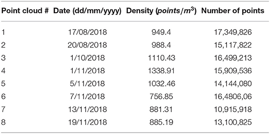
Table 1. Description of as-built point cloud dataset.
Figure 1A shows the as-designed BIM model of the buildings with their respective labels, while Figure 1B shows the corresponding labels on an as-built point cloud.
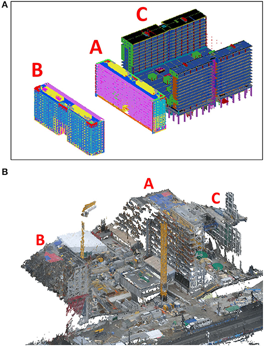
Figure 1. Construction site in Helsinki, Finland with the three buildings labeled A, B, and C in (A) an as-designed BIM model and (B) an as-built point cloud.
The point clouds are too fragmented for element-wise identification, but the geometry of the facade is retained to a reasonable degree. This can be used for estimating the number of the current floor under construction. The point cloud contains a large amount of non-building noise, which presents two problems: (i) it can interfere with the alignment with the BIM model and (ii) there would a large computational overhead for analyzing the entire point cloud. Also, the base contains multiple occlusions which can interfere with identifying the boundaries of the building. Additionally, while none of the buildings is fully captured, buildings B and C are relatively more fragmented.
In order to achieve good alignment, the non-building noise must be eliminated. Following this, the best-captured building can be used to obtain the necessary transformations for alignment. Then, the base of the buildings (which may be occluded) must be identified. Finally, the building point clouds must be aligned with the BIM model. Once this is achieved, the current floor under construction can be inferred from the aligned cloud. In the next section, we present our method of achieving these objectives in light of these requirements.
In this section, we present BEAM, which is our solution to address the problems outlined in section 3. An initial coarse alignment is achieved by conversion of the global coordinate system (in which the as-built point clouds are originally defined) to the local coordinate system (of the BIM model) followed by correction of the zero-point offset and angular offset, which we easily obtain from design information. To address the problem of non-building noise, we apply the building pass filter to remove the coarse non-building noise, leaving only some noise around the building profiles. Then, for further coarse alignment, fine noise removal and base detection, we select the best-captured building as the pivot building and apply the following steps. We align the xy projections (using ICP), apply the building-pass filter to remove some fine noise, identify the base of the buildings using z-histograms, align the yz projections using bounding box alignment and apply the building-pass filter again for further fine noise removal.We then apply the 2D transformations obtained for the pivot building to the other buildings, along with the same strategic application of the building-pass filter and base alignment. The result is a well-filtered and BIM-aligned as-built point cloud, from which we infer the current floor under construction. The algorithm is illustrated in Figure 2 and explained subsequently.

Figure 2. Flowchart showing major components of BEAM.
Let a construction site point cloud from the dataset (of eight point clouds) be with for i = 1, ..., N. Let be a point cloud obtained from the as-designed BIM model. Our target is to obtain , which is the set of point clouds corresponding to buildings A, B, and C, such that is aligned with . The first step is coordinate conversion which is explained below.
The location data in the as-built point clouds is in terms of global coordinates defined by the Universal Transvers Mercator (UTM) system for zone 35 V, also known as ETRS-TM35FIN (Uikkanen, n.d.). UTM coordinates consist of easting and northing values (E, N). The BIM model is defined in terms of local (X, Y, Z) coordinates. The axes of the local coordinate system are selected so as to follow nearby streets and outer-wall directions of buildings. The zero point for the BIM model is set to be in the South-West direction from the site area, thus giving positive X and Y coordinate values for all locations on the site. Let's refer to this zero point, expressed in UTM coordinates, as (E0, N0). The height value Z is the same for both local and global coordinates and it follows the N2000 coordinate system, which expresses the height from the theoretical sea level mean height. Local X and Y coordinate axes differ by θ = 11.4° from the global E and N axes, as is illustrated in Figure 3. Both the global zero point and angular offset were obtained at the start of the project (from the architect and site drawing, respectively), after which we were able to apply the conversion to all point clouds without any manual intervention.
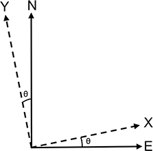
Figure 3. Angular deviation of X and Y axes of local coordinate system (of the BIM model) from the UTM35V global coordinate system (E, N).
In order to convert the point cloud into local coordinates, we shift the as-built point cloud by the local zero and rotate by θ, as is expressed in the following equation:
We will refer to the converted point cloud as . The results of conversion for Point Cloud 1 are shown in Figure 4. As can be seen from the figure, the conversion leads to a rough alignment of the point cloud with the BIM model.
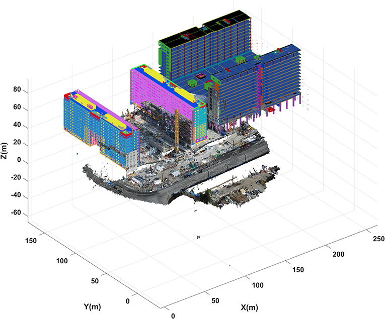
Figure 4. As-built Point Cloud 1 after coordinate conversion seen against the as-designed BIM model.
The building-pass filter is a 3D bounding box filter (Rusu and Cousins, 2011) whose parameters are defined using the BIM model to specify a region of interest that contains the buildings. The data points that fall within the region of interest are searched using a k-dtree, a modern formulation of which is given in Skrodzki (2019). We define the building-pass filter subsequently. Let the limits of be . The filter is a cuboid whose vertices are defined by as shown below:
We add a tolerance tol to bpf defined as follows:
The tolerance is required because the as-built point cloud is misaligned with the as-designed BIM to start with. Once the cuboidal region of interest is created, a 3D k-dtree is built to efficiently find the points in , which is explained subsequently. First, we determine the cutting dimension . This is the dimension in which two points pa and pb exist such that , where refers to the other two dimensions. After this, we sort the values in (held in a set S) and find the median of S. This median forms the root node of the tree. All values less than the median are assigned to the left child and those greater than the median to the right child. The algorithm then recurses on the children nodes. If the number of points corresponding to a particular node is less than the bucket size b (which we take as 5,000), we cease to partition the points and instead label the node as a leaf node. Note that we implement a leaf-based tree in which all the points are stored at the leaf nodes (and not at the inner nodes as in the case of non-leaf based trees). This considerably decreases the space required to store the tree (Behley et al., 2015). The computational complexity of building the kdtree is typically O(NlogN).
Once the kdtree is built, we can now efficiently search for points within the building-pass filter. The cutting threshold αnode, is defined as follows:
where node is the index of the current nodes in the kdtree and NS is the number of points in S. Equation (4) is the median of the elements of S when NS is even.If NS is odd, it is rounded to the nearest greater integer. Starting the tree traversal from the root node, if the maximum building-pass filter limits corresponding to the cutting dimension at the node exceed (or are equal to) αnode, we move to the right child of the current node. Then, if the minimum building-pass filter limits are less than (or equal to) αnode, we move to the left child of the current node. This continues until a leaf node is found. Now, the points in the leaf node are assessed for presence within the building-pass filter, after which the algorithm moves back up the tree to the next untested node. All leaf nodes that are of a lower index than the last visited leaf node cannot possibly contain the desired points and are thus eliminated from the search. For our dataset, for a bucket size of 5,000, the kdtree reduces the search space by 72% on average compared to a brute force search.
We apply the building-pass filter to with tol = 5 m to accommodate the initial misalignment. The results will be shown in section 5. With most of the non-building portion of removed, we achieve the set of unaligned building point clouds. To aid building-specific analysis, we define the corresponding set of as-designed point clouds obtained from the BIM model.
We select as the pivot building since it has the best coverage, find the required transformation for it and then apply the resulting transformations to and . Since the outer geometry of the building is simple, we can convert the 3D alignment to 2D by considering the 2D projections of the top and facade of the building. We first align the xy projections of the point clouds, after which we identify the base of the as-built point cloud, following which we align the yz projections of the point clouds. These steps are detailed subsequently.
We find the transformation Txy that aligns the xy projections of and using the standard point-to-point ICP algorithm. In order to prevent base noise from interfering with the alignment, we only project the top 50% of . We then apply Txy to to achieve an xy-aligned 3D as-built point cloud, to which we apply the building-pass filter to remove fine noise around the building profile. This time, we wish to filter only above the building and to its sides and wish to retain the base area for analysis in the next step. Thus, we set the minimum x and z-limits to −∞ and the maximum x-limit to ∞. All other limits remain as in Equation (2). Also, we can now set tol to zero since the point cloud is already xy-aligned. We denote the xy-aligned point cloud as .
Identifying the base of the building is a challenging task because of a concentration of construction noise at the base. Our strategy to identify the base is to study the histogram of the z-values at the base of the building and select the mode of these values, based on the intuition that the base of the building has a far greater point count than the noisy regions. We first take the yz projection of , downsample it with a grid filter and define the region of interest to be the bottom 20% portion of the building. We then construct the histogram with a bin width of 0.1 m and take the mode as the base height. For safety, we add a small tolerance of 0.1 m, which is effectively the histogram bin next to the mode bin. The histogram for Point Cloud 1 is shown in Figure 5. The peak corresponds to 31.9 m and thus 32 m is taken as the base height. Once the height is estimated, we can simply remove the points below base. The resulting point cloud is denoted as .
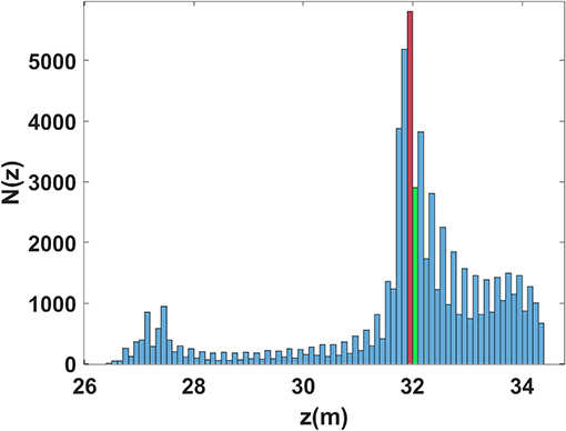
Figure 5. Histograms of z-values for the bottom 20% portion of building A for Point Cloud 1. The red bar corresponds to the mode bin and the green bar is the selected base height.
To perform the yz-alignment of and , we simply align their respective bounding boxes. However, if the y limits of the base extend beyond those of the overall y-limits of the building, the bounding box may become enlarged beyond the envelope of the building. In order to prevent this from distorting the y-alignment, we take the bounding box of the top 90% of the building. Then, we simply shift the bounding box by the difference between the bounding box edges which are normal to the y-axis. To perform z-alignment, we take the bounding box of the entire yz projection and shift it by the difference between the bounding box edges which are normal to the z-axis.
Once the yz-alignment is complete, we apply the building-pass filter again as defined in Equation (2) and with tol set to zero. Finally, we achieve the set of aligned building point clouds
In this section, we explain our strategy to estimate the current floor under construction. We first study the histogram of z-values between the ends of the yz projections of the building sections and select the largest z value (i.e., the largest height) as the height of the section. To ensure that our selected region of interest falls within the ends of the building section, we shrink the region of interest by 10% on each side. Also, to avoid selecting a z value corresponding to an outlier, we set a simple noise criterion as follows:
where ni is the number of points at the ith bin of the histogram, ntotal is the total number of points in the region of interest and γ is a noise threshold which we set to 0.005.
Once the height of each slab section is obtained, we use a rule base created from design heights to infer the floor number. Specifically, we check if the estimated floor height falls between the upper levels (according to the design) of the roof slabs of the previous and current floor. The rule base is shown in Table 2. We add a tolerance th of 1 m, considering that the floor height is 3.1 m. The results are presented in section 5.
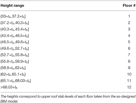
Table 2. Rule base used to infer floor number.
In this section, we discuss the results obtained by applying BEAM to our dataset of eight point clouds, following which we. To avoid congested illustrations, only point clouds 1 and 5 are illustrated.
Figure 6 illustrates the application of the building-pass filter to point clouds 1 and 5. The filter removes most of the non-building portion of the construction site. The misalignment is relatively less for Point Cloud 1 and thus the need for the tolerance may not be obvious. However, Point Cloud 5 is noticeably more misaligned, as is evident from the figure. Without a tolerance, the filter would remove some portion of the building. The filter leads to an average point count reduction of 63.32%.
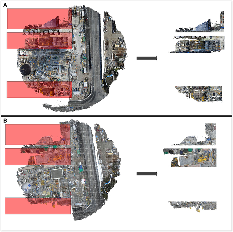
Figure 6. First application of the building-pass filter (with tolerance 5) to (A) Point Cloud 1 and (B) Point Cloud 5.
Figure 7 shows the xy-alignment for point clouds 1 and 5. The ICP algorithm corrects the angular orientation of both point clouds reasonably well. The results are similar for the entire dataset. Figure 8 shows the results for base detection for both point clouds. The base is identified correctly in both cases and the results are consistent across the entire dataset. Next, Figure 9 shows the yz-alignment for both point clouds. Point Cloud 5 is significantly misaligned in both y and z directions, but this is corrected effectively by the algorithm.
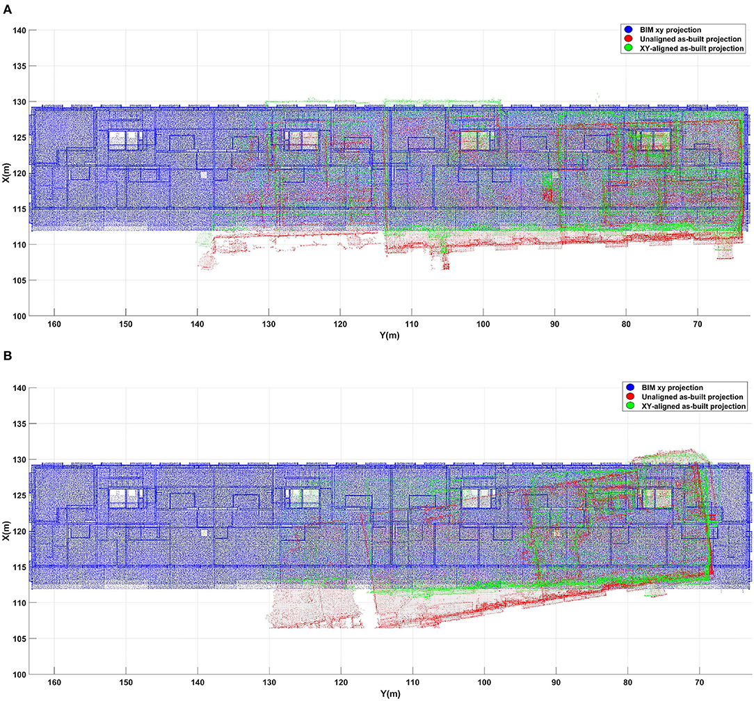
Figure 7. Alignment of xy projections using ICP for (A) Point Cloud 1 and (B) Point Cloud 5.
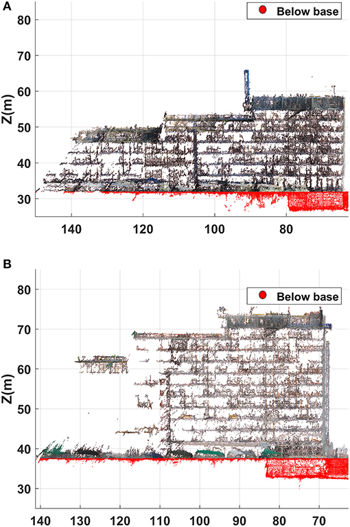
Figure 8. Base detection for (A) Point Cloud 1 and (B) Point Cloud 5.
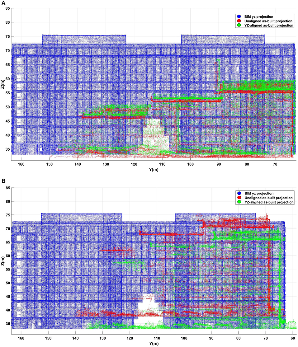
Figure 9. Alignment of yz projections for (A) Point Cloud 1 and (B) Point Cloud 5.
The following metrics were used to evaluate the registration accuracy and speed of the proposed algorithm:
• The difference between the transformations obtained from the proposed algorithm and the ground truth transformations, which were obtained by manually applying a rotation and translation to each aligned point cloud such that the cast-in-place slab of section 1 (see Figure 10) was finely aligned with the corresponding slab in the BIM model. The rotation (angular correction) was applied such that the slabs boundaries became parallel as judged by visual inspection. Then, translation was applied such that the bottom-right corners of the slabs (when viewed overhead) coincided. We report the angular and translation errors δR and δT, respectively, as defined below:
where T = [tx, ty, 0]. The accuracy of z-alignment is assessed in terms of the floor estimation, as discussed in section 4.
• Root-Mean-Square Error (RMSE), which is the Euclidean distance (in meters) between the aligned point clouds.
• Computation time (in seconds) to run BEAM on an Intel Core i7-9750HF CPU with 16 GB RAM in MATLAB-R2020a software.
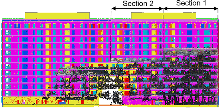
Figure 10. Description of building sections considered for floor estimation. The BIM model is shown in the backdrop.
The results are shown in Table 3. The mean angular error is 1.34 degrees, translation error is 2.6 m and RMSE is 0.7 m. These errors are small enough to enable further analysis of the slab states, as will be discussed in section 5.5. Considering the large average number of points in our dataset (14,940,000), the mean computation time of 159.86 s is small.
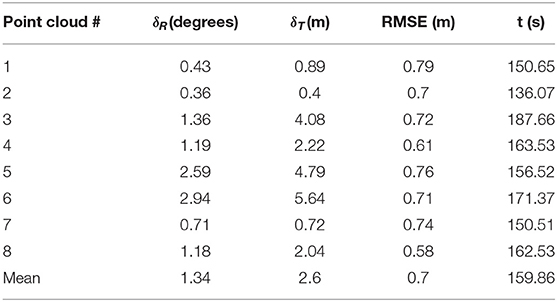
Table 3. Rotation error (δR), translation error (δT), RMSE, and computation time of BEAM.
The floor estimation was limited to building A, because only this building is consistently captured across its entire width. But since this building is not captured across its entire length, the floor level could be calculated for two out of four sections of the building, as is illustrated in Figure 10.
The ground truth of the current floor under construction was obtained from the Pix4D cloud by manual inspection. The results of the floor estimation are shown in Table 4. The current floor is estimated accurately for every point cloud, except for point cloud 4, where the actual floors “12” and “11” are estimated as “11” and “9,” respectively. As shown in Table 5, the estimated heights for sections 1 and 2 corresponding to Point Cloud 4 are 67.9 and 62.8 m, respectively, while floor 12 is detected beyond 69.03 m and floor 11 beyond 63 m. The reason for the misestimation is the small difference in scale between the BIM point cloud and the as-built point cloud, the latter being smaller.
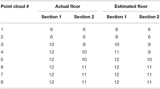
Table 4. Floor estimation results.
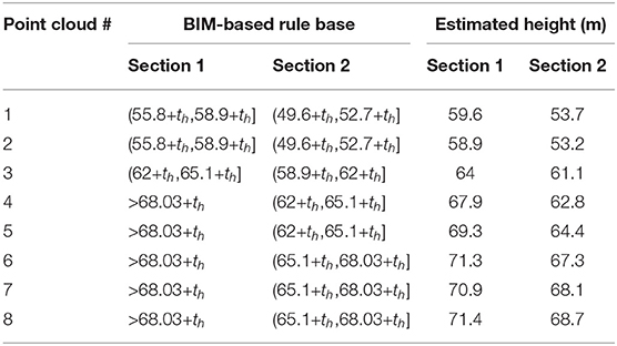
Table 5. Estimated slab heights shown against the rule base created from design heights.
Crane camera data could be used to enable remote monitoring of construction sites and automatic alerts in construction workflow when progress falls behind expectations, especially to aid those construction managers who are off-site and whose workflows require real-time knowledge of any deviations of plans. For example, automatic inference of the current floor under construction from BIM-aligned point clouds, as was demonstrated in this work, could keep managers informed of deviations from the schedule.
Another potential application is that once the current floor under construction is known, cast-in-place concrete roof slabs can be extracted. As we shall demonstrate subsequently, the slabs can be accurately extracted from the aligned as-built point cloud. We can measure the overlap between the slabs in the BIM model and those in the as-built point cloud using Intersection Over Union (Iou) (Csurka et al., 2013). For a reference area R and estimated area E, the IoU can be defined as:
To obtain the estimated slab areas, we manually determined the slab corners of sections 1 and 2 (see Figure 10) from the set of aligned clouds The reference slab areas were obtained from the BIM model. An average IoU of 0.833 was obtained. This is a good overlap that can be leveraged to infer the state of the slab. For example, Bang and Kim (2020) considered bounding boxes with IoU more than 0.80 to represent the same construction scene, therefore such bounding boxes were merged together before object recognition was performed.
Once the slab region is identified, we can map the 3D points to the corresponding 2D crane camera images used to create them. From these 2D images, we can infer whether the slab contains no formwork, formwork only, formwork and rebar or completed rebar, as shown in Figure 11.
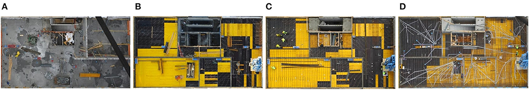
Figure 11. Different states of the slab: (A) No formwork, (B) Formwork, (C) Rebar, and (D) Rebar complete.
A generalized version of this application was explored by Dimitrov and Golparvar-Fard (Dimitrov and Golparvar-Fard, 2014), who used a bag-of-words model with a Support Vector Machine (SVM) for material recognition from site images. The authors considered 20 classes of materials. To improve the accuracy, they suggested that classes be limited to the material expected in a particular region under construction. Also, the authors suggested the need for identifying a region in a photograph belonging to a single material so that material classification could be restricted to that region. They suggested that these regions could be derived by back-projecting BIM element surfaces or points of a segmented point cloud onto site images. This kind of automated region extraction was explored in Aikala et al. (2019). In future work, we intend to automatically infer the slab state by formulating this as a scene recognition problem.
Due to incomplete coverage of the construction site by the cameras, the point clouds were fragmented. The most complete portion of the point cloud showed half of the facade of a building albeit a good view of the roof slabs. The rear was completely missing since it was not within the camera's field of view. Only a small segment of other buildings was available, which precluded them from floor estimation. Future work should consider how more crane cameras can be placed to extend coverage and examine a possible integration with drone images or images from fixed cameras.
In our data, and in fact for most buildings, the yz alignment is a case of matching straight edges, which is achieved by matching their bounding boxes. If the shapes are irregular, aligning the bounding boxes may not lead to a close alignment. In such cases, edge detection methods such as Sobel (Kittler, 1983) and Canny (Canny, 1986) or their modern variants such as CannySR (Akinlar and Chome, 2015), Predictive Edge Linking (Akinlar and Chome, 2016) and HT-Canny (Song et al., 2017) may be employed to trace the edges and then attempt the alignment.
The as-built point cloud was slightly out of scale with respect to the BIM model, which affected the accuracy of floor estimation. Automatically equalizing the scale of the as-built point cloud and BIM model should be addressed in future work.
Reality capture technologies are improving in level of automation and coverage, which is making it possible to acquire images and 3D point clouds of large, multi-building construction sites. In this work, we proposed BEAM, which is an algorithm that addresses some unique computational challenges that arise in the processing of multi-building point clouds. Firstly, to eliminate coarse and fine non-building noise, we presented a BIM-based building-pass filter. Results with eight point clouds of a three-building construction site showed that the filter offers a robust, flexible, and efficient way to remove both coarse and fine noise, leading to an average point count reduction of 63.32% for our dataset. Additionally, the building-pass filter can easily be applied to multi-building point clouds from other reality capture technologies (such as drones) and is relevant for point clouds of diverse densities. Secondly, in view of the holes in the data and disparity in data quality across buildings, we proposed an alignment strategy in which the best-captured building is selected as the pivot and partial 2D projections of the building are aligned. The registration accuracy was shown to agree well with ground truth, but could be further improved with fine alignment algorithms. We studied how the achieved alignment could facilitate slab analysis by calculating the slab region that could be extracted based on design dimensions. We achieved a mean IoU of 0.83, which we expect is a sufficiently good overlap for slab state analysis. Thirdly, we proposed a base identification strategy using z-histograms that is iteration-independent and could effectively identify the base for the entire dataset despite occlusions. As a result of successful alignment and base identification, floor numbers could be accurately calculated by mapping the height of the aligned cloud with design heights extracted from the BIM model. One floor was misestimated as a result of the small difference in scale between the as-built point cloud and the BIM model. This should be addressed by automatic scale-matching in future work.
The results of this study contribute to real-time construction progress monitoring by offering a fully automated, computationally feasible and accurate method of aligning daily construction site point clouds with as-designed models. This could facilitate remote management of construction sites, better organization of support functions such as procurement and logistics, and more accurate reporting of project status at the company or business unit level. Also, this is one of few works that uses crane camera data, which is an emergent technology that offers many benefits in terms of cost and automation compared with other reality capture techniques.
In future work, we intend to explore automatic recognition of the state of cast-in-place slabs by formulating it as a scene recognition problem that can be solved using a Bag-of-Words approach. Also, we intend to address the issues with data quality by installing fixed cameras on the crane and possibly augmenting them with drone data.
The datasets presented in this article are not readily available because the data belongs to a construction company. Requests to access the datasets should be directed to Mustafa K. Masood, bXVzdGFmYS4xLmtoYWxpZG1hc29vZEBhYWx0by5maQ==.
MM participated in data collection, designed the experiments, developed the methods, analyzed the results, and wrote the manuscript. AA participated in data collection, developed the coordinate conversion method, and contributed ideas to the other methods and gave critical feedback. OS specified requirements and gave critical feedback. VS gave critical feedback. All authors helped shape the research, analysis, and manuscript.
The authors declare that the research was conducted in the absence of any commercial or financial relationships that could be construed as a potential conflict of interest.
We thank YIT for providing the data for this study. The work was supported by the Reality Capture and Digitalizing Construction Workflows research projects funded by Business Finland, Aalto University and a consortium of companies. The work was partially supported by the Profi3 research programme on Digital technology ecosystems by Academy of Finland.
Aikala, A., Khalid, M., Seppänen, O., and Singh, V. (2019). Crane camera image preparation for automated monitoring of formwork and rebar progress. In Proceedings of the 36th CIB W78 Conference.
Akinlar, C., and Chome, E. (2015). “CannySR: using smart routing of edge drawing to convert canny binary edge maps to edge segments,” in 2015 International Symposium on Innovations in Intelligent SysTems and Applications (INISTA) (Madrid: IEEE). doi: 10.1109/INISTA.2015.7276784
Akinlar, C., and Chome, E. (2016). PEL: a predictive edge linking algorithm. J. Vis. Commun. Image Represent. 36, 159–171. doi: 10.1016/j.jvcir.2016.01.017
Bang, S., and Kim, H. (2020). Context-based information generation for managing UAV-acquired data using image captioning. Automat. Construct. 112:103116. doi: 10.1016/j.autcon.2020.103116
Bang, S., Kim, H., and Kim, H. (2017). UAV-based automatic generation of high-resolution panorama at a construction site with a focus on preprocessing for image stitching. Automat. Construct. 84, 70–80. doi: 10.1016/j.autcon.2017.08.031
Behley, J., Steinhage, V., and Cremers, A. B. (2015). “Efficient radius neighbor search in three-dimensional point clouds,” in 2015 IEEE International Conference on Robotics and Automation (ICRA) (Seattle, WA: IEEE). doi: 10.1109/ICRA.2015.7139702
Besl, P., and McKay, N. (1992). A method for registration of 3-d shapes. IEEE Trans. Pattern Anal. Mach. Infell. 14, 239–256. doi: 10.1109/34.121791
Boonpook, W., Tan, Y., and Xu, B. (2020). Deep learning-based multi feature semantic segmentation in building extraction from images of UAV photogrammetry. Int. J. Remote Sens. 42, 1–19. doi: 10.1080/01431161.2020.1788742
Bosché, F. (2010). Automated recognition of 3d CAD model objects in laser scans and calculation of as-built dimensions for dimensional compliance control in construction. Adv. Eng. Inform. 24, 107–118. doi: 10.1016/j.aei.2009.08.006
Bosché, F. (2012). Plane-based registration of construction laser scans with 3D/4D building models. Adv. Eng. Inform. 26, 90–102. doi: 10.1016/j.aei.2011.08.009
Bosché, F., Ahmed, M., Turkan, Y., Haas, C. T., and Haas, R. (2015). The value of integrating scan-to-BIM and scan-vs-BIM techniques for construction monitoring using laser scanning and BIM: the case of cylindrical MEP components. Automat. Construct. 49, 201–213. doi: 10.1016/j.autcon.2014.05.014
Braun, A., Tuttas, S., Borrmann, A., and Stilla, U. (2015). “Automated progress monitoring based on photogrammetric point clouds and precedence relationship graphs,” in Proceedings of the 32nd International Symposium on Automation and Robotics in Construction and Mining (ISARC 2015) (Oulu: International Association for Automation and Robotics in Construction). doi: 10.22260/ISARC2015/0034
Bueno, M., Bosché, F., González-Jorge, H., Martínez-Sánchez, J., and Arias, P. (2018). 4-plane congruent sets for automatic registration of As-Is 3d point clouds with 3D BIM models. Automat. Construct. 89, 120–134. doi: 10.1016/j.autcon.2018.01.014
Canny, J. (1986). A computational approach to edge detection. IEEE Trans. Pattern Anal. Mach. Intell. 6, 679–698. doi: 10.1109/TPAMI.1986.4767851
Cardot, S. (2017). Crane Camera Site Surveying. GIM Int. 31, 31–33. Available online at: https://www.gim-international.com/content/article/crane-camera-site-surveying
Csurka, G., Larlus, D., Perronnin, F., and Meylan, F. (2013). “What is a good evaluation measure for semantic segmentation?” in BMVC, 2013. (Bristol).
Dimitrov, A., and Golparvar-Fard, M. (2014). Vision-based material recognition for automated monitoring of construction progress and generating building information modeling from unordered site image collections. Adv. Eng. Inform. 28, 37–49. doi: 10.1016/j.aei.2013.11.002
Golparvar-Fard, M., Bohn, J., Teizer, J., Savarese, S., and Peña-Mora, F. (2011). Evaluation of image-based modeling and laser scanning accuracy for emerging automated performance monitoring techniques. Automat. Construct. 20, 1143–1155. doi: 10.1016/j.autcon.2011.04.016
Ham, Y., Han, K. K., Lin, J. J., and Golparvar-Fard, M. (2016). Visual monitoring of civil infrastructure systems via camera-equipped unmanned aerial vehicles (UAVs): a review of related works. Visual. Eng. 4:1. doi: 10.1186/s40327-015-0029-z
Han, K., Degol, J., and Golparvar-Fard, M. (2018). Geometry- and appearance-based reasoning of construction progress monitoring. J. Construct. Eng. Manage. 144:04017110. doi: 10.1061/(asce)co.1943-7862.0001428
Huang, R., Xu, Y., Hoegner, L., and Stilla, U. (2020). Temporal comparison of construction sites using photogrammetric point cloud sequences and robust phase correlation. Automat. Construct. 117:103247. doi: 10.1016/j.autcon.2020.103247
Johnson, K., Nissen, E., Saripalli, S., Arrowsmith, J. R., McGarey, P., Scharer, K., et al. (2014). Rapid mapping of ultrafine fault zone topography with structure from motion. Geosphere 10, 969–986. doi: 10.1130/GES01017.1
Karantzalos, K., and Paragios, N. (2008). Automatic model-based building detection from single panchromatic high resolution images. ISPRS Arch 37, 127–132.
Kim, C., Kim, B., and Kim, H. (2013a). 4d CAD model updating using image processing-based construction progress monitoring. Automat. Construct. 35, 44–52. doi: 10.1016/j.autcon.2013.03.005
Kim, C., Son, H., and Kim, C. (2013b). Automated construction progress measurement using a 4d building information model and 3d data. Automat. Construct. 31, 75–82. doi: 10.1016/j.autcon.2012.11.041
Kim, C., Son, H., and Kim, C. (2013c). Fully automated registration of 3d data to a 3d CAD model for project progress monitoring. Automat. Construct. 35, 587–594. doi: 10.1016/j.autcon.2013.01.005
Kittler, J. (1983). On the accuracy of the sobel edge detector. Image Vis. Comput. 1, 37–42. doi: 10.1016/0262-8856(83)90006-9
Li, P., Wang, R., Wang, Y., and Tao, W. (2020). Evaluation of the ICP algorithm in 3d point cloud registration. IEEE Access 8, 68030–68048. doi: 10.1109/ACCESS.2020.2986470
Li, X., Du, S., Li, G., and Li, H. (2019). Integrate point-cloud segmentation with 3d LiDAR scan-matching for mobile robot localization and mapping. Sensors 20:237. doi: 10.3390/s20010237
Masood, M., Pushkar, A., Seppänen, O., Singh, V., and Aikala, A. (2019). “Vbuilt: Volume-based automatic building extraction for as-built point clouds,” in ISARC. Proceedings of the International Symposium on Automation and Robotics in Construction (Banff, AB: IAARC Publications), 1202–1209. doi: 10.22260/ISARC2019/0161
Nguyen, T. H., Daniel, S., Gueriot, D., Sintes, C., and Le Caillec, J. M. (2020). Super-resolution-based snake model-an unsupervised method for large-scale building extraction using airborne LiDAR data and optical image. Remote Sens. 12:1702. doi: 10.3390/rs12111702
Omar, H., Mahdjoubi, L., and Kheder, G. (2018). Towards an automated photogrammetry-based approach for monitoring and controlling construction site activities. Comput. Indus. 98, 172–182. doi: 10.1016/j.compind.2018.03.012
Pomerleau, F., Colas, F., and Siegwart, R. (2015). A review of point cloud registration algorithms for mobile robotics. Found. Trends Robot. 4, 1–104. doi: 10.1561/9781680830255
Rebolj, D., Pučko, Z., Babič, N. Č., Bizjak, M., and Mongus, D. (2017). Point cloud quality requirements for scan-vs-BIM based automated construction progress monitoring. Automat. Construct. 84, 323–334. doi: 10.1016/j.autcon.2017.09.021
Rusu, R. B., and Cousins, S. (2011). “3d is here: point cloud library (PCL),” in 2011 IEEE International Conference on Robotics and Automation (Shanghai), 1–4. doi: 10.1109/ICRA.2011.5980567
Seo, J., Han, S., Lee, S., and Kim, H. (2015). Computer vision techniques for construction safety and health monitoring. Adv. Eng. Inform. 29, 239–251. doi: 10.1016/j.aei.2015.02.001
Skrodzki, M. (2019). Neighborhood data structures, manifold properties, and processing of point set surfaces (Ph.D. thesis). Freie Universität, Berlin, Germany.
Song, R., Zhang, Z., and Liu, H. (2017). Edge connection based canny edge detection algorithm. Pattern Recogn. Image Anal. 27, 740–747. doi: 10.1134/S1054661817040162
Tomljenovic, I., Häfle, B., Tiede, D., and Blaschke, T. (2015). Building extraction from airborne laser scanning data: an analysis of the state of the art. Remote Sens. 7, 3826–3862. doi: 10.3390/rs70403826
Tuttas, S., Braun, A., Borrmann, A., and Stilla, U. (2016). Evaluation of acquisition strategies for image-based construction site monitoring. ISPRS Int. Arch. Photogramm. Remote Sens. Spatial Inform. Sci. 41, 733–740. doi: 10.5194/isprs-archives-XLI-B5-733-2016
Tuttas, S., Braun, A., Borrmann, A., and Stilla, U. (2017). Acquisition and consecutive registration of photogrammetric point clouds for construction progress monitoring using a 4d BIM. PFG J. Photogramm.Remote Sens. Geoinformat. Sci. 85, 3–15. doi: 10.1007/s41064-016-0002-z
Uikkanen, E. (n.d.). Finnish Horizontal Coordinate Systems. Available online at: http://www.kolumbus.fi/eino.uikkanen/geodocsgb/ficoords.htm (accessed October 31, 2019).
Wang, Q., and Kim, M.-K. (2019). Applications of 3d point cloud data in the construction industry: a fifteen-year review from 2004 to 2018. Adv. Eng. Inform. 39, 306–319. doi: 10.1016/j.aei.2019.02.007
Wang, Q., Kim, M.-K., Cheng, J. C., and Sohn, H. (2016). Automated quality assessment of precast concrete elements with geometry irregularities using terrestrial laser scanning. Automat. Construct. 68, 170–182. doi: 10.1016/j.autcon.2016.03.014
Wang, Q., Tan, Y., and Mei, Z. (2019). Computational methods of acquisition and processing of 3d point cloud data for construction applications. Arch. Comput. Methods Eng. 27, 479–499. doi: 10.1007/s11831-019-09320-4
Xu, Y., Tuttas, S., Hoegner, L., and Stilla, U. (2018). Reconstruction of scaffolds from a photogrammetric point cloud of construction sites using a novel 3d local feature descriptor. Automat. Construct. 85, 76–95. doi: 10.1016/j.autcon.2017.09.014
Yang, J., Li, H., Campbell, D., and Jia, Y. (2015a). GO-ICP: a globally optimal solution to 3D ICP point-set registration. IEEE Trans. Pattern Anal. Mach. Intell. 38, 2241–2254. doi: 10.1109/TPAMI.2015.2513405
Yang, J., Park, M.-W., Vela, P. A., and Golparvar-Fard, M. (2015b). Construction performance monitoring via still images, time-lapse photos, and video streams: now, tomorrow, and the future. Adv. Eng. Inform. 29, 211–224. doi: 10.1016/j.aei.2015.01.011
Zhang, C., and Arditi, D. (2013). Automated progress control using laser scanning technology. Automat. Construct. 36, 108–116. doi: 10.1016/j.autcon.2013.08.012
Zheng, Y., and Weng, Q. (2015). Model-driven reconstruction of 3-d buildings using LiDAR data. IEEE Geosci. Remote Sens. Lett. 12, 1541–1545. doi: 10.1109/lgrs.2015.2412535
Keywords: reality capture, multi-building point cloud, building extraction, BIM model, construction site, crane cameras
Citation: Masood MK, Aikala A, Seppänen O and Singh V (2020) Multi-Building Extraction and Alignment for As-Built Point Clouds: A Case Study With Crane Cameras. Front. Built Environ. 6:581295. doi: 10.3389/fbuil.2020.581295
Received: 08 July 2020; Accepted: 24 November 2020;
Published: 21 December 2020.
Edited by:
Kevin Han, North Carolina State University, United StatesReviewed by:
Qian Wang, National University of Singapore, SingaporeCopyright © 2020 Masood, Aikala, Seppänen and Singh. This is an open-access article distributed under the terms of the Creative Commons Attribution License (CC BY). The use, distribution or reproduction in other forums is permitted, provided the original author(s) and the copyright owner(s) are credited and that the original publication in this journal is cited, in accordance with accepted academic practice. No use, distribution or reproduction is permitted which does not comply with these terms.
*Correspondence: Mustafa K. Masood, bXVzdGFmYS4xLmtoYWxpZG1hc29vZEBhYWx0by5maQ==
Disclaimer: All claims expressed in this article are solely those of the authors and do not necessarily represent those of their affiliated organizations, or those of the publisher, the editors and the reviewers. Any product that may be evaluated in this article or claim that may be made by its manufacturer is not guaranteed or endorsed by the publisher.
Research integrity at Frontiers
Learn more about the work of our research integrity team to safeguard the quality of each article we publish.