 Moniruzzaman Moni
 Youchan Hwang
 Oh-Sung Kwon
 Ho-Kyung Kim
 Un Yong Jeong
- 1Civil and Mineral Engineering, University of Toronto, Toronto, ON, Canada
- 2Department of Civil and Environmental Engineering, Seoul National University, Seoul, South Korea
- 3Gradient Wind Engineering Inc., Ottawa, ON, Canada
The wind tunnel test is one of the most reliable methods for evaluating the dynamic response of high-rise buildings considering wind-structure interaction. In conventional aeroelastic wind tunnel tests, the calibration of stiffnesses, masses and the damping properties of a scaled specimen is required. This takes extensive time and effort, especially when the tests need to be repeated with various geometric designs during design iterations. This study introduces a new testing method that combines a numerical simulation and the conventional aeroelastic wind tunnel test through the real-time hybrid simulation method. The stiffness, damping and partial mass of a scaled building model are represented numerically, while the rest of the mass, the wind-induced pressure around the model and the wind-structure interaction are represented physically in a wind tunnel. The building model in the wind tunnel rests on a base-pivoting system, which is controlled with a linear motor. The base moment induced by wind pressure and the inertial force from the mass of the physical specimen is measured; those measurements are then fed back into a numerical integration scheme. A delay-compensation scheme is implemented to minimize the effects of actuator delay on the dynamic response of the system. Several tests are carried out to validate and calibrate the developed test apparatus and control scheme including (1) tests for the identification of actuator delay, (2) free vibration tests for characterization of the dynamic properties of the hardware and the control system, and (3) wind tunnel tests for system validation through aeroelastic real-time hybrid simulation. This paper presents the overall design of the experimental apparatus, the adopted delay compensation and numerical integration schemes, and a summary of the test results. Test results confirmed that the developed experimental technique can replace the conventional aeroelastic wind tunnel tests of a building model, thus improving the efficiency of the aeroelastic wind tunnel testing.
Introduction
The number of new high-rise building construction has rapidly increased due to advancements in construction technology and to house the increasing populations in urban areas. For the design of these structures, proper estimation of lateral loads, such as earthquake and wind, is essential. Advancements in the seismic design of high-rise buildings have decreased their weight significantly to reduce the effect of earthquake forces on the buildings. If the weight of a high-rise structure decreases, the damping of the structure tends also to decrease, which in turn increases the vibration-induced acceleration of a structure subjected to wind load (Kanda et al., 2003). It is imperative to properly evaluate the dynamic response of high-rise buildings subjected to wind load at the design phase.
Both static and dynamic analysis methods have been used to evaluate the response of high-rise structures under wind loads. In the static analysis method, it is assumed that the dynamic interaction between a building and the wind load is negligible. In practice, static analysis is usually recommended for buildings up to 50 meters in height. This method cannot be applied to buildings that are tall, have a high slenderness ratio, or are susceptible to vibration under wind loads. For buildings with an aspect ratio (height to width ratio) of more than five and having the first natural period larger than 1 s, a dynamic analysis is required (Mendis et al., 2007). The dynamic effect of wind loads on tall buildings can be evaluated by performing computational fluid dynamics (CFD) analysis or boundary layer wind tunnel (BLWT) tests. Elshaer et al. (2015) used the CFD models, or surrogate models such as neural networks (NN), to evaluate the vibration of a tall building under wind load. The CFD analysis can accurately predict structural responses only for idealized boundary conditions at the expense of large computational time. However, CFD analysis cannot reliably simulate the wind fluctuation characteristics of natural winds and requires many assumptions and approximations. In such situations, the response of high-rise buildings subjected to wind can be more accurately evaluated with BLWT tests.
There are two test methods with a BLWT: the aerodynamic test method and the aeroelastic test method (Duthinh and Simiu, 2011). In the aerodynamic test method, a rigid model is used. Either the high-frequency base balance (HFBB) method or the high-frequency pressure integration (HFPI) method is used to measure the bending and torsional moments and base shear forces in the wind tunnel (Aly, 2013). Dragoiescu et al. (2006) performed wind tunnel tests of the CAARC (Commonwealth Advisory Aeronautical Council) standard tall building model using both HFBB and HFPI methods. The study concluded that each method has advantages and disadvantages. The main advantage of the HFBB is that the model can be constructed quickly, typically within 2–3 weeks. However, the method relies on the assumption of nearly linear mode shapes. The HFBB cannot provide any information to assess the pedestrian level wind. The HFBB method is not suitable for a building that has non-linear mode shapes nor is it suitable when the natural frequencies for higher modes are in the range where significant wind energy is available. The main advantage of HFBB method is not only the low cost of running the test, but also its technical simplicity, easy operation, and small time requirement (Zou et al., 2017). In tall buildings that have a linear translational mode shape, the measured base moment from the HFBB method is distributed as equivalent lateral force along with the height of the building, based on the mode shape and the mass distribution.
In comparison, the main advantage of using HFPI is its inclusion of the correlation and coherence of the force components. The variation of wind loads along the height of the structure is available in detail from pressure transducers. The construction of a model for the HFPI method is more time-consuming than the construction of a model for the HFBB method. For models with very complex geometry, many pressure taps are required. Besides, the model needs an ample interior space to run pressure tubes. For a complex building, the HFPI method requires simplification of the geometry to distribute the pressure taps. The main challenge in both aerodynamic methods (HFBB and HFPI methods) is the inability to consider the vibration of a structure and the corresponding wind-structure interaction effect that governs the serviceability of flexible high-rise buildings.
The aeroelastic test is required for slender tall buildings. Depending on the dynamic properties of a building, aerodynamic damping can reduce the wind-induced force, acceleration, and displacement for buildings. However, under aeroelastic instability conditions, the aerodynamic damping becomes negative, which can increase the displacement and acceleration of a tall building (Kareem et al., 1999; Amin and Ahuja, 2010; Kim et al., 2016). Thus, for a tall building that has a high slenderness ratio, an aeroelastic test is necessary (Sullivan, 1977; Xu and Kwok, 1993; Pozzuoli, 2012; Zhou et al., 2002, Zhao et al., 2011) to accurately evaluate the effect of aerodynamic damping on dynamic responses. The aeroelastic test method can simulate the wind-structure interaction effect by modeling the deformation of a building due to wind load.
Multi-degree of freedom (MDOF) or single degree of freedom (SDOF) models are used for aeroelastic tests. The MDOF model is recommended when a building has significant higher mode contributions and coupling in mode shapes. If the building has an approximately linear mode shape and does not exhibit a coupled mode of vibration, an SDOF model can be used to evaluate the aeroelastic effect. Many tall buildings’ center of mass does not coincide with the center of stiffness, which results in coupling of translational and torsional motion. These coupled vibration modes cannot be represented with the SDOF aeroelastic test (Thepmongkorn et al., 1999). The SDOF aeroelastic test, however, is more efficient than the multi-degree of freedom aeroelastic test in terms of design, fabrication, calibration and measurement (Zhou and Kareem, 2003).
In the SDOF aeroelastic test, it is essential to match the frequency of the scaled specimen with that of the prototype building after applying a scaling factor. In addition, the first mode generalized mass (MGM) or mass moment of inertia (MMI) of a scaled model needs to be matched with that of the prototype building after imposing a scaling factor (Zhou and Kareem, 2003). The development of a test specimen satisfying the above conditions require significant time and effort. For this reason, the aeroelastic test is not commonly used in compared with the aerodynamic test.
The hybrid simulation is rapidly gaining acceptance in the field of structural engineering since it is cost-effective and can address the challenges that exist in conventional tests. Pseudo-dynamic (PsD) hybrid simulation is typically carried out for rate-independent structural elements. Various frameworks have been developed to facilitate PsD hybrid simulations such as UT-SIM Framework (Mortazavi et al., 2017; Huang and Kwon, 2018) or OpenFresco (Schellenberg et al., 2009), and there have been many applications in research projects (Kammula et al., 2014; Mojiri et al., 2019; among many others). Real-time hybrid simulation (RTHS), in which the simulation is carried out in real-time to model the behavior of rate-dependent structural elements, is an extension of the conventional PsD hybrid simulation method. RTHS has been performed widely in the field of earthquake engineering (Ahmadizadeh, 2007; Christenson et al., 2008; Mercan and Ricles, 2009; Chen et al., 2012; Botelho and Christenson, 2017; Guo et al., 2017; Solum, 2017; among many others) and fire engineering (Wang et al., 2019).
There have been applications of real-time hybrid simulation in wind engineering, which is termed as real-time aeroelastic hybrid simulation (RTAHS). The RTAHS method is beneficial over conventional aeroelastic tests as a user can easily define the dynamic parameters numerically. Also, RTAHS provides additional benefits. For example, the main program can be extended by implementing tuned mass damper, tuned liquid damper, or any other supplemental damper models in the control system, which allows rapid prototyping of appropriate damping system to control the vibration of a building subjected to wind load. However, The RTAHS method has some shortcomings as well. For example, a wind testing facility needs to invest in hardware, which is certainly more expensive than springs or masses for conventional tests. To operate the equipment properly, a technician needs a certain level of training. Also, the user interface needs to be developed for the user-friendly and fail-proof operation of the equipment.
The early studies on the development and applications of the RTAHS method are Kanda et al. (2003, 2006), Nishi and Kanda (2010), and Kato and Kanda (2014). Kanda et al. (2003) proposed a RTAHS method to estimate the performance of a high-rise building for across and along wind directions considering the wind-structure interaction. For the RTAHS, the dynamic properties of the model building were defined in a numerical model, and the aerodynamic force was measured from a specimen in a wind tunnel. In that study, two rotary servomotors were used to excite the model building, and load cells were used to measure the forces. In each time step, external forces were measured with the load cells based on which the displacements of the specimen were calculated using a time integration scheme. Then, the calculated displacements were imposed to the model. This process continued in real-time up to the end of the experiment. Kanda et al. (2006) presented details about the numerical integration scheme for the aeroelastic hybrid simulation considering the multi-degree of freedom model. Using load cells in a RTAHS has a downside; the load cells cannot separate the inertia forces from the wind forces. Thus, Nishi and Kanda (2010) proposed a RTAHS method using the HFPI technique. Later, Kato and Kanda (2014) used the HFPI method to simulate the aerodynamic vibrations of a tall building in a wind tunnel. In that study, the authors also explored the application of the RTAHS method to a building with a base isolation system, which was modeled numerically. Recently, Wu and Song (2019) numerically investigated the feasibility of RTAHS of a building equipped with dampers. Wu et al. (2019) proposed a RTAHS method of a bridge deck section model subjected to wind loads. Kwon et al. (2019) proposed a conceptual design of experimental setup for RTAHS of base-pivoting building model and bridge deck section model. Al-subaihawi et al. (2020) performed a real-time hybrid simulation in which the wind load was modeled numerically to evaluate wind-induced vibration in a tall building with damped outriggers.
The main objective of this paper is to propose a new design of an experimental apparatus using electric linear motor that can perform a real-time aeroelastic hybrid simulation for a single degree of freedom base-pivoting building model. An experimental apparatus and control scheme are developed, which can impose pivoting motion by controlling the linear motor. The delay of the actuator is partially compensated for by using the inverse compensation technique. Section “Framework for Real-Time Aeroelastic Hybrid Simulation (RTAHS)” of this paper presents the overall framework and experimental apparatus, followed by experimental verification tests in section “Preliminary Tests for Characterization of Dynamic Properties” and wind tunnel tests in section “Real-Time Aeroelastic Hybrid Simulation (RTAHS).” Section “Conclusion” summarizes the main developments and findings from this study.
Framework for Real-Time Aeroelastic Hybrid Simulation (RTAHS)
In this study, a real-time aeroelastic hybrid simulation system for a base-pivoting high-rise model building is proposed. The equation of motion for a base-pivoting model subjected to wind loads can be expressed as below:
where I, c, and k are the rotational inertia, damping coefficient for rotational velocity and rotational spring coefficient. For the sake of simplicity, these terms will be referred to as mass, damping and stiffness coefficients hereafter. θ is rotation angle, and dots denote derivatives of the rotation angle. Since buildings are designed to behave in the elastic range when subjected to wind load, these properties remain constant throughout the test. The right side of the equation represents moment induced by wind load, which is a function of three factors: s(t) is a time-varying component of the wind velocity, and θ and are displacement and velocity of the structure, respectively.
The substructuring for the RTAHS is different from the substructuring for typical RTHS for a structure subjected to seismic load. In the latter, a structural system is substructured into numerical and physical elements. In the former, however, the right-hand side of the Eq. (1) is modeled physically. In addition, the mass of the model, I, is split into physical and numerical components because it is nearly impossible to develop a physical model without having mass. Thus, for the real-time aeroelastic hybrid simulation, Eq. (1) can be modified as below:
where IE and IN represent the mass of the specimen and the numerically represented mass, respectively. In the proposed RTAHS, the measured force (i.e., a base moment) includes the inertial force and the wind-induced force. Thus, Eq. (2) can be written as Eq. (3) where the right-hand side is experimentally measured:
Consequently, in the numerical integration scheme only the numerical rotational mass, IN, needs to be defined. The Eqs. (1, 3) are mathematically identical. In RTAHS, however, there is a delay in the actuator’s response, which impacts the dynamic characteristics of the system. This will be further elaborated in section “Delay Compensation.”
The overall configuration of the proposed RTAHS is illustrated in Figure 1. The proposed RTAHS platform mainly consists of a linear motor with a magnetic encoder, a load cell, a motor controller, a motor driver and a real-time data acquisition and control (NI cDAQ-9133) system. The control loop mainly consists of a numerical integration scheme, a delay compensation scheme and a PID control loop, as shown in Figure 1. In this figure, r is the distance from the pivoting point to the point where the load transfer element is mounted (see Figure 2), up is the linear predicted displacement, um is the measured linear displacement, θt is the target displacement calculated by solving the equation of motion and Fm is the measured force. A is the electric current output from the motor driver, which energizes the magnetic field of the linear motor.
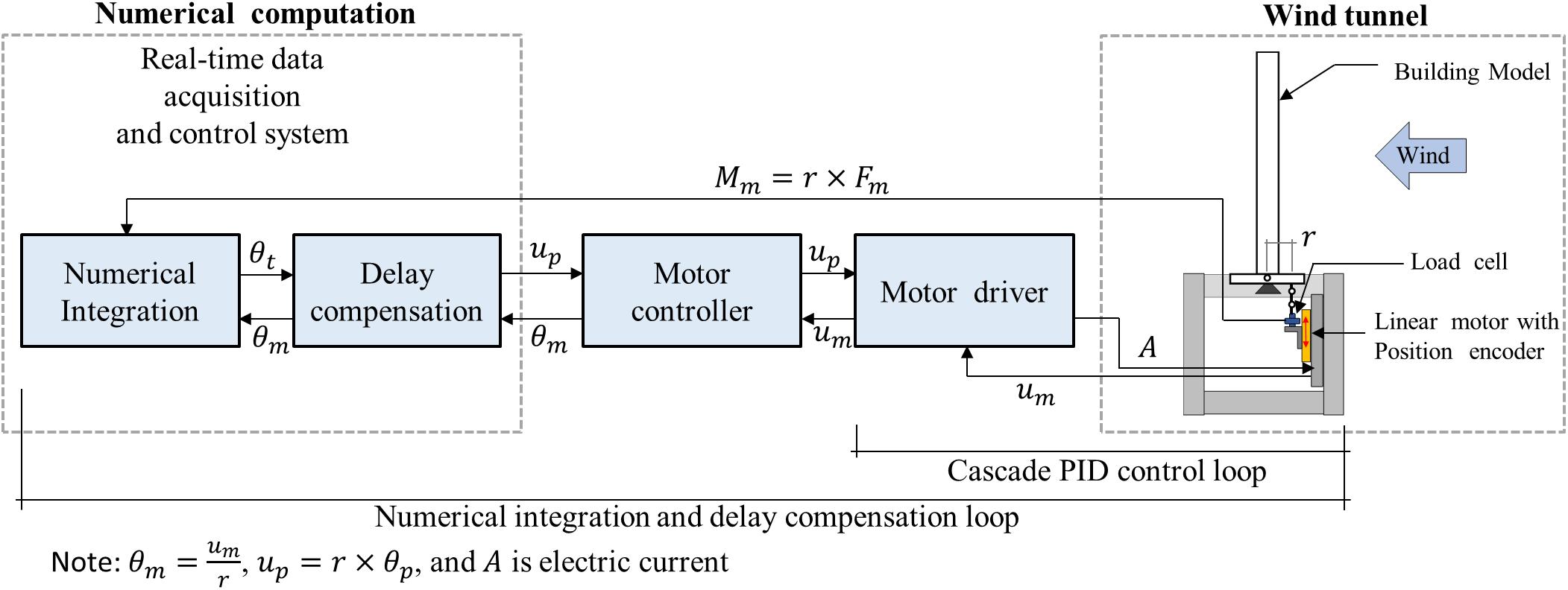
Figure 1. Control loops for the RTAHS.
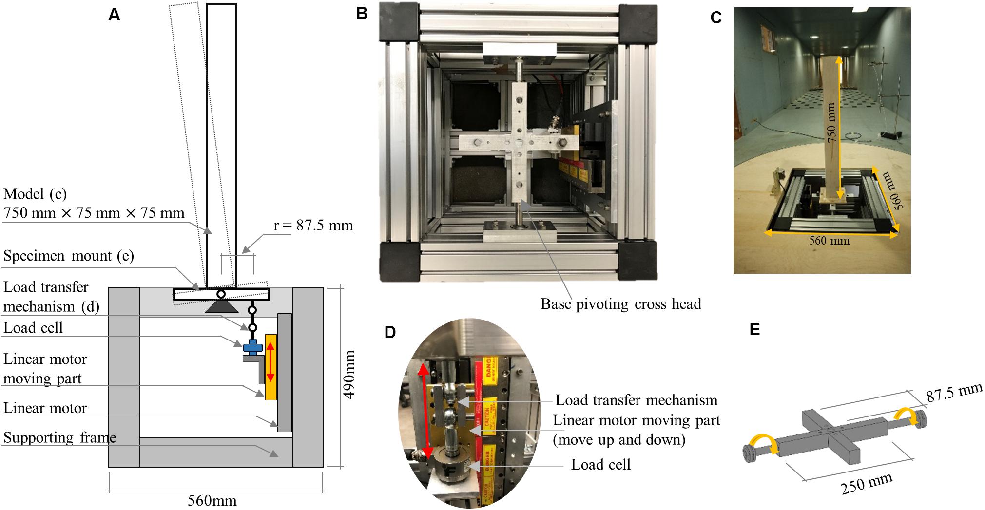
Figure 2. Experimental setup. (A) Schematic configuration of the developed system, (B) plan, (C) physical substructure in wind tunnel, (D) side view of the linear motor moving part, and (E) details of the crosshead.
The following sections present the main components of the proposed RTAHS apparatus.
Experimental Setup
An experimental apparatus is developed to perform the RTAHS for a base-pivoting building model for a crosswind direction. Figure 2A shows the schematic of the developed experimental setup for this study. Figure 2B shows the plan view of the developed system without the model, and Figure 2C shows the developed system in the wind tunnel facility. The main components for the experimental apparatus are as below.
Supporting Frame
A rigid frame is designed to support the linear motor and the base-pivoting system. The frame elements are selected such that they do not develop resonance during the RTAHS. The dimension of the frame is 490 mm in height and 560 mm in width, which is determined based on the geometry of the opening in the wind tunnel. The top of the frame is flush with the wind tunnel floor. The linear motor is mounted to the supporting frame. The specimen mount (crosshead in Figure 2E) is supported on the frame.
Actuation
A linear motor was chosen as an actuator. A rotary motor with a precision gear was also considered as a potential actuator. However, after consulting an equipment manufacturer, it was concluded that a rotary motor was not suitable due to the potential control issue associated with backlash in gear. The direct-drive rotary motor is also possible, but precisely controlling maximum 0.02 rad of rotation angle at maximum 8 Hz would be challenging due to the resolution of the rotary encoder. In addition, implementing a bi-directional pivoting motion in the future upgrade would be challenging when two rotatory motors are used. A load transfer mechanism is designed to transfer the linear motion to a base-pivoting motion, as shown in Figure 2D. The linear motor has a total stroke of 60 mm, peak force of 790 N, continuous force of 176 N, and peak velocity of 2.5 m/s, all of which are far higher than the requirements for the RTAHS. The peak linear velocity corresponds to the angular velocity of 33 rad/s, considering the dimension of the crosshead in Figure 2A.
Sensors
The position of the electric motor is measured with a magnetic encoder with a resolution of 0.001 mm. The base rotation angle is calculated based on the distance from the pivoting point to the point where the load transfer element is mounted (r in Figure 2A). The HFBB method is used to measure wind-induced force in this study. While the HFBB method has its own challenge, as discussed in section “Introduction,” it was advantages as well. For example, the load cell can transfer data at a faster rate than pressure transducers, and the model development is relatively easier than using pressure tabs for an HFPI model. The HFPI model in hybrid simulation also requires the integration of the measured pressures from the pressure taps to calculate the force or moment approximately. This can result in inaccuracies if the geometry of a specimen is complicated. In the proposed design of the experimental setup, the force is measured with a uniaxial tension-compression load cell with a capacity of 445 N. One end of the load cell is connected to the moving part of the linear motor, and the other end is connected to the crosshead through the load transfer element.
Building Model
The building model is constructed with balsa wood. The building model has a height of 750 mm and planner dimensions of 75 mm × 75 mm, which represent a prototype building of 300 m in height and 30 m in width and depth.
Numerical Integration Scheme
This study adopted the central difference method (CDM) to perform numerical integration. There are various numerical integration algorithms developed for hybrid simulations to improve stability and accuracy. The stability resulting from the CDM is not an issue in this study because the smallest period of the base-pivoting single degree of freedom (SDOF) system is sufficiently larger than the integration time step. The stability of CDM depends on the time step and the shortest natural period of the structure. If the shortest period of the structure is τmin and the time step of the integration scheme is Δt, the numerical integration is stable when the following equation is satisfied:
In the current study, the period of the single degree of freedom system is considered 125 ms (i.e., f = 8 Hz), and the time step of the integration scheme considering the processing speed of the real-time controller is 5 ms, which satisfies the above stability criteria.
In the RTAHS, the equation of motion needs to be modified as shown in Eq. (3) because the measured moment includes the moment from the dynamic wind pressure, , and the moment resulting from the acceleration of the specimen and other load transfer elements, . The measured moment is denoted as Mm(t) in Eq. (5)
Then, Eq. (3) can be written in discrete form for step i at time ti = iΔt.
Eq. (6) needs to be solved to predict the displacement in each step. In the CDM, the velocity and acceleration at step i are calculated based on Eqs. (7, 8)
After substituting Eqs. (7, 8) into Eq. (6), the displacement at step i+1, θi+1, can be calculated from the measured moment, Mm,i; numerical mass, IN; damping coefficient, c; structural stiffness coefficient, k; time step, Δt; the previous steps’ displacements θi and θi–1 as shown in Eq. (9)
The displacement predicted with Eq. (9), which is denoted as target displacement, θt, in Figure 1, is modified for delay compensation, which is then transferred to the motor driver. The motor controller in Figure 1 does not have any role in the hybrid simulation other than relaying commands and measurements. The motor controller is required to enable communication from the real-time data acquisition and control system (NI-cDAQ) and the motor driver. A host PC is used between the NI-cDAQ and the motor controller. The data is transferred in real-time from the NI-cDAQ to the motor controller through the host PC.
Delay Compensation
In a real-time hybrid simulation (RTHS), it is essential to impose motion without significant delay. The delay may result in unintended negative damping and a corresponding stability issue, or unintended positive damping. Depending on the dynamic characteristics of the specimen and the actuation system, the delay may be frequency dependent. Besides, if a structural system behaves in the inelastic range (i.e., there are changes in stiffness during a simulation), the initially tuned gain parameters may not work properly. Advanced adaptive delay compensation methods, such as Chae et al. (2013), have been proposed to consider the frequency-dependency or non-linearity in the system.
In the configuration of the testing apparatus proposed for an RTAHS, the selected linear motor has a large continuous force capacity (176 N) in comparison with the actual force required to run the test. The maximum measured peak force was less than 50 N in this research; thus, the specimen-actuator interaction is negligible. In addition, while there is some non-linearity resulting from wind-structure interaction, the overall mass and stiffness of the system can be considered constant. Time delay is observed in preliminary tests of the control scheme, but the delay was constant in the frequency range of interests. Thus, in this study, the inverse time delay compensation method developed by Chen (2007) is adopted, which assumes a constant delay. The method is briefly summarized below, and the method is illustrated in Figure 3B.
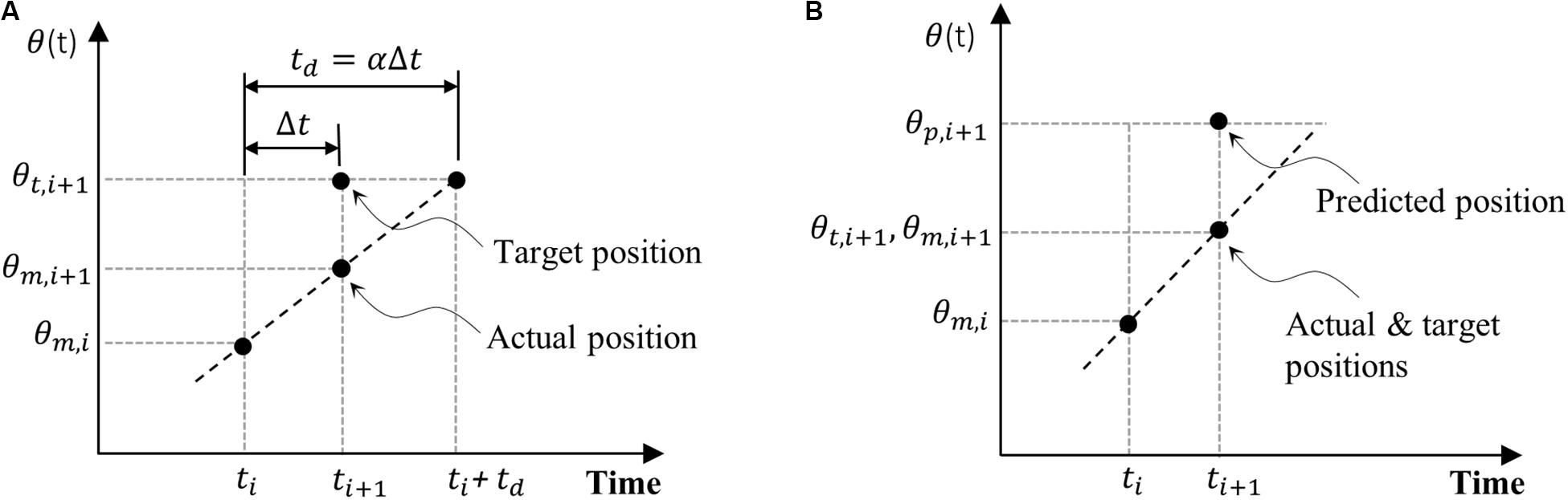
Figure 3. (A) Delay in real-time aeroelastic hybrid simulation, (B) inverse delay compensation.
In the presence of delay, the measured displacement θm, i+1 at time step i+1 can be expressed as
where α is the ratio between the time to reach the target displacement (αΔt in Figure 3A) and the time step Δt, assuming a constant delay. Eq. (10) can be rearranged in terms of the target displacement, θt, i+1.
By applying the first-order discrete Z-transform, the relationship between the target displacement and the measured response can be obtained, as shown in the transfer function in Eq. (12).
where Xm,θ(z) and Xt,θ(z) are the discrete Z-transform of θm, i+1 and θt, i+1, respectively. Note that when there is no delay (i.e., α = 1), the value of the transfer function becomes one. To compensate for the delay, the predicted displacement, θp, i+1, can be imposed on the controller instead of the target displacement, θt, i+1, where the predicted displacement is calculated as:
In a conventional RTHS of structures where the restoring force is a function of the deformation of a specimen, the delay in the actuator’s response leads to negative damping, which can lead to a stability issue. In the case of RTAHS, however, the measured force includes the inertial force term as shown in Eq. (5), which is proportional to acceleration. For an oscillating system, the phase of the acceleration is 180 deg apart (i.e., opposite sign) from the phase of the displacement. Thus, the delay in the actuator’s response leads to the delay in the acceleration response, which in turn leads to a positive damping effect rather than a negative one.
To further elaborate, let us consider an SDOF system with an angular frequency of ωo subjected to steady-state harmonic displacement with an amplitude of θo as defined in Eq. (14). This displacement profile is imposed on a control system; thus, the displacement is denoted as target displacement, θt:
If there is a constant delay of, δt, the measured displacement and acceleration are:
The inertial moment due to the physical mass of the system, , depends on the measured acceleration in Eq. (16). Then, the apparent energy increment per each cycle of motion (i.e., duration of T = 2π/ωo) due to the inertial moment, MI, is,
where MR is the ratio between the experimental inertia mass, IE, and the total inertia mass, I, as defined in Eq. (18) and k is the stiffness of the system as defined in Eq. (1).
As shown in Eq. (17) the delays in the actuator’s response leads to positive damping, i.e., energy dissipation, not negative damping. It is worth noting that a similar expression for a displacement-dependent force (e.g., linear spring) leads to negative damping.
The energy dissipation in Eq. (17) can be expressed as equivalent viscous damping, Ceq. The energy dissipated per cycle by a viscous damping force in a SDOF system oscillating with an amplitude of θo and frequency of ωo can be derived as,
By equating Eqs. (17, 19), one can find an equivalent damping coefficient and corresponding damping ratio, as shown in Eqs. (20, 21), respectively,
Thus, the equivalent damping ratio, ξeq, can be expressed as a function of mass ratio, MR, frequency of the structure, fo, and constant delay, δt, of the actuator-control system. The observed delay from the experiment and the corresponding damping ratio is further discussed in section “Free Vibration Test.”
Cascade PID Control of Linear Motor
The predicted displacement in Eq. (13), θp, i+1, is imposed on the motor driver in Figure 1 after converting the rotary motion to linear motion, i.e., up,i + 1 = θp,i + 1×r. The motor driver controls the linear motor using a cascade PID control. It is the default control structure implemented in the motor drive, and the user can optimize the gain parameters. The cascade PID control includes three different control loops: the position loop, velocity loop and current loop. The current loop acts as the inner loop for the velocity loop, and the velocity loop act as an inner loop of the position loop.
For optimal performance, the control gains need to be tuned. In this study, the gains were calibrated after attaching all physical components, including the model building. After calibration, the system response was observed, as shown in Figure 4. From this figure, it can be observed that the response does not overshoot and monotonically approach the target command. There are 5 ms of delay before the system starts moving. This delay is due to the 5 ms of loop time used in the controller. It took 30 ms to reach the target displacement. After running all tests, the authors learned that the gain parameters could have been further tuned to reduce the 30 ms of delay before the delay compensation was applied.
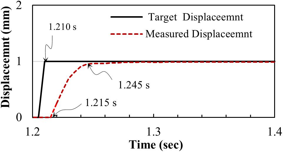
Figure 4. Response of the motor to the pulse signal.
Preliminary Tests for Characterization of Dynamic Properties
Dynamic characteristics of the experimental apparatus and the control system are identified by imposing a white noise displacement profile, cyclic tests, and free vibration tests. A white noise displacement profile is used to identify the delay characteristics. The cyclic tests are used to measure the actual inertia mass of the specimen and the moving parts in the pivoting system. Free vibration tests are performed to evaluate the relationship between the input and output values of frequency and damping.
White Noise Test and Cyclic Test
The white noise signal, which was filtered through a low-pass filter, is used to measure the delay characteristics of the actuator. The input signal is a predefined displacement history, which has a magnitude of 1 mm and a frequency range of 0.1–10 Hz. Note that the numerical integration scheme is not used in these tests because the displacement histories are predefined.
The input displacement histories and the response of the linear motor are used to obtain a transfer function in the form of the Bode plot. The Bode plot of the white noise signal with and without delay compensation technique is presented in Figure 5. The delay for the system without delay compensation (i.e., α = 1) is observed to be 29 ms, which is consistent with the observation from the step response shown in Figure 4. Chen et al. (2009) defined α as the ratio of the actuator delay to the servo controller sampling time (i.e., time step). The actuator delay is defined as the time difference between the time when the compensated command (θp = up/r in Figure 1) is issued and the time when the measured displacement (θm) becomes similar to the compensated command. When the time delay compensation is not applied (α = 1), the target command (θt) is identical to the compensated command as shown in Eq. (13). From the white noise test with α = 1, it was found that the actuator delay was 29 ms. Because the sampling time of the servo controller was 5 ms, the proper value of α is approximately 6.
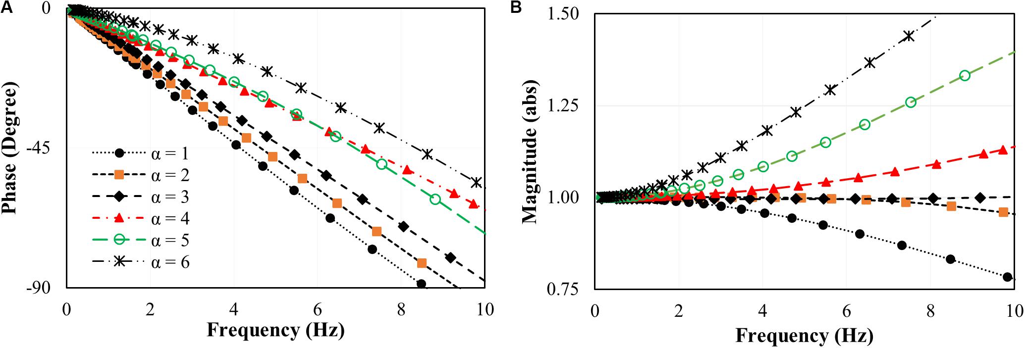
Figure 5. Bode plot of response to white noise signal. (A) Phase angle, and (B) magnitude.
After the first test with α = 1, the inverse delay compensation scheme discussed in section “Delay Compensation” was used with α values ranging from 2 to 6 to observe the performance of the delay compensation scheme. It was observed from the tests that the delay decreases as the value of α increases. However, as the value of α increases, the amplitude error was increasing as a function of frequency. With the α value of 6, the amplitude increases to 146% at the frequency of 8 Hz as shown in Figure 5B. In addition, the delay of 16 ms was still observed with the α value of 6. Thus, with the inverse delay compensation scheme, the maximum value of α is deemed to be 3, as it did not introduce amplitude error that was observed in Figure 5B. At this value of α, the observed delay was 23 ms as shown in Figure 5A, which was not a significant improvement from 29 ms. The delay of 23 ms leads to additional damping, as discussed in section “Apparent Damping,” which was compensated by tuning the numerical damping parameter.
The authors also carried out additional tests with an independent experimental setup. We observed that the inverse delay compensation scheme does not fully reduce the delay and tends to amplify the vibration as the value of α increases. Therefore, it is suggested to adopt a more advanced delay compensation scheme in future tests.
After the installation of the specimen, cyclic tests were also performed to measure the physical mass, IE in Eq. (3). A displacement amplitude of 0.4375 mm was imposed at each frequency, which is equivalent to 1/200 radian of rotation. After the completion of the cyclic tests, the relationship between the RMS value of measured force, Frms, and the RMS value of angular acceleration, was found. The physical mass, IE of the moving part was obtained by using Eq. (22). In this equation, r is the distance in mm of the pivoting point from the load cell, as shown in Figure 2A:
The considered frequency range is 4–8 Hz. The mass moment of inertia from this test is found to be IE = 35,900 kg-mm2. This value is used to perform the free vibration test and the RTAHS.
Free Vibration Tests
Free vibration tests were performed considering a mass ratio, MR, of 0.5 to 20%; the mass ratio is the ratio of physical mass to the total mass as presented in Eq. (18). The frequency ranges from 4 to 8 Hz, and the damping ratio of -1.5 to 0% was considered to run the free vibration tests. Note that negative damping was imposed because of the additional damping introduced by the approximately 23 ms of delay discussed in section “White Noise Test and Cyclic Test.” The free vibration test was performed by applying an initial displacement of 0.875 mm, which is equivalent to 1/100 radian of rotation. The measured force, which includes the inertial component, in Eq. (5), but not wind-induced force, is fed back to the equation of motion.
Figures 6A,B presents the target command predicted by Eq. (9), which is labeled as “Target” in the figure, the predicted command after delay compensation in Eq. (13) which is labeled as “Compensated,” and the measured response for the case with a mass ratio of 5% (MR-7 in Table 1), damping ratio of 0% and a frequency of 6 Hz. It can be observed that even with 0% of the damping ratio, the system shows logarithmic decay due to the additional damping from the delay. In this case, the observed delay of 23 ms is consistent with the delay when α = 3 in Figure 5. From a series of parametric tests summarized in Table 1, however, we found that the delay varies from 14 to 23 ms, and the average delay is 19 ms depending on the test parameters of specified frequency, mass ratio, or damping ratio. The difference between the average delay (19 ms) from free vibration tests and the delay observed from white noise tests with α of 3 (23 ms) is about 5 ms. Further investigation is required to find out the cause of this delay difference. A more robust delay compensation method needs to be implemented in future test.
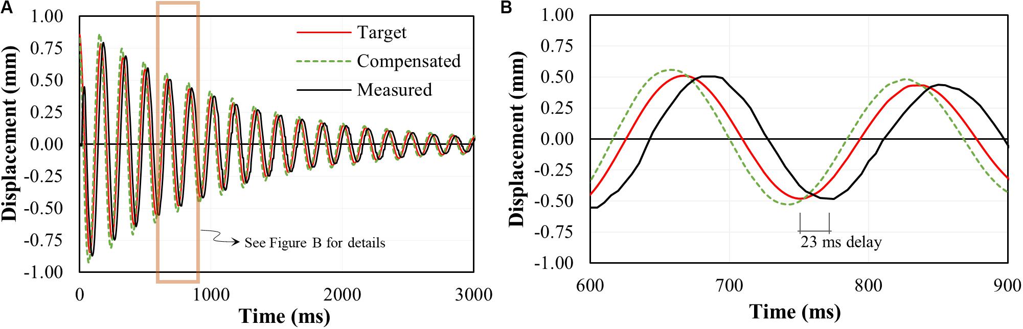
Figure 6. Time history of free vibration test for case (MR−7andξI = 0,f = 6.0Hz). (A) Complete response history, and (B) response history between 600 ms and 900 ms.
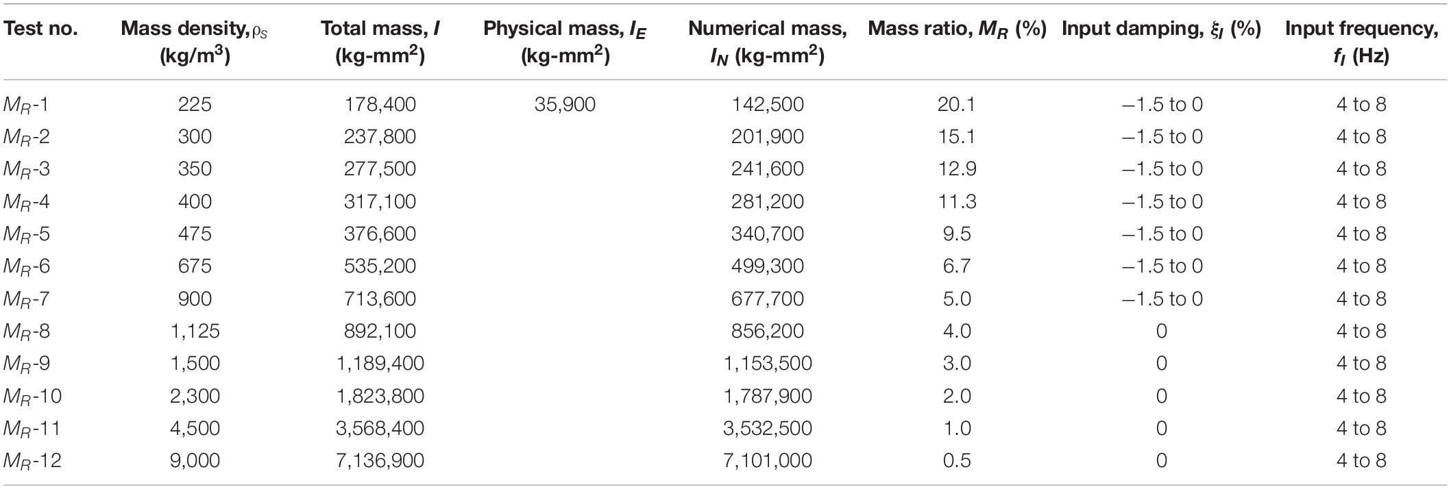
Table 1. Control parameters of free vibration test.
In order to evaluate the dynamic characteristics of the proposed testing apparatus in the presence of the delay, a series of free vibration tests are carried out by using mass ratio, damping ratio and natural frequency as control parameters. In Table 1, the physical mass, IE, is fixed for all tests. The mass density is the average mass density of a high-rise building structure. The typical range of mass density for high-rise buildings varies from 200 to 450 kg/m3. In this study, however, much higher values of mass density are also used to investigate the impact of the mass ratio on the additional damping (i.e., Eq. 21). The total mass in Table 1 is the rotational mass of the scaled model, considering the dynamic similitude law. Then, the numerical mass is defined as the difference between the total mass and the physical mass. After the parametric experiments, the observed apparent frequency and damping ratio of the system are presented in the following subsections.
Apparent Frequency
After completing the free vibration tests, the frequency of the system is evaluated from the measured displacement response. In Table 2, the input frequency, fI, is the frequency defined as the property of the system in Eq. (1). The observed apparent frequencies are listed in the columns with the label fM which is evaluated based on the Fast Fourier Transform (FFT) of the measured response. From this table, it can be observed that with the increase of the mass ratio, the difference of input and output frequency increases. The largest difference between the input and measured frequencies was 6.8%, which was observed from the test cases MR-1 when the input frequency was 6 Hz. For test cases from MR-3 to MR-12 (i.e., mass ratio less than 12.9%), the maximum frequency error is 0.3%. From this observation, it can be concluded that the mass ratio influences the frequency error. If the mass ratio is below a certain threshold (e.g., 12.9% in this study), the frequency error is negligible.
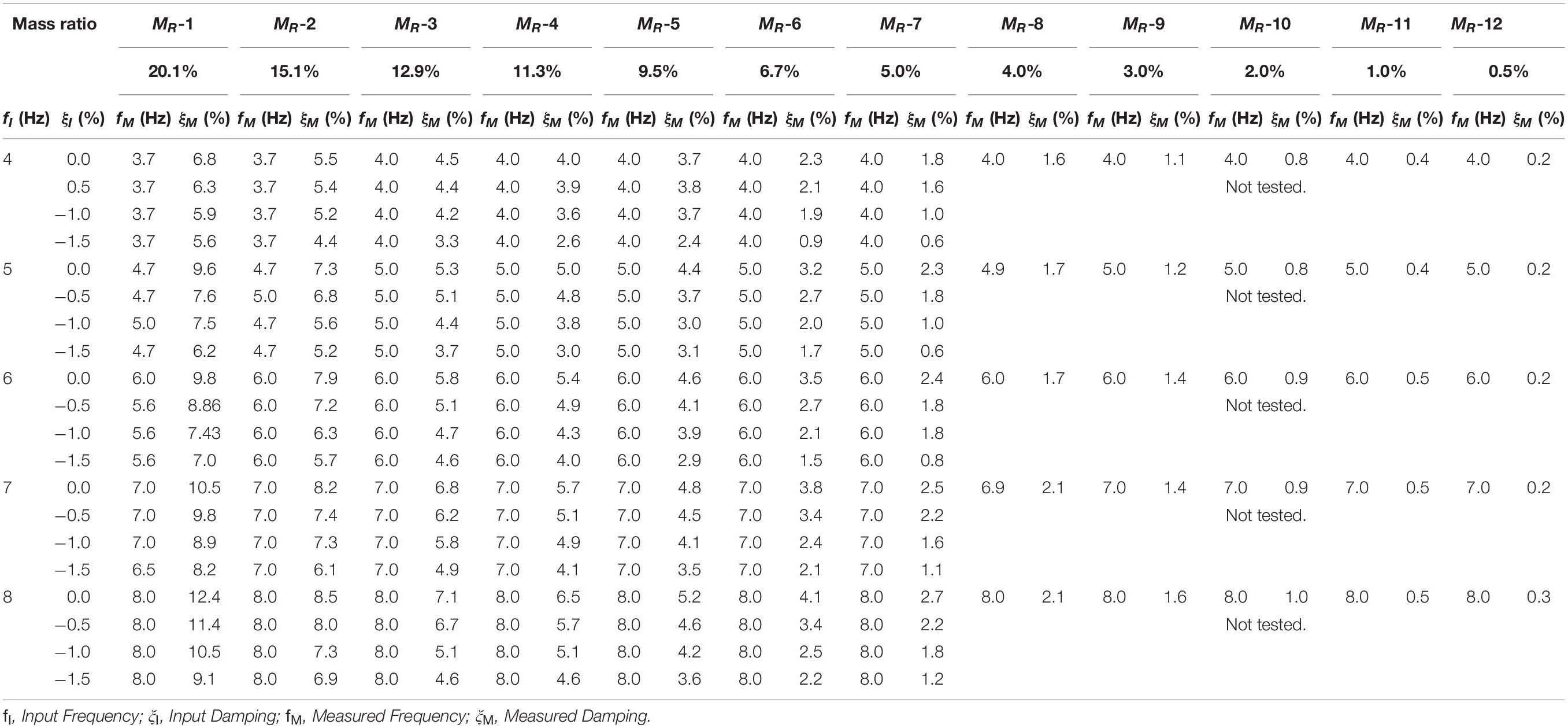
Table 2. Free vibration result.
Apparent Damping
The observed apparent damping ratio is evaluated from the measured displacement signal by assuming logarithmic decay. Table 2 shows the apparent damping ratio for different frequencies, numerically defined damping ratios and mass ratios. Figure 7A shows the relationship between the mass ratio and measured damping ratios. The input damping for this figure is zero, and the input frequencies are 4.0, 6.0, and 8.0 Hz. The predicted damping ratio from Eq. (21), which is calculated based on the time delay of 23 ms observed in the white noise test (as discussed in section “White Noise Test and Cyclic Test”) and the input frequency, is also presented in solid lines. Figure 7A shows that the trend is similar in the measured damping ratio and the predicted damping ratio and that the damping ratio increases as the mass ratio increases. The discrepancy between the measured damping ratio and the predicted damping ratio would have resulted from one or more of the following: the frequency error, an inconsistent delay in each test, energy dissipation from swivel joint, or the numerical evaluation of the damping ratio from the measured time-series data. When the damping ratio is large, the response decays quickly. Thus, using only a few data points to fit the logarithmic decay curve would result in an error estimating the damping ratio.
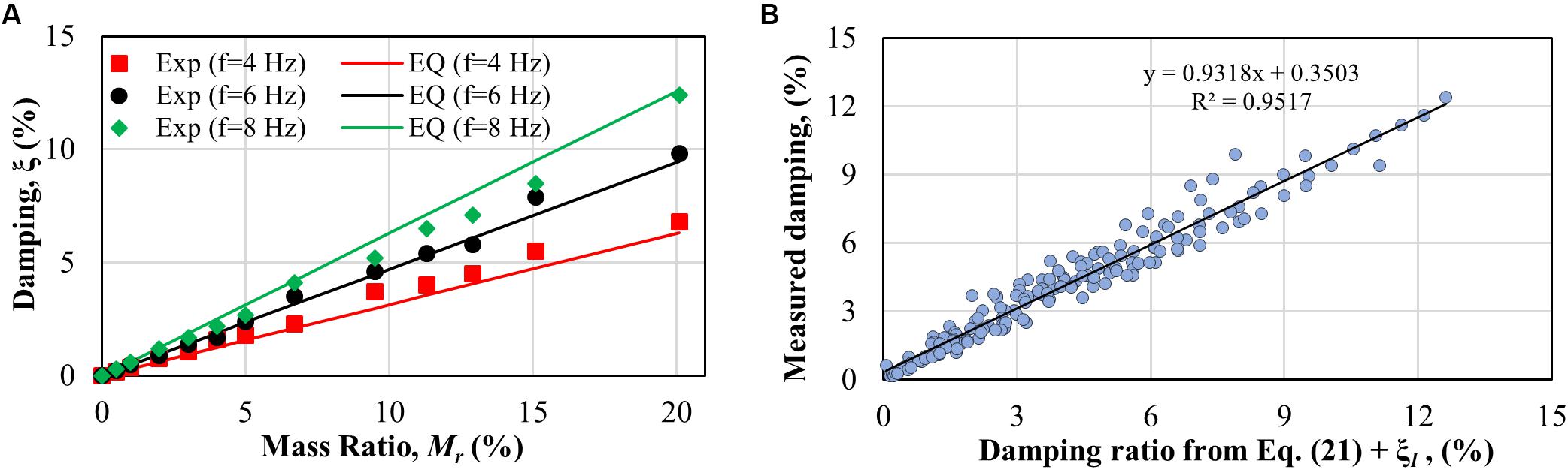
Figure 7. Experimental and calculated damping comparison. (A) Change of damping with mass ratio, (B) comparison of calculated and measured damping.
Figure 7B compares the predicted damping ratio using Eq. (21) added to the input damping ratio, ξI, in Table 2, against the measured damping ratios from all tests. It can be observed from the figure that the predicted and measured damping ratios are well-correlated with an average slope of 0.93. The discrepancy between the predicted and measured damping ratios deserves further investigation, especially after reducing the delay in the actuator’s response and reducing the mass of the moving parts in the experimental apparatus.
Real-Time Aeroelastic Hybrid Simulation (RTAHS)
RTAHS is performed with the building model introduced in section “Experimental Setup.” The building model is a 1:400 scale model of a prototype structure with a height of 300 m. A total of 45 RTAHS tests were conducted by controlling several parameters, as summarized in Table 3. Two mass ratios, 6.7 and 5% were chosen for this study, which corresponds to effective mass density ratios of 551 and 735. These mass density ratios are greater than mass density ratios of typical high-rise buildings. Because the objective of the tests is to validate the hybrid simulation method, rather than evaluating the wind response of a specific building, the effective mass density ratios were deemed appropriate. Because of the presence of the damping introduced in the delay, the damping coefficient in Eq. (1) is adjusted to achieve a target damping ratio. The target damping ratio ξ T(%) for the RTAHS cases R-1, R-2, and R-3 are 1.5, 1.25, and 0.8%, respectively. Three different frequencies, 4.2, 6.0, and 8.0 Hz, are used to perform the RTAHS. The mean wind velocity measurements at the top of the building model are 4, 5, 6, 7, 8, and 9 m/s for cases R-1 and R-2, and 5, 6, and 7 m/s for the R-3 case. The RTAHS is performed by considering open terrain for the considered building.
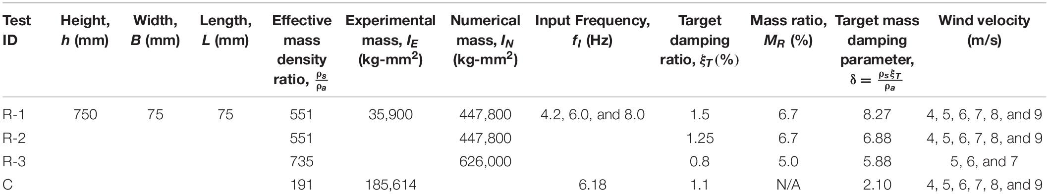
Table 3. Parameters for real-time and conventional aeroelastic hybrid simulation.
The normalized root means square (NRMS) error of the measured displacement is calculated to confirm that the linear motor is achieving the target displacement accurately. In the current RTAHS, most tests have an NRMS error of less than 5%, as shown in Figure 8A. In most cases, the NRMS error is less than 2%, which confirms that the linear motor follows the command without significant error. The displacement history record for an RTAHS case (R-1 with a frequency of 8 Hz and wind velocity 9 m/s) is shown in Figures 8B,C. These figures also confirm that the linear motor follows the target command properly with a certain level of delay.
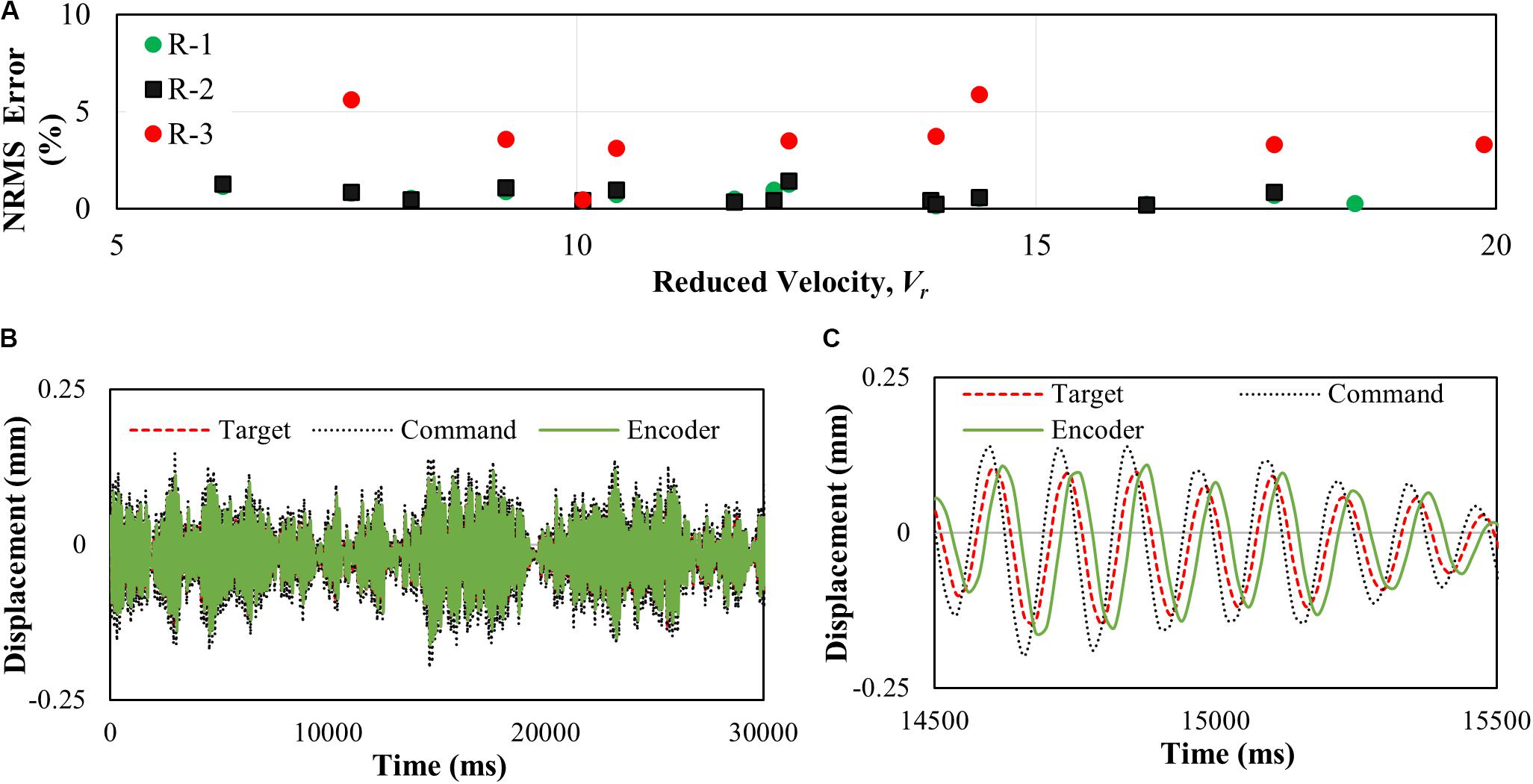
Figure 8. Accuracy of the developed system. (A) Amplitude error, (B) time history for real-time hybrid simulation, (C) zoom-in view of time history for a real-time hybrid simulation.
Validation of the Test Result
In order to validate the RTAHS method, the test results are compared against conventional aeroelastic tests with the same building model, and also against the available test results in Kato and Kanda (2014). The properties of the conventional aeroelastic test specimen are summarized in Table 3. The conventional aeroelastic test was performed by considering an effective mass density, , of 191 where ρa is the density of the air, structural damping ratio, ξ, of 1.1%, and frequency of 6.18 Hz. In the conventional aeroelastic test, two linear springs with stiffness of 0.92 N/mm are fixed to the supporting frame, as shown in Figure 9A. A mass is attached to the rod, which can move vertically to tune the frequency of the model. A magnetic damper based on eddy current damping is attached at the base, which can be adjusted to tune the damping coefficient. The illustration for the overall configuration and experimental setup is shown in Figure 9.
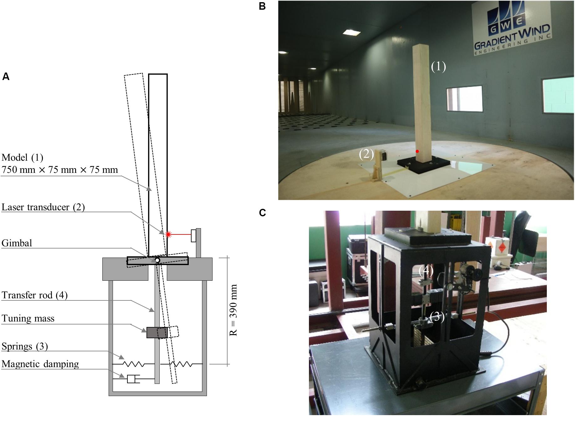
Figure 9. Conventional aeroelastic test for buildings. (A) Schematic configuration, (B) base-pivoting model in wind tunnel, and (C) aeroelastic test rig (the lower part with spring, mass and damper).
The response of a building model under wind load depends on the mass-damping parameter, δ, and the reduced (or normalized) wind velocity. The mass-damping parameter is defined as below:
where ρs is the mass density of the building, ρa is the air density and ξ the structural damping ratio. As shown in Eq. (23), higher damping and higher structural mass lead to a higher mass-damping parameter. Thus, a smaller structural response is expected with a higher mass-damping parameter. The mass-damping parameters, δ, for the conventional aeroelastic test, and R-1 and R-3 of RTAHS are 2.1, 5.88, and 8.27, respectively, whereas the mass-damping parameter of the test results in Kato and Kanda (2014) is 2.0.
The reduced velocity (Vr)is a dimensionless parameter, which is defined as the ratio of the mean wind speed (u) to the frequency (f) and width (b) of the building:
The wind velocity for the conventional aeroelastic tests varies from approximately 4–9 m/s, which corresponds to the reduced velocity, Vr, from 8.61 to 19.41. The vibration amplitude of the model is measured with two laser displacement transducers.
Figure 10 compares the RMS angular response of the specimen from four different test cases. Because the test cases have different characteristic mass-damping parameters, it is difficult to directly compare the absolute values of response from the RTAHS, the conventional test and the results reported in Kato and Kanda (2014). Nevertheless, the tendency of the responses as a function of reduced velocity and as a function of the mass-damping parameter can be qualitatively compared. Because the RTAHS R-1 has a higher mass-damping parameter, it shows little angular vibration amplitude compared to the other three cases.
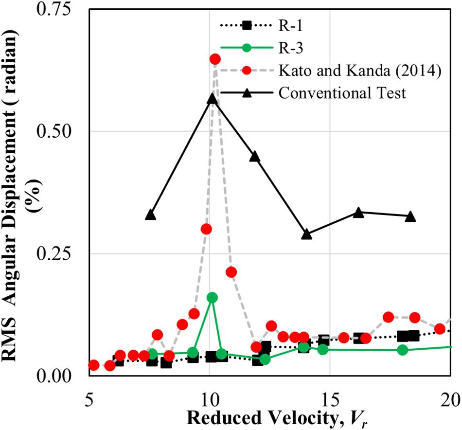
Figure 10. Comparison of angular displacement from RTAHS, conventional aeroelastic tests, and Kato and Kanda (2014).
In the case of conventional tests, the vortex-induced vibration phenomenon is not clearly visible, unlike the results from Kato and Kanda (2014), which have similar mass-damping parameters. In addition, the vibration amplitude of conventional tests is relatively large, not only in the vortex-induced vibration region but also in other wind velocity regions. In order to analyze the conventional test results in detail, the vibration results at the reduced velocity of 10.1 and 11.9 are plotted in Figure 11. Figure 11A shows the measured rotation angle history from the conventional aeroelastic test at a reduced velocity of 11.9. The peak-factor of the vibration at that velocity is 3.2, which is within the range of 3–4 observed in the buffeting response. Thus, it is speculated that the relatively large response of the conventional tests is due to the buffeting response of the specimen. The result at the reduced velocity of 10.1 in Figure 11B shows that the vibration is in an almost steady-state. Because the peak-factor value for this case is 2.5, it seems that the vortex-induced vibration was not fully generated for the conventional aeroelastic test.
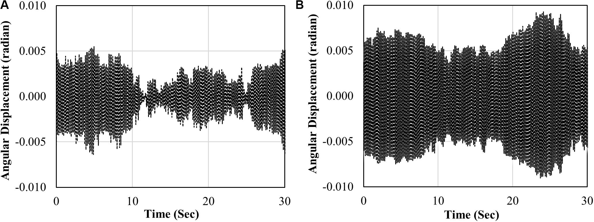
Figure 11. Time series data of the conventional test (A) at the reduced velocity of 11.9 (B) at the reduced velocity of 10.1.
The cases R-1 and R-3 show little response in most regions in comparison with the conventional aeroelastic test due to the high-mass damping parameters. Case R-3 showed a larger response at the reduced velocity of around 10, which coincides with the reduced velocity when the conventional test and the results from Kato and Kanda (2014) showed peak response. This reduced velocity is due to vortex shedding. The reason why vortex-induced vibration did not occur in the R-1 case can be explained by the mass-damping parameter, which is consistent with Cheng et al. (2002), where it was found that the vortex-shedding effect is not manifested when the mass-damping parameters are equal to or greater than 6.28.
The Response Curve for Angular Displacement and Acceleration
Figures 12A,B present the RMS angular displacements and RMS angular acceleration as functions of the reduced velocity, respectively. For the RTAHS test case, as well as R-1 and R-2, the effective mass density ratio of the building is 551. The considered damping ratios for R-1 and R-2 are 1.5 and 1.25%, respectively, as summarized in Table 3. The mass-damping parameter for the R-1 and R-2 is 8.27 and 6.88, respectively. For the case of R-3, the vortex shedding happened at a reduced velocity of 10.1, with the magnitude of the angular displacement being 0.16%. The vortex shedding effect for R-1 and R-2 is not observed in this study since the cases have a higher mass-damping parameter. In buildings with a mass-damping parameter greater than or equal to 6.28, the vortex shedding effect does not occur (Cheng et al., 2002). The maximum angular acceleration observed at the vortex shedding condition is 0.058 rad/sec2 for test case R-3, and at reduced wind speed, it was observed to be 10.1. The RMS angular acceleration is obtained from the RMS angular displacement, using Eq. (25). In this equation, T is the fundamental period of the structure.
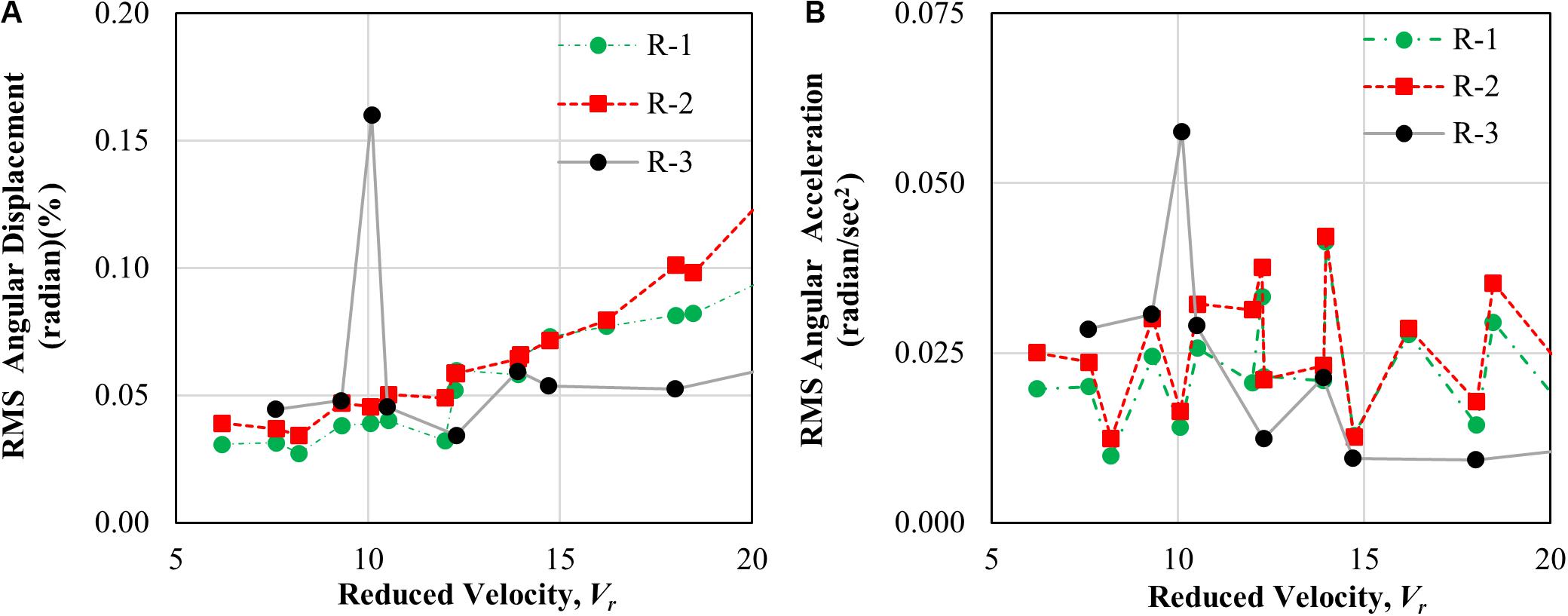
Figure 12. The response curve of the current study. (A) Displacement, (B) acceleration.
Conclusion
This study presents a new design of an experimental apparatus for real-time aeroelastic hybrid simulation of a base-pivoting building model. The experimental apparatus mainly consists of a linear motor, a motor driver, a real-time controller, and transducers. The inverse delay compensation scheme is adopted to reduce the actuator time delay. A series of preliminary tests and RTAHS tests are carried out. The following are the main findings from the tests:
• From white noise tests, the delay in the linear motor was about 29 ms when delay compensation was not used. It is speculated that the constant delay could have been reduced if PID gains were further optimized.
• With the presence of 29 ms of constant delay, the inverse delay compensation scheme was used. The delay was reduced to 23 ms when α = 3, without having an amplitude error. It was expected that when the value of α was 6, the phase and amplitude error should be small. However, the experimental results showed an increase in the amplitude error when the value of α was larger than 3. This observation requires further investigation.
• An expression is derived to relate apparent damping, which results from the delay in the motor’s response, the physical mass of the specimen and the specified natural frequency of the specimen. Unlike conventional substructuring tests of displacement-dependent elements, the result of the delay is an increase in damping ratio. The free vibration tests confirmed that the measured damping ratios are consistent with the derived equation.
• Based on a series of free vibration tests, it was observed that the delay does not impact the frequency of the system when there is a mass ratio of less than 15%.
• RTAHS tests were conducted to validate the developed system. A relatively large mass-damping ratio was used in the tests. There was only one case (R-3) in which the vortex-induced vibration was observed at the reduced velocity of approximately 10, a result consistent with those from the literature. In other cases (R-1 and R-2), the vortex-induced vibrations were not observed due to a higher mass-damping ratio, which is also consistent with the existing literature.
The main contributions of this study are the noble design of the experimental apparatus, as well as the verification and validation of the implemented control schemes. The RTAHS is beneficial over conventional aeroelastic tests as a user can rapidly define the dynamic characteristic of the system. In addition, RTAHS provides additional benefits. For example, the main program can be further extended by implementing tuned mass damper, tuned liquid damper, or any other supplemental damper models, which will allow rapid prototyping of appropriate damping system to control the vibration of a building subjected to wind load. There are a few topics that remain to be investigated in future studies. Some of the following are currently in progress:
• The gains of the controllers need further calibration to make the system more responsive.
• The observed issue in the inverse delay compensation and the variation of delay at different testing parameters needs to be addressed by implementing an advanced delay compensation method.
• Further systematic RTAHS experiments need to be carried out at low mass-damping ratios.
• The configuration shown in Figure 1 includes a redundant motor controller. Research is in progress to simplify the configuration beyond the design presented in this paper.
• It is necessary to expand the experimental setup to model both along-wind and across-wind vibration by using two linear motors.
• While the impact of delay can be compensated by adjusting numerical damping, the impact of delay can be further reduced by optimizing the design of the moving part of the experimental setup to reduce the mass ratio.
Data Availability Statement
All datasets generated for this study are included in the article/supplementary material.
Author Contributions
MM designed the testing apparatus, conducted the tests, and drafted the manuscript. YH contributed to the implementation of the control scheme and configuration of the RTAHS. O-SK and H-KK supervised the research. UJ provided practical advice on aeroelastic tests, proposed a range of testing parameters, and provided supports in fabrication and testing in the wind tunnel facility. All authors contributed to the article and approved the submitted version.
Funding
The equipment for the research was funded by the Natural Sciences and Engineering Research Council of Canada (NSERC) Research Tools and Instruments grant (RTI-2017-00471). The students and the tests at the wind tunnel facility were funded through the Ontario Centres of Excellence (OCE) VIP I Grant (#30735) and NSERC Engage Grant (EGP 530176-18). MM was partially funded by the NSERC Alexander Graham Bell Canada Graduate Scholarship-Doctoral (CGS D).
Conflict of Interest
UJ was employed by the company Gradient Wind Engineering Inc.
The remaining authors declare that the research was conducted in the absence of any commercial or financial relationships that could be construed as a potential conflict of interest.
Acknowledgments
We are grateful to Mr. Marco Aulla Villacres and Mr. Junyan Xiao, Ph.D. students at the University of Toronto, for providing supports during the testing at the GWE wind tunnel facility. We would like to acknowledge the technical staff at the Gradient Wind Engineering for their assistance during the RTAHS tests.
References
Ahmadizadeh, M. (2007). Real-Time Seismic Hybrid Simulation Procedures for Reliable Structural Performance Testing. Ph.D. thesis, State University of New York, Buffalo, NY.
Al-subaihawi, S., Kolay, C., Marullo, T., Ricles, J. M., and Quiel, S. E. (2020). Assessment of wind-induced vibration mitigation in a tall building with damped outriggers using real-time hybrid simulations. Eng. Struct. 205:10044. doi: 10.1016/j.engstruct.2019.110044
Aly, A. M. (2013). Pressure integration technique for predicting wind-induced response in high-rise buildings. Alexandria Eng. J. 52, 717–731. doi: 10.1016/j.aej.2013.08.006
Amin, J. A., and Ahuja, A. K. (2010). Aerodynamic modifications to the shape of the buildings: a review of the state-of-the-art. Asian J. Civ. Eng. 11, 433–450.
Botelho, R. M., and Christenson, R. E. (2017). “Dynamics of coupled structures,” in Proceedings of the 35th IMAC, A Conference and Exposition on Structural Dynamics, eds M. S. Allen, R. L. Mayes, and D. J. Rixen (Cham: Springer International Publishing), 4., doi: 10.1007/978-3-319-54930-9
Chae, Y., Kazemibidokhti, K., and Ricles, J. M. (2013). Adaptive time series compensator for delay compensation of servo-hydraulic actuator systems for real-time hybrid simulation. Earthq. Eng. Struct. Dyn. 42, 1697–1715. doi: 10.1002/eqe.2294
Chen, C. (2007). Development and Numerical Simulation of Hybrid Effective Force Testing Method. Ph.D. thesis, Lehigh University, Bethlehem, PA.
Chen, C., Ricles, J., Marullo, T., and Mercan, O. (2009). Real-time hybrid testing using the unconditionally stable explicit CR integration algorithm. Earthq. Eng. Struc. Dyn. 38, 23–44. doi: 10.1002/eqe.838
Chen, C., Ricles, J. M., Karavasilis, T. L., Chae, Y., and Sause, R. (2012). Evaluation of a real-time hybrid simulation system for performance evaluation of structures with rate dependent devices subjected to seismic loading. Eng. Struct. 35, 71–82. doi: 10.1016/j.engstruct.2011.10.006
Cheng, C. M., Lu, P. C., and Tsai, M. S. (2002). Acrosswind aerodynamic damping of isolated square-shaped buildings. J. Wind Eng. Ind. Aerodyn. 90, 1743–1756. doi: 10.1016/S0167-6105(02)00284-2
Christenson, R., Lin, Y., Emmons, A., and Bass, B. (2008). Large-scale experimental verification of semiactive control through real-time hybrid simulation. J. Struct. Eng. 134, 522–534. doi: 10.1061/(ASCE)0733-94452008134:4(522)
Dragoiescu, C., Garber, J., and Kumar, K. S. (2006). A comparison of force balance and pressure integration techniques for predicting wind-induced responses of tall buildings. Struct. Congr. 2006, 1–10. doi: 10.1061/40889(201)14
Duthinh, D., and Simiu, E. (2011). The use of wind tunnel measurements in building design. Wind Tunnels and Experimental Fluid Dynamics Research. 281–300. doi: 10.5772/18670
Elshaer, A., Bitsuamlak, G., and El Damatty, A. (2015). “Vibration control of tall buildings using aerodynamic optimization,” in Canadian Congress of Applied Mechanics, At London, ON, doi: 10.13140/RG.2.1.1703.3120
Guo, J. W. W., Ashasi-Sorkhabi, A., Mercan, O., and Christopoulos, C. (2017). Real-time hybrid simulation of structures equipped with viscoelastic-plastic dampers using a user-programmable computational platform. Earthq. Eng. Eng. Vib. 16, 693–711. doi: 10.1007/s11803-017-0408-7
Huang, X., and Kwon, O.-S. (2018). A generalized numerical/experimental distributed simulation framework. J. Earthq. Eng. 24, 682–703. doi: 10.1080/13632469.2018.1423585
Kammula, V., Erochko, J., Kwon, O., and Christopoulos, C. (2014). Application of hybrid-simulation to fragility assessment of the telescoping self-centering energy dissipative bracing system. Earthq. Eng. Struct. Dyn. 43, 811–830. doi: 10.1002/eqe.2374
Kanda, M., Kawaguchi, A., Koizumi, T., and Maruta, E. (2003). A new approach for simulating aerodynamic vibrations of structures in a wind tunnel—development of an experimental system by means of hybrid vibration technique. J. Wind Eng. Ind. Aerodyn. 91, 1419–1440. doi: 10.1016/j.jweia.2003.07.002
Kanda, M., Koizumi, T., and Maruta, E. (2006). Numerical integration scheme for hybrid vibration technique. J. Wind Eng. 31, 1–14. doi: 10.5359/jwe.31.1
Kareem, A., Kijewski, T., and Tamura, Y. (1999). Mitigation of motions of tall buildings with specific examples of recent applications. Wind Struct. An Int. J. 2, 201–251. doi: 10.12989/was.1999.2.3.201
Kato, Y., and Kanda, M. (2014). Development of a modified hybrid aerodynamic vibration technique for simulating aerodynamic vibration of structures in a wind tunnel. J. Wind Eng. Ind. Aerodyn. 135, 10–21. doi: 10.1016/j.jweia.2014.09.005
Kim, W., Yi, J., Tamura, Y., and Ohtake, K. (2016). Aerodynamic Damping of Helical Shaped Super Tall Building. Jeju Island: Advance in Civil, Environmental, and Material Research (ACEM 16)).
Kwon, O.-S., Kim, H.-K., Jeong, U. Y., Hwang, Y.-C., and Moni, M. (2019). “Design of experimental apparatus for real-time wind-tunnel hybrid simulation of bridge decks and buildings,” in Proceedings of ASCE Structures Congress (Orlando, FL), 235–245. doi: 10.1061/9780784482247.022
Mendis, P., Ngo, T., Haritos, N., Hira, A., Samali, B., and Cheung, J. (2007). Wind loading on tall buildings. EJSE Spec. Issue Load. Struct. 3, 41–54.
Mercan, O., and Ricles, J. M. (2009). Experimental studies on real-time testing of structures with elastomeric dampers. J. Struct. Eng. 135:1124. doi: 10.1061/(ASCE)0733-94452009135:91124
Mojiri, S., Kwon, O., and Christopoulos, C. (2019). Development of a ten-element hybrid simulation platform and an adjustable yielding brace for performance evaluation of multi-story braced frames subjected to earthquakes. Earthq. Eng. Struct. Dyn. 48, 749–771. doi: 10.1002/eqe.3155
Mortazavi, P., Huang, X., Kwon, O., and Christopoulos, C. (2017). Example Manual for University of Toronto Simulation (UT-SIM) Framework. An open-source framework for Integrated Multi-Platform Simulations for Structural Resilience, 2nd Edn. Toronto, ON: University of Toronto.
Nishi, M., and Kanda, M. (2010). “Application of hybrid experimental technique for simulating aerodynamic vibration of structures in a wind tunnel,” in The Fifth International Symposium on Computational Wind Engineering, Chapel Hill, NC.
Pozzuoli, C. (2012). Aeroelastic Effects on Tall Buildings: Performance-Based Comfort Analysis. Ph.D. Thesis, University of Braunschweig, Braunschweig.
Schellenberg, A. H., Mahin, S. A., and Fenves, G. L. (2009). “Advanced implementation of hybrid simulation,” in Pacific Earthquake Engineering Research Center, (Berkeley, CA: University of California).
Solum, V. R. (2017). Real-Time Hybrid Model Testing. Trondheim: Norwegian University of Science and Technology.
Sullivan, P. P. (1977). Aeroelastic Galloping of Tall Structures in Simulated Winds. Vancouver, BC: University of British Columbia.
Thepmongkorn, S., Kwok, K. C. S., and Lakshmanan, N. (1999). A two-degree-of-freedom base hinged aeroelastic (BHA) model for response predictions. J. Wind Eng. Ind. Aerodyn. 83, 171–181. doi: 10.1016/s0167-6105(99)00070-7
Wang, X., Kim, R. E., Kwon, O., Yeo, I., and Ahn, J. (2019). Continuous real-time hybrid simulation method for structures subject to Fire. J. Struct. Eng. 145:04019152. doi: 10.1061/(ASCE)ST.1943-541X.0002436
Wu, T., Li, S., and Sivaselvan, M. (2019). Real-time aerodynamics hybrid simulation: a novel wind-tunnel model for flexible bridges. J. Eng. Mech. 145, 1–11. doi: 10.1061/(ASCE)EM.1943-7889.0001649
Wu, T., and Song, W. (2019). Real-time aerodynamics hybrid simulation: wind-induced effects on a reduced-scale building equipped with full-scale dampers. J. Wind Eng. Ind. Aerodyn. 190, 1–9. doi: 10.1016/j.jweia.2019.04.005
Xu, Y. L., and Kwok, K. C. S. (1993). Mode shape corrections for wind tunnel tests of tall buildings. Eng. Struct. 15, 387–392. doi: 10.1016/0141-0296(93)90042-3
Zhao, X., Ding, J. M., and Sun, H. H. (2011). “Structural design of Shanghai tower for wind loads.” in The Twelfth East Asia-Pacific Conference on Structural Engineering and Construction, Procedia Eng. 14, 1759–1767. doi: 10.1016/j.proeng.2011.07.221
Zhou, Y., Kareem, A., and Gu, M. (2002). Mode shape corrections for wind load effects. J. Eng. Mech. 128, 15–23. doi: 10.1061/(asce)0733-9399(2002)128:1(15)
Zhou, Y., and Kareem, A. (2003). Aeroelastic balance. J. Eng. Mech. 129, 283–292. doi: 10.1061/(ASCE)0733-9399(2003)129:3(283)
Keywords: real-time aeroelastic hybrid simulation, RTAHS, base pivoting model, wind tunnel test, high-rise building
Citation: Moni M, Hwang Y, Kwon O-S, Kim H-K and Jeong UY (2020) Real-Time Aeroelastic Hybrid Simulation of a Base-Pivoting Building Model in a Wind Tunnel. Front. Built Environ. 6:560672. doi: 10.3389/fbuil.2020.560672
Received: 09 May 2020; Accepted: 18 August 2020;
Published: 22 September 2020.
Edited by:
Vasilis K. Dertimanis, ETH Zürich, SwitzerlandReviewed by:
Xiaoyun Shao, Western Michigan University, United StatesBrian M. Phillips, University of Florida, United States
Copyright © 2020 Moni, Hwang, Kwon, Kim and Jeong. This is an open-access article distributed under the terms of the Creative Commons Attribution License (CC BY). The use, distribution or reproduction in other forums is permitted, provided the original author(s) and the copyright owner(s) are credited and that the original publication in this journal is cited, in accordance with accepted academic practice. No use, distribution or reproduction is permitted which does not comply with these terms.
*Correspondence: Oh-Sung Kwon, b3Mua3dvbkB1dG9yb250by5jYQ==