 Vasantsingh Pardeshi
 Sanjay Nimbalkar
 Hadi Khabbaz
94% of researchers rate our articles as excellent or good
Learn more about the work of our research integrity team to safeguard the quality of each article we publish.
Find out more
ORIGINAL RESEARCH article
Front. Built Environ., 13 February 2020
Sec. Transportation and Transit Systems
Volume 6 - 2020 | https://doi.org/10.3389/fbuil.2020.00003
This article is part of the Research TopicGeotechnical Innovation for Transport InfrastructuresView all 12 articles
The gravel loss is a major limitation for unsealed roads and it needs major maintenance annually. The continual process of gravel loss leads to the unsustainability of these roads. The unsealed road management faces several issues, viz., difficulty to forecast behavior, huge data collection needs, and a vulnerability in the service and maintenance practices. The quality of gravel material also plays a major role in the process of gravel loss. In view of the aforementioned, appropriate revisions to ARRB material specifications are proposed in this study. The gravel material as per modified ARRB specifications is used on the unsealed road network in the Scenic Rim Regional Council in the state of Queensland. Gravel loss monitoring stations were established over the entire region in order to assess the gravel loss and the implication of using a better quality of gravel material. This study discusses the gravel loss monitoring approaches, data analyses, and improved material specification for gravel. It is found that the modified gravel used on unsealed road performs better than conventionally used gravel.
Unsealed roads are the economic backbone of Australia that depends on mining, farming, and forestry. The significant concerns across many councils about unsealed roads are related to dust, potholes, and either slippery road after wet weather or loose stones after a long period of dry weather. For about 500,000 km length of unsealed roads in Australia, approximate maintenance cost per year is 1B AUD (de Percy, 2018). Scenic Rim Regional Council's annual maintenance budget on the unsealed road is about 2M AUD per year [Scenic Rim Regional Council (SRRC), 2018].
The problems associated with these roads are gravel loss, shape loss, and rideability. These issues are the result of deterioration factors: inadequate drainage capacity, dust, corrugations, potholes, ruts, loose gravel, and frost damage. Alzubaidi and Rolf (2002) reported the systems for rating unsealed roads in Sweden, Finland, Canada, USA, New Zealand, and Australia. Linard (2010) used the System Dynamics Modeling (SDM)-based pavement management model, which is using the Australian Road Research Board (ARRB) research for pavement deterioration and rehabilitation of unsealed roads. Henning et al. (2008, 2015) developed a framework for the maintenance of unsealed roads. They point out that the authorities did not commonly use prevailing asset management systems due to resource-demanding and misleading of the actual conditions. It was demonstrated that dependence on condition data collection could be limited by the use of the material properties of surface aggregates to predict surface performance. The study used historical maintenance records and visual inspection to predict the rate and mode of failure. In addition, Henning et al. (2008) proposed the inclusion of new performance indicators, shape loss, and slope loss, to predict the gravel loss model. Van Zyl (2011) identified a large number of variables influencing the deterioration of unsealed roads. These variables pose difficulty in the development of a reliable model based on statistics of the available data.
The Paige-Green (1989) concept is widely used in a number of design guidelines including the Austroads Part 6 and the TRH 20 Unsealed Roads Design Construction and Maintenance. Ellis and Andrews (2013) concluded the optimized gravel selection on a network basis. Tim and Choummanivong (2016) established the first countrywide Australian local road deterioration model with collaborative effect of 236 road agencies. Those models were developed by analyzing the results of a long-term monitoring program covering 500 sealed and 100 unsealed local road sites in various traffic and climatic environment in Australia. Uys (2011) selected various internationally recognized gravel loss deterioration models to compare the predicted gravel loss with the actual measurements. Tim and Choummanivong (2016) proposed Road Deterioration (RD) and Work Effects (WE) models. The Local Road Deterioration Study (LRDS) commenced during 2000 has produced RD models that can be readily incorporated into Pavement Management System (PMS). Tim and Choummanivong (2016) considered RD models catering for roughness, gravel loss of surface, and shape loss of pavement as well as interim WE model considering the impact of light and medium grader blading and granular resheeting.
In Australia and New Zealand, the outcome from models and research so far is the development of the “Unsealed Roads Manual, Guidelines to Good Practice,” 3rd edition (Giummarra, 2009), which covers management procedures and practices for both the Australian and New Zealand unsealed road network. ARRB has clearly indicated that unsealed roads are presently managed with a few technical input. Due to lack of technical input, the full benefit is not yet realized from the available funding. The “Unsealed Roads Tactical Asset Management Manual” (Henning, 2015) developed in New Zealand is another valuable document. Ellis and Andrews (2013) used the “Unsealed Roads Tactical Asset Management Manual” as a beginning argument and developed a comprehensive strategic forecasting tool for the management of unsealed road networks. This manual emphasizes substantial dependence on rigorous data collection.
Most of the studies reported the complexity in accurate prediction of deterioration models for unsealed roads due to a large number of variables involved. Managing unsealed roads frequently encompasses operational issues, because unsealed roads change quickly and when defects are evident, they must be resolved within a short response period. Due to this, the most routine and cyclic maintenance are programmed according to routine inspections and experience from road operators. However, long-term maintenance activities such as re-graveling and surfacing of these roads need a more sophisticated process that includes predictive models (Paige-Green, 2007). A most important consideration during these analyses involves the economic assessment of diverse maintenance options and timings of intervention. A typical Unsealed Road Management issue is identified as (i) difficulty to forecast behavior, (ii) significant data collection needs, and (iii) variability in the level of service and maintenance practices. Based on the review of available literature, research gaps are identified as follows: (i) requirement to develop better material specification by considering local conditions, (ii) developing Martin's model further for localized condition, (iii) including effects of proper maintenance and effects of blading after the use of better specified material, and (iv) establishing better correlation between gravel loss and rough meter based on modified gravel specification.
Scenic Rim Regional Council (SRRC) maintains an extensive road network of sealed and unsealed roads. The Council provides a road network of 1,816 km, which consists of 53% of the unsealed road networks [(Scenic Rim Regional Council (SRRC), 2018)]. On 30 and 31st March 2017, the rainfall produced by Cyclone Debbie and the cold front meeting over the SRRC ranged from 350 mm in the West of the Scenic Rim region to 800 mm in the East of the Scenic Rim region in a 24 h period. The annual average rainfall for Scenic Rim was 892 mm (Cryna weather station). The 24 h flood event was approximately equal to the annual rainfall. Road drainage is not designed to withstand this level of rainfall in such a short period of time. Figure 1 shows the Scenic Rim Regional Council and adjoining council area.
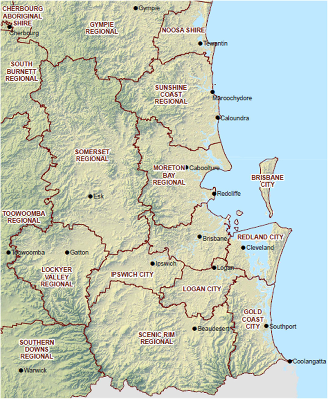
Figure 1. Scenic Rim and surrounding Council in South East Council, Queensland (map reproduced from the Department of Local Government, Queensland website).
SRRC has a planned maintenance schedule resulting in a fairly well-maintained gravel road network. Prior to the cyclone Debbie event, SRRC contracted a private company, IMG to rate all the roads in the region. The majority of the unsealed roads have been rated as three (better) on a 1–5 scale, where 1 is excellent. In many instances, the damage is not immediately apparent as there is no evidence of destructive damage (washes, slips, major erosion). The damage is in the loss of surface material across the entire road surface, loss of shape, loss of fines, and washes in wheel tracks. The volume of water on the roads in a short period has resulted in surface erosion of almost all unsealed roads to some extent. By using the recent information prior to the flood and the information from data collected, the range of restoration treatments proposed are a minimum of a medium grade, a heavy grade with a 50 or 75 mm top-up, and a heavy grade with a 100 mm top or 100 mm resheet and a full 150 mm resheet.
There are 986 unsealed road sections, ~861 km in length, in the Scenic Rim region. Due to a large amount of gravel road involved and many roads now getting resheeted, the SRRC has initiated gravel road-related research project. Figure 2 represent locations of Gravel Loss monitoring stations. The aim of this project is to enhance the existing gravel material specification, measure gravel loss, and calibrate the existing gravel loss models. Based on the developed gravel road maintenance strategy, it is clear that the improved gravel loss models are suitable to the SRRC area.
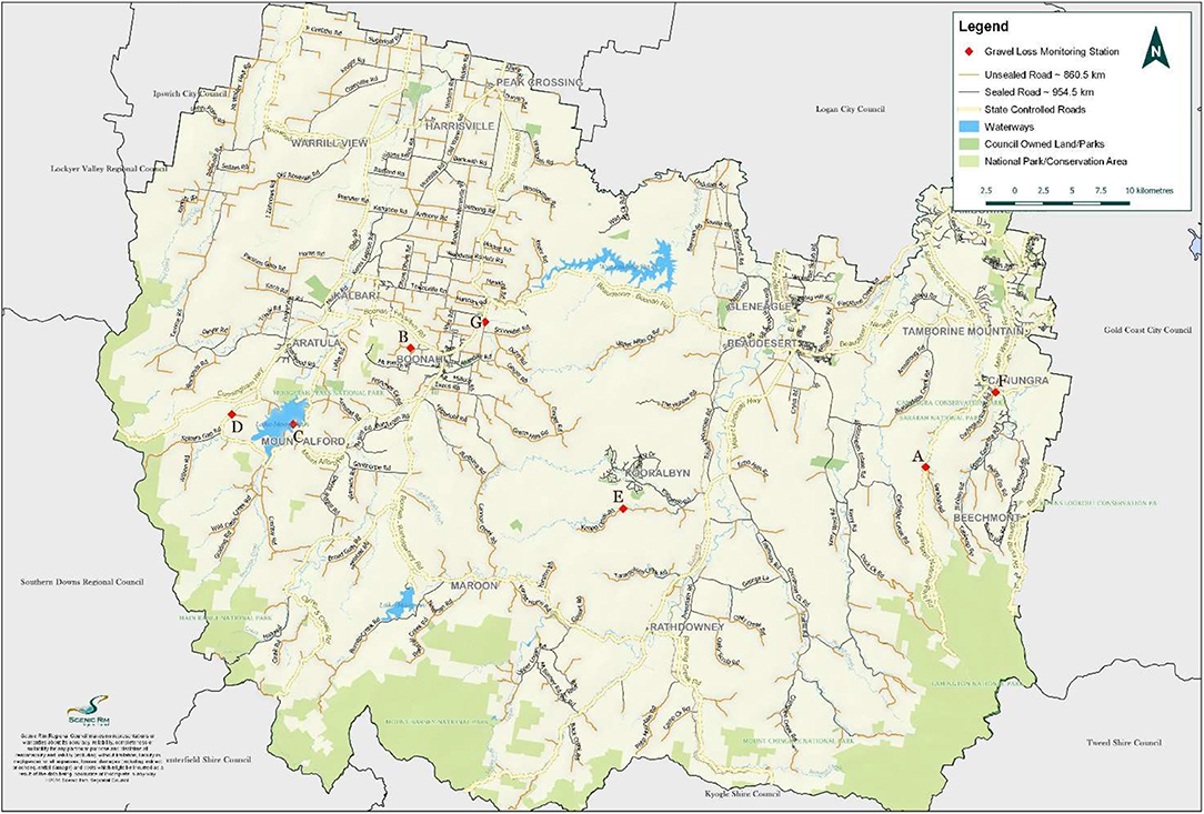
Figure 2. Locations of gravel loss monitoring stations.
Various past studies on gravel road performance have argued that most existing international gravel loss prediction models are unable to capture the intangible characteristics of the locality. Also, the proper handling with inconsistency in gravel materials and climate is not captured. Uys (2011) reported that gravel loss prediction models of South Africa were neither accurate nor transferable due to their local influences. The international prediction models assessed inaccurate gravel loss, re-graveling quantity, and design inputs for estimation of gravel layer thickness, whereas the pavement management theory is based on the precise prediction rate of roadway deterioration.
Various factors such as traffic, weather, material property, the geometry of road, and maintenance practices affect gravel loss. In this study, straight and flat roads are considered (i.e., exclude roads with varying vertical geometry). Three factors, viz., material properties, traffic, and weather condition, are considered and their impacts will also be assessed.
The primary maintenance activities of unsealed roads are grading and resheeting. The frequencies at which grading and resheeting should be applied depending on the economic trade-off between the costs of the grading/resheeting and the benefit to be gained from reducing road-user costs (Paterson, 1991). The loss of gravel material is caused by natural weathering and friction/whip-off from vehicles (Paige-Green, 1989). Most of the gravel loss forecast models enumerated that the rate of gravel loss is a variable of the traffic, road geometry, material properties, and weather. The forecast of the expected gravel loss from a gravel road is significantly important for unsealed road design and maintenance planning, as graveling and re-graveling operations are quite expansive procedures (Paige-Green, 1989). The selection of gravel loss prediction model is based on the optimal re-graveling schedule for effective maintenance management of unsealed roads.
For a management model, the life cycle of unsealed road deterioration and maintenance can be represented by the extents of material loss over time (Paterson, 1991). The mean gravel surfacing material design thickness tends to be reduced progressively under the action of traffic and climate-related deterioration. This reduction in thickness, by keeping other variables constant, may vary with material characteristics and the effectiveness of maintenance practice, until it reaches the minimum depth that shall trigger re-graveling, and then the cycle repeats itself (Paterson, 1991).
Although it has limitations, the gravel loss measurement is among the tools available for implementing maintenance management goals in terms of depletion rate of gravel loss. Therefore, knowledge regarding rate of gravel loss is crucial to an accurate and ideal decision on its re-graveling cycle (Mwaipungu and Allopi, 2014). Bannour et al. (2019) concluded that HDM-4 pavement deterioration models are insufficient to develop an optimal maintenance management strategy for road networks in Morocco.
The predictions from four different gravel loss models are compared with actual measured gravel loss in the field (see Figure 3). These models include (i) the HDM-4 gravel loss deterioration model, (ii) the TRH 20 gravel loss deterioration model, (iii) the Australian GL model (i.e., ARRB model) proposed by Martin et al. (2013), and (iv) the Brazilian gravel loss deterioration model. These four models are more relevant to this study due to the similarity in variables and resemblance to SRRC conditions. To obtain the predicted GL, the input parameters for traffic data, rainfall, and material quality (plasticity and grading values) used are the same for all the models. Percentage differences were calculated for selected stations due to the availability of level data for those stations. The median percentage difference in GL for selected stations was 2% between the actual and ARRB models. There were significant differences between the other three models and actual GL median values. The ARRB model is used for further analysis as it is with least differences with actual GL and is more suitable for Australian conditions. More details of these models are listed below.
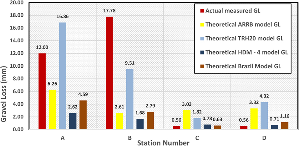
Figure 3. Comparison between the actual and theoretical estimation of gravel loss.
where AGL is the predicted annual material loss (mm/year), RF is average rise and fall of the road (m/km), MMP is mean monthly precipitation (mm/month), AADT is annual average daily traffic (veh/day), KT is the traffic-induced material whiff-off coefficient, and kgl is gravel material loss calibration factor.
To derive the GL values using this model kgl, KT was derived based on actual traffic volume, material quality, and weather data. Also, roads with no curvature were selected for comparison. The gravel loss is calculated using HDM-4 gravel loss deterioration model as:
where GL is the gravel loss (mm) and D is time period under consideration in hundreds of days (days/100).
where ADT is the average daily traffic (total number of vehicles/day), N is Weinert N value, P26 is the percentage by mass of material passing a 26.5 mm sieve, and PF is the product of plastic limit and percentage passing a 0.075 mm sieve.
To derive the GL values using this model, N was assumed 4 based on Australian Climatic conditions. The value of gravel loss is calculated from the following equation:
where MMP is the mean monthly precipitation (mm/month), PF is the plasticity factor (= PI × P0.075), P0.075 is the percentage by mass of material passing a 26.5 mm sieve, and PI is the plasticity index. kgl was derived based on the measured actual gravel loss and the median value was used, even though the ARRB model uses negative coefficients in the equation, which returns net GL as a negative number. In this study, while deriving the GL numbers, kgl is assumed negative so that the GL values become positive. It can be compared with other GL model values.
where G is the absolute value of grade (percent), SV is the percentage of the surfacing material passing the 0.075 mm sieve, NC is an average daily car and pick up traffic in both directions, NT is average daily truck traffic in both directions, and R is the radius of horizontal curvature (m). To derive the GL values using this model, a road with no curvature was selected for comparison.
There are significant differences with actual GL measurement and the predicted GL. Model values are presented in Figure 3 for the selected stations.
McManus (1994) concluded that deterioration models were produced from substantial studies conducted in other countries. Each individual model reflected the characteristics of the particular country for which they were developed. Before the development of the Australian individual GL model, the models were based on the performance of overseas pavements (Giummarra et al., 2007). Therefore, they were not able to predict pavement performance precisely under Australian conditions. These caused local government authorities across Australia to have difficulties with their Pavement Management Session (PMS) package. In this regard, it is emphasized for the importance of having gravel road performance prediction models that reflect the local characteristics. The performance of prediction models must imitate the local conditions and should be developed from local data or substantiate based on these data (Mwaipungu, 2015).
As explained earlier, there are large differences between the actual measured GL and calculated by the ARRB model. Thus, further study is needed considering three parameters and their effects with maintenance activities. The Scenic Rim region has different climatic conditions, varying subgrade soils, terrain, and marginal gravel materials that affect gravel road performance. As a result, this requires the parameters identified above to be reflected in any gravel loss prediction model for it to be applicable in the region. The following sections describe the effects of GL model variables based on actual GL measurement carried out at the Scenic Rim region in the state of Queensland during 2018.
This study intends to use traffic survey data and analyze traffic variables in further detail. Traffic variables such as the percentage of heavy vehicles and speed need to be considered. The speed environment also affects the distribution of loose gravel aggregate. In this study, the Thornthwaite Moisture Index (TMI) is proposed to account for weather-related variables. TMI considers temperature and rainfall, which are proposed in this study. The Scenic Rim region has three major types of areas based on weather characteristics: dry, arid, and dry temperate. The unsealed roads behave differently according to local weather characteristics. There is also an extreme weather pattern developing all over Australia. The Scenic Rim region has experienced very wet weather during 2017 and very dry weather during 2018. The extreme weather patterns need to be accounted for and the GL model needs to be dynamic enough to account for those extreme weather patterns. Provided those weather patterns are considered in the model, the gravel maintenance program will be adjusted based on GL prediction. The inclusion of TMI becomes a necessity.
The material variability can be minimized by specifying material quality. In this study, it was prioritized to modify material specifications. Based on the field experience, some changes are proposed for the gravel, which is used for the re-graveling and resheeting work. The results are looking promising and discussed in the following section.
The ARRB manual (Unsealed Roads Manual: Guidelines to Good Practice, 3rd edition, March 2009) is an excellent source of information for the construction and maintenance of unsealed roads. It contains a number of specifications for gravel to be used on unsealed roads (section proposed modification to gravel material specification). Many of these specifications have been developed over many years in different parts of the world and proven to provide good gravels.
The damage to unsealed roads caused by Ex-Tropical Cyclone Debbie in the SRRC area amounted to 500,000 tons. SRRC decided to rebuild the gravel road network using the ARRB gravel specifications. The specification used is the combined wearing course/base course material described in section 3.5.2 of the ARRB Unsealed Roads Manual (Giummarra, 2009).
Cocks et al. (2015) used the Paige–Green grading coefficient and the shrinkage product concept to improve limits on mine haul roads in Western Australia. It is important to understand the intent of the specification that is described in the preamble of the ARRB specification. The intent is to create a practical specification not constrained by tight limits such as a narrow range of PI and a tight grading curve. It is recommended that the specification is adapted to the available material and to the circumstances. The basis of the ARRB specification is that the road needs structure in terms of the grading coefficient and binder in terms of the shrinkage limit. The goal is to find a balance between these two to provide a material that performs in all weather and is easily constructible. The ARRB nomograph provides a means to obtain this balance.
The SRRC experience is detailed below and hopefully provides a deeper understanding of the ARRB specification. For ease of reference, we have called the unsealed gravel material “Type 4.5.”
Initially, SRRC worked with a single local quarry. The quarry produced the material giving results within the envelope on the ARRB nomograph. The SRRC decided to allow the full range of the shrinkage product from 100 to 350. The Shrinkage Product was within the desired range (around 180). The grading coefficient was at the midpoint of allowable range and the CBR averaged as 30. A production run was made following the testing. The test results confirmed that the material can be used for road construction. This material was trialed on three roads and performed beyond expectations. It had good constructability and excellent wearing ability. The wearing surface provided a smooth ride, required little maintenance, and created little dust. Tenders were called for to create a panel of gravel suppliers using the ARRB specification.
The next production run from the same quarry tested within specification but much higher on the shrinkage product, reaching 300, although, with the same specification, the material was not easy to use. The slightest rain caused a very slippery surface and vehicle bogging. Over the next few weeks, the in-specification material continued to be hit and miss. Many tests were conducted to overcome this issue. However, there is no clear indicator about the inconsistency.
To fill this gap, it is crucial to understand the nature of the gravel. The material has two main parts: (i) the grading must be such that there is a good structure providing interlocking and support, and (ii) the material fines (percentage passing 0.425) must have the ability to bind the structure without being overly plastic. The bonding with these parts is sufficient to create the good gravel material.
Approximately 80 material quality tests were conducted from numerous stockpiles. All the test results were listed and the material was rated by constructability and service. There was no immediate pattern as to why some materials were good and others were poor. In particular, there was a tendency to produce material that reduced to mud at the slightest wetting. From visual inspections, supervisor comments, and the tests, it was realized that the muddy material had little structure, although it was within the limits of the ARRB grading coefficient specification.
After some analysis, it revealed that the better-performing materials have a good structure defined by the percentage passing 19 mm minus the percentage passing 4.75 mm (i.e., P19.0 – P4.75). The value of better material is between 35 and 50, and 40 is performed as best. This “structure” factor is not the same as the grading coefficient. However, this still does not fully coincide with the experienced performance. It was then decided to investigate the binder or clay portion. After some analysis, a correlation emerged showing that the term (PI × P0.075) was significant. The plasticity index (PI) is the size of the range of water contents where the soil exhibits plastic properties. The PI is the difference between the liquid limit and the plastic limit. It represents the amount of plasticity in the material. By dividing this by the structure calculation above, a definite correlation was found for wet performance. If this value is <5, the material was easy to construct and supported the traffic without rutting or tracking. Between 5 and 10, the material is sticky, more difficult to work with. Above 10, the material shows little support and rutting is evident immediately. This factor is termed as the Soak Performance Indicator (SPI).
where P0.075, P4.75, and P19.0 are the percentages passing through 0.075, 4.75, and 19 mm sieves, respectively. Note that the WtPI is an indicator developed by SRRC as an additional indicator for the suitability of material with high shrinkage product. There is not sufficient evidence to support that it will provide accurate indications for all materials.
Using this factor, a clear correlation with the performance was apparent. The WtPI ascertains the importance between the ratio of binder and the structure. The ARRB specification allows a maximum shrinkage product of 350, and prefers 240. The results showed that 240 is the limit and even that is not suitable in continuously moist areas such as roads under trees on the south side of a hill. The relationship between the binder and the structure is examined in greater detail. An adequate binder is achieved with low PI material. The low linear shrinkage (normally 50% of the PI) and more fines (0.425 and less) are required to create a material that provides an adequate binder. However, if the percentage fines become too high, the structure deteriorates and the material is too sandy. From field experience, this starts to happen when the percentage passing 0.425 mm approaches 30%. This roughly equates to a PI of 7 (LS of 3.5) to get the minimum 100 shrinkage product. From this, our specification starts with the PI at 8.
In contrast, when the PI is high, the amount of fines must be reduced. There is a limit to how little fines are required; if the fines are not enough, the binding action does not take place. For the modified ARRB nomograph, a maximum of 220 for the shrinkage product is used. The lower limit of workability for 0.425 mm is 15%. Below this, the material is too bony. This equates to a shrinkage limit of around 15 or a PI of around 30. Working with a PI of 30 is not easy because as the material sticks to the machinery, it tends to lump the fines together, and the clay prevents the water from penetrating. From experience on site, it seems that a PI of around 25 is the limit for workability. This equates to a shrinkage limit of around 12. To remain within specification, the maximum fines (0.425 mm) are around 18%. As 15% is the minimum for workability, this small range is not possible to work with. It is almost impossible for quarries to produce this fine tolerance. For this reason, the PI is limited to 20. The shrinkage limit (SL) is around 10 and passing percentage through a sieve size of 0.425 is 22%. This leads to the limits of the size 0.425 mm being 15–22%. We have permitted extra finer material by shifting 15–25%. Further investigations are underway to analyze material if it is suitable outside this range.
As the PI is fixed to the material available, it is important for the quarry to vary the fines and the grading curve to match the PI. Although the other factors like the liquid limit (LL) and SL are important, they are less sensitive for this material, provided the PI, percentage fines, and structure (19–4.75) are within the required limits.
The fines ratio should be around 0.65, but there is no evidence that departure from this causes much of a problem. Note that the fines ratio for type 4.5 is typically higher than most other materials. On the ARRB nomograph, the climate must also be taken into account. In wetter areas, it is advisable to aim lower toward 100, and in drier areas, it is recommended to aim toward 220. Refer Figure 4 which shows relationship between modified shrinkage product limits and grading coefficient. We found that due to variations of material between quarries and also variations of materials within quarries, the specification needs to be adaptable to the specific material. Figure 5 shows the relationship between shrinkage product (SP) and grading coefficient (GC) on the performance of the base/wearing course.
where SL is shrinkage limit and P0.425 is the % passing the 0.425-mm sieve.
where P26.0, P4.75, and P2.0 are the percentages passing 26, 4.75, and 2 mm, respectively. The blue dots in Figure 5 indicate that the gravel used for reconstructing unsealed roads within the SRRC area is conforming material. A total of 696 number of test results are plotted in this graph and the majority are within “Good” area E of this graph. The original “shrinkage product and grading coefficient” monograph is modified. The zone V, which is noted as “Good,” is split into two zones, Zone V and Zone VI. Zone V is noted as “Good” and Zone VI is noted as “Acceptance in certain conditions.” Zone V and VI are split by using a shrinkage product line of 220. Material with shrinkage product higher than 220 falls under Zone VI and below 220.
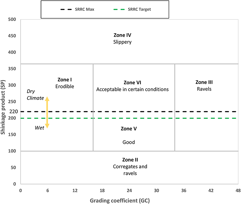
Figure 4. Modified “shrinkage product, grading coefficient performance of base/wearing course” relationship.
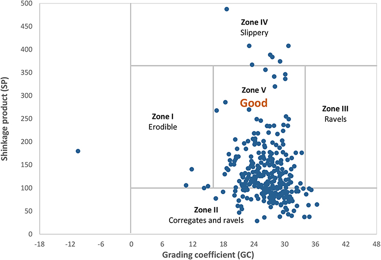
Figure 5. Relationship between shrinkage, grading coefficient, and performance of base/wearing course for gravel [source: Jones and Paige-Green (1996) and Giummarra (2009)].
Gravel loss monitoring stations are established across the region to monitor and compare gravel loss. Figure 6 is a photo of a typical GL monitoring station installed adjacent to a road section. This station is used to record levels over period of time. The permanent control mark was established by driving 1.8 m star picket deep into the ground. Two-star pickets were driven on both sides of the road. Precast concrete surround was placed to make the top surface even with surrounding ground level. Due to safety reasons, a plastic cap was placed on the concrete surface.
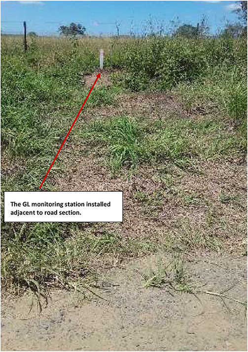
Figure 6. A typical GL monitoring station used on the field.
Twenty road stations with existing material (EM) plus modified material (MM) were compared with 10 stations of EM to compare gravel loss across a section of road. For all stations, ADT varies from 80 to 1,000 and MMP is varied from 50 to 117 mm. Material property noted as PF is the product of plasticity index and material passing through a 26.5 mm sieve. PF of new material varied from 56 to 268. The new material used is as per modified specification and referred to as modified material discussed.
Figure 7 presents the variation in gravel loss (GL) in mm over a number of days (t). On the existing gravel material road sections, the gravel loss was at a higher rate for a shorter duration. For a fair comparison, GL at each station is converted for 365 days (1 year) by extrapolating the recorded gravel loss over specific measured days. On EM, maximum gravel loss was 214.13 mm. The minimum gravel loss was 7.64 mm within 239 days on one location, which is an exception. On the new gravel material road section, the GL was at a lower rate than old gravel and for a longer duration. The maximum GL was 44.37 mm during 365 days and even a marginal GL of 1 mm was recorded over 230 days. The median value of GL is 48.66 mm on EM for 1 year and 7.93 mm on MM.
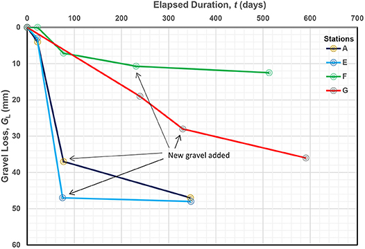
Figure 7. Gravel loss comparison between existing and modified material.
The GL rate is significantly high for old material, which is not modified material. However, no significant maintenance was required for the improved gravel road. There was a lesser need for regrading the roads due to this improved gravel road due to the use of modified gravel material. The field crew confirmed that a gravel road with improved material performed well. Generally, these roads need to be graded within 1 year. Due to the modified material, there is no need to grade for almost 18 months. This demonstrates the benefits of good gravel material. The modified material as per Figure 7 shows consistent results of reduced GL.
There is a huge potential for cost savings by reducing gravel loss on unsealed roads. The majority of the gravel loss rate is between 6 and 10 mm per year. Many studies conclude difficulty predicting deterioration models very accurately for unsealed roads due to a number of variables involved and the requirements of time and resources. Even though some of the models have predicted gravel loss, there is a need to develop a gravel loss model suitable for local conditions.
In this study, a number of gravel loss monitoring stations are established and actual gravel loss is measured. Actual measured gravel loss is compared with the predicted gravel loss from existing models. Based on the field data, the following specific conclusions could be drawn:
a) The current models are not able to capture gravel loss accurately and further data are needed to calibrate parameters resembling localized conditions. While completing the resheeting and re-graveling, the gravel material specification is amended and improved.
b) It is evident that the gravel loss is reduced due to the use of gravel material as per the revised specification. The outcome is reduced gravel loss by the use of this improved material.
c) The soak performance indicator is proposed for revised gravel specification. The revised material is currently being trialed for assessing effectiveness under wet and dry weather conditions.
The datasets generated for this study are available on request to the corresponding author.
VP prepared the draft. SN and HK edited the manuscript.
The authors declare that the research was conducted in the absence of any commercial or financial relationships that could be construed as a potential conflict of interest.
The authors would like to acknowledge Chris Gray, General Manager, Infrastructure Services from the Scenic Rim Regional Council, for providing support for this research project.
Alzubaidi, H., and Rolf, M. (2002). Deterioration and rating of gravel roads: state of the art. Road Mater. Pavement Des. 3, 235–260. doi: 10.1080/14680629.2002.9689924
Bannour, A., Mohamed, E. O., Khadir, E. L., Mohamed, A., Ahmed, B., and Pierre, J. (2019). Optimization of the maintenance strategies of roads in Morocco: calibration study of the degradations models of the highway development and management (HDM-4) for flexible pavements. Int. J. Pavement Eng. 20, 245–254. doi: 10.1080/10298436.2017.1293261
Cocks, G., Ross, K., Colin, L., Paul, F. W. M. L., Tom, B. W. M. L., Andrew, C., et al. (2015). The use of naturally occurring materials for pavements in Western Australia. Aust. Gomech. J. 50, 43–106.
de Percy, M. (2018). Road pricing and road provision in Australia: where are we and how did we get here? Road Pricing and Prov. 11:11–44. doi: 10.22459/RPP.07.2018.02
Ellis, R., and Andrews, B. (2013). “Protocol for the selection of unsealed road material for regional local government,” in International Public Works Conference (Darwin, NT).
Giummarra, G. (2009). Unsealed Roads Manual: Guidelines to Good Practice, 2009 Edn. Melbourne, VIC: Australian Road Research Board.
Giummarra, G. J., Martin, T., Hoque, Z., and Roper, R. (2007). Establishing deterioration models for local roads in Australia. Transp. Res. Record 1989, 270–276. doi: 10.3141/1989-73
Henning, T. F. P. (2015). Unsealed Roads Tactical Asset Management Guide. Road Infrastructure Management Support (RIMS), New Zealand: RIMS.
Henning, T. F. P., Giummarra, G. J., and Roux, D. C. (2008). The Development of Gravel Deterioration Models for Adoption in a New Zealand Gravel Road Management System. Wellington: Land Transport New Zealand.
Henning, T. F. P., Glenn, F., Costello, S. B., Jones, V., and Rodenburg, B. (2015). “Managing gravel-roads on the basis of fundamental material properties,” in Transportation Research Board 94th Annual Meeting (Washington, DC).
Jones, D., and Paige-Green, P. (1996). “The development of performance related material specifications and the role of dust palliatives in the upgrading of unpaved roads,” in Combined 18th ARRB Transport Research Conference and Transit New Zealand Land Transport Symposium (Christchurch).
Linard, K. (2010). “A system dynamics modelling approach to gravel road maintenance management,” in 24th ARRB Conference (Melbourne, VIC).
Martin, T., Choummanivong, L., Thoresen, T., Toole, T., and Kadar, P. (2013). “Deterioration and maintenance of local roads,” in International Public Works Conference (Darwin, NT).
McManus, K. J. (1994). “Pavement deterioration models for a local government authority,” in 17TH ARRB Conference, Gold Coast (Beaudesert, QLD).
Mwaipungu, R. R. (2015). The Formulation and Application of a Gravel Loss Model in Management of Gravel Roads in Iringa Region, Tanzania. Ph.D. thesis, Durban University of Technology, Durban, South Africa.
Mwaipungu, R. R., and Allopi, D. (2014). The sustainability of gravel roads as depicted by sub Saharan Africa's standard specifications and manuals for road works: Tanzania case study. WIT Trans. Built Environ. 138:581–592. doi: 10.2495/UT140481
Paige-Green, P. (1989). The Influence of the Geological and Geotechnical Properties on the Performance of Materials for Gravel Roads. Ph.D. thesis, University of Pretoria, Pretoria, South Africa.
Paige-Green, P. (2007). Local Government Note: New Perspectives of Unsealed Roads in South Africa. Melbourne, VIC: ARRB Group.
Paterson, W. (1991). Deterioration and maintenance of unpaved roads: models of roughness and material loss. Transport. Res. Record 1291, 143–156.
Scenic Rim Regional Council (SRRC) (2018). 2018-19 Community Budget Report Scenic Rim Regional Council. Beaudesert, QLD: Scenic Rim Regional Council.
Tim, M., and Choummanivong, L. (2016). The benefits of Long-Term Pavement Performance (LTPP) research to funders. Transport. Res. Proc. 14, 2477–2486. doi: 10.1016/j.trpro.2016.05.311
Uys, R. (2011). Evaluation of gravel loss deterioration models: case study. Transport. Res. Record 2205, 86–94. doi: 10.3141/2205-12
Keywords: gravel loss, gradation, prediction model, modified gravel, unsealed road
Citation: Pardeshi V, Nimbalkar S and Khabbaz H (2020) Field Assessment of Gravel Loss on Unsealed Roads in Australia. Front. Built Environ. 6:3. doi: 10.3389/fbuil.2020.00003
Received: 26 October 2019; Accepted: 10 January 2020;
Published: 13 February 2020.
Edited by:
Sakdirat Kaewunruen, University of Birmingham, United KingdomCopyright © 2020 Pardeshi, Nimbalkar and Khabbaz. This is an open-access article distributed under the terms of the Creative Commons Attribution License (CC BY). The use, distribution or reproduction in other forums is permitted, provided the original author(s) and the copyright owner(s) are credited and that the original publication in this journal is cited, in accordance with accepted academic practice. No use, distribution or reproduction is permitted which does not comply with these terms.
*Correspondence: Vasantsingh Pardeshi, dmFzYW50c2luZ2hiaGltc2luZ2gucGFyZGVzaGlAc3R1ZGVudC51dHMuZWR1LmF1
Disclaimer: All claims expressed in this article are solely those of the authors and do not necessarily represent those of their affiliated organizations, or those of the publisher, the editors and the reviewers. Any product that may be evaluated in this article or claim that may be made by its manufacturer is not guaranteed or endorsed by the publisher.
Research integrity at Frontiers
Learn more about the work of our research integrity team to safeguard the quality of each article we publish.