 Arka P. Reksowardojo
 Gennaro Senatore
 Ian F. C. Smith
94% of researchers rate our articles as excellent or good
Learn more about the work of our research integrity team to safeguard the quality of each article we publish.
Find out more
ORIGINAL RESEARCH article
Front. Built Environ. , 10 July 2019
Sec. Structural Sensing, Control and Asset Management
Volume 5 - 2019 | https://doi.org/10.3389/fbuil.2019.00093
This article is part of the Research Topic Design and Control of Adaptive Civil Structures View all 13 articles
Adaptive structures have the ability to modify their shape and internal forces through sensing and actuation in order to maintain optimal performance under changing actions. Previous studies have shown that substantial whole-life energy savings with respect to traditional passive designs can be achieved through well-conceived adaptive design strategies. The whole-life energy comprises an embodied part in the material and an operational part for structural adaptation. Structural adaptation through controlled large shape changes allows a significant stress redistribution so that the design is not governed by extreme loads with long return periods. This way, material utilization is maximized and embodied energy is reduced. A design process based on shape optimization has been formulated to obtain shapes that are optimal for each load case. A geometrically non-linear force method is employed to control the structure into required shapes. This paper presents the experimental testing of a small-scale prototype adaptive structure produced by this design process. The structure is a simply supported planar truss. Shape adaptation is achieved through controlled length changes of turnbuckles that strategically replace some of the structural elements. The stress is monitored by strain sensors fitted on some of the truss elements. The nodal coordinates are monitored by an optical tracking system. Numerical predictions and measurements have a minimum Pearson correlation of 0.86 which indicates good accordance. Although scaling effects have to be further investigated, experimental testing on a small-scale prototype has been useful to assess the feasibility of the design and control methods outlined in this work. Results show that stress homogenization through controlled large shape changes is feasible.
Civil structures are designed to meet strength and deformation criteria for critical load cases. Since extreme and thus rarely occurring loads have to be accounted for, the structural capacity is not fully utilized for most of the service life of the structure. The construction sector, however, is a major contributor to the global energy demand (Straube, 2006) as well as a major consumer of raw materials (United Nations Environmental Programme, 2007), and therefore it is of growing importance to minimize environmental impacts of load-bearing structures.
Structural adaptation through sensing and actuation is a potential solution. If the structure is able to counteract the effect of loads through active control, it can be designed to maintain optimal performance as the external load changes (Yao, 1972; Soong, 1988). The potential of structural adaptation as a means to mitigate the dynamic response during the occurrence of extreme loads (e.g., earthquakes, strong winds) has been subject of extensive research (Skelton et al., 1992; Reinhorn et al., 1993; Soong and Cimellaro, 2009). More recently, the potential of using adaptation to design structures with a better material utilization has been investigated (Sobek and Teuffel, 2001; Cimellaro et al., 2008). A new design criterion for adaptive structures has been introduced in Senatore et al. (2019), which is “whole-life” energy comprising a part embodied in the material and another part for control and adaptation. It was shown that substantial whole-life energy savings can be achieved through adaptive design strategies (Senatore et al., 2018). Instead of relying solely on passive resistance provided by material and form, strategically located actuators change the internal forces and shape of the structure to ensure safety and serviceability. Since actuation is only employed for rarely occurring loading, reduction in material embodied energy can be achieved with a small increase in control operational energy as a trade-off. It was shown that whole-life energy savings as high as 70% can be achieved through this design strategy (Senatore et al., 2018a,b).
Shape optimization is usually employed to optimize the geometry of structures under worst load cases (Gil and Andreu, 2000; Wang et al., 2002; Shea and Smith, 2006). When applied to reticular structures, the optimization process can lead to large modifications of nodal coordinates starting from an initial layout, to an extent that the internal forces are manipulated significantly (Descamps and Coelho, 2013). Through this process, shapes resembling arches, catenaries, and lenticular configurations have been found to be efficient in terms of material utilization (Gil and Andreu, 2000). Using a similar approach (Pedersen and Nielsen, 2003), it was shown that small but strategic adjustments of the shape result in weight savings up to 35% without changing the main geometric features. However, the geometry obtained through these methods is fixed and thus, the structural capacity is only partially utilized under peak demands.
Shape control involving large shape changes has been studied numerically and experimentally for deployable and tensegrity structures (Tibert, 2002; Fest et al., 2003; Veuve et al., 2015). In this context, large shape changes have been achieved through mechanisms. However, the use of mechanisms based on moving parts often results in a significant penalty due to the weight of the joints and increased control complexity (Campanile, 2003). Shape control through flexibility has received little attention both theoretically and experimentally. Shape and force control of a reticular adaptive structure has been successfully tested in Senatore et al. (2018); however, geometric non-linearity was not accounted for. Formulations of geometrically non-linear shape and force control exist (Yuan et al., 2016), nonetheless experimental validation is still lacking.
Recent work has investigated the efficacy of structural adaptation through large shape changes (Reksowardojo et al., 2018). Numerical studies have shown that a substantial amount of embodied energy can be saved with respect to structures that are able to adapt through small shape changes. Through large geometry reconfiguration, the internal forces can be redistributed effectively and thus, the design is not governed by extreme loading. This paper presents details of the experimental testing of a small-scale prototype adaptive structure produced by the methods presented in Reksowardojo et al. (2018). The prototype tested in this work is a simply-supported planar-truss beam. Shape adaptation is achieved through controlled length changes of turnbuckles that strategically replace some of the structural elements. Strain sensors and an optical tracking system are employed to monitor element stress and nodal displacements. The aim of this work is to validate experimentally the feasibility of shape and force control through the process outlined in Reksowardojo et al. (2018) on a small-scale prototype. Results from this test will inform future research on larger scale adaptive structures.
The design method consists of two parts: (1) optimization of the geometry, internal forces and element cross-section areas to minimize the structure embodied energy, (2) optimal actuator placement to control the structure into the optimal shapes obtained in (1) through quasi-static, non-linear geometric shape and force control. The design process is illustrated in Figure 1. The design method is formulated for reticular structures and this study only deals with such structures. The actuators are assumed to be linear actuators integrated into the structure by replacing selected elements. This design method has been formulated for structures subjected to slowly changing loads (e.g., snow load). The control methods adopted in this formulation are for quasi-static or low frequency loading hence the dynamic response of the structure is not taken into account.
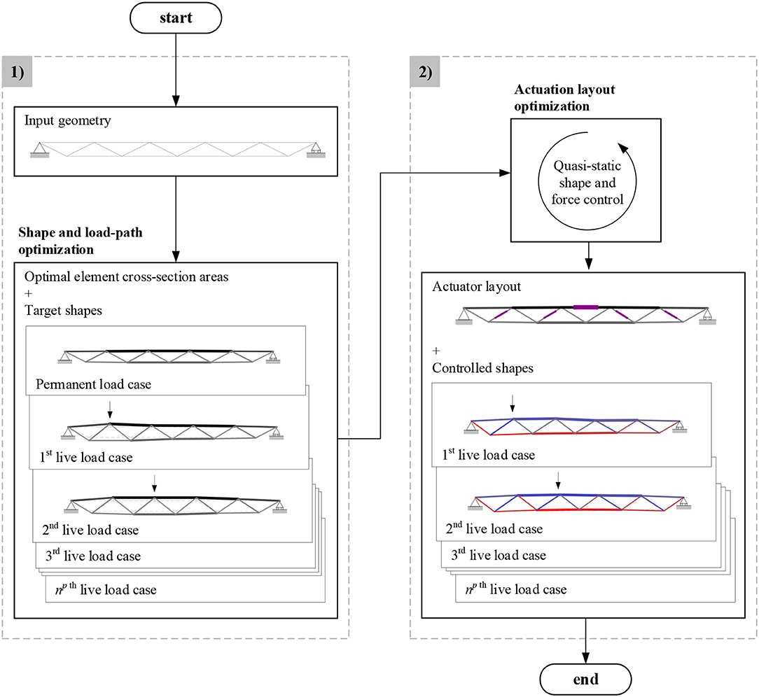
Figure 1. Design method flowchart.
The structure is designed to have an optimal shape and an optimal internal load path against each load case. This process, denoted by χ, is a mapping between external load p and target shapes dt as well as internal forces ft that are optimized to maximize material utilization:
The superscript t stands for “target.” The inputs are the structural topology, i.e., a set of nn nodes connected by ne elements, support conditions, loading and controlled degrees of freedom ncd. The controlled degrees of freedom identify the nodal positions that will be varied during shape optimization and that will be controlled through actuation. The initial shape of the structure (i.e., initial node coordinates) is defined as dinput ∈ ℝnd. The design variables are element cross-section areas α ∈ ℝne, internal forces ft ∈ ℝne and nodal positions dt ∈ ℝnd:
The objective is to minimize the embodied energy of the structure subject to force equilibrium and stress constraints including element buckling:
The index i refers to the ith element, j to the jth load case, ne is the number of elements and np is the total number of load cases. In Equation (2) gi is the material energy intensity (Hammond and Jones, 2008) and ρi the density of the ith element. The term lij is the length of the ith element for the jth load case. The second moment of area Ii, is a function of the cross-section area αi. E, σt and σc are the Young's modulus, admissible tensile and compressive stress respectively. , and pj are the equilibrium matrix, internal forces and external load for the jth load case. Upper and lower bounds are set in order to avoid potential convergence issues caused by node position reversal or merging as well as to ensure control feasibility. The output of this process includes the element cross-section areas α as well as the optimal forces and nodal positions for each load case.
At this stage, geometric compatibility between element deformations and nodal displacements is not accounted for and thus, the resulting target shapes may not be compatible. Geometric compatibility is a non-linear constraint which can cause convergence difficulties and hence, it is often ignored in structural optimization. For a passive structure, the omission of this constraint might result in a configuration that does not meet serviceability limits (e.g., deflection) under loading. For adaptive structures, disaggregation of force equilibrium and geometric compatibility is a key aspect (Senatore et al., 2019). Geometric compatibility is instead enforced through a controlled shape change. This way, a structure can be designed to meet strength requirements passively but serviceability constraints are met through adaptation i.e., shape and internal force control.
The second step of the design process is to obtain an actuator layout (i.e., placement) that is optimal to control the structure into the target shapes obtained in section Shape and Load-Path Optimization. The objective is to maximize the similarity between shapes controlled via actuation Δdc and the target shapes obtained in section Shape and Load-Path Optimization subject to ultimate limit state (ULS) constraints:
where:
Δdt is the nodal displacement vector to move from the deformed shape to the target shape dt. Δdc is the nodal displacement vector to move from the deformed shape to the shape obtained through control (section Quasi-Static, Non-linear Geometric Shape, and Force Control). Both equilibrium and geometric compatibility must be considered at this stage. The design variable y ∈ ℤnact is a vector containing the indices of the active elements and nact is the number of actuators. Q is a similarity criterion (Tanimoto, 1958) which is employed in this work to measure the difference between two vectors in terms of shape features and node positions. The index Q takes a value between 0 and 1.
The optimization stated in Equations (8)–(10) is combinatorial and thus, when the number of structural elements is large a full enumeration is impossible. Optimal actuator placement is carried out using a global search method called constrained simulated annealing (CSA) (Wah and Wang, 1999). A heuristic based on a measure of efficacy for each element to contribute toward the attainment of the optimal shapes through its length changes (Senatore et al., 2019) is employed to generate the initial candidate solution and to define the neighborhood structure i.e., the set of feasible solutions “close” to the current solution.
The structure has to be controlled through actuator commands Δlthat cause a change of internal forces Δfc and nodal displacement Δdc that approximate the target ones (Δft, Δdt):
Since large shape changes modify equilibrium conditions, control commands must be computed through a method that considers geometric non-linearity. In addition, because shape adaptation does not rely on mechanisms with defined kinematics, given an actuator layout there are generally infinite solutions in terms of length changes to approximate a required shape change. A possible strategy is to find the minimum actuator length changes that deform the structure into a target shape. This is an inverse problem having a non-trivial solution.
For small deformations, the relationship between element length changes Δl to shape changes Δd and internal force changes Δf can be expressed as:
where Sf and Sd are the force and displacement sensitivity matrices (Senatore et al., 2019). In this work, Sf and Sd are computed using a force method based on singular value decomposition of the equilibrium matrix (Pellegrino, 1993; Luo and Lu, 2006; Yuan et al., 2016). Once the force and displacement sensitivity matrices are known, ϕ−1 is formulated as a constrained minimization of the difference between the controlled (Δdc, Δfc) and optimal configuration (Δdt, Δft):
where the term S is:
When geometrical non-linearity is accounted for, Sd and Sf have to be updated as the geometry of the structure changes. The Newton-Raphson scheme is employed to iterate to convergence which is reached when the change of forces ‖Δfc − Δfc′‖2 and displacements ‖Δdc − Δdc′‖2 between two consecutive iterations are smaller than a set tolerance, where Δfc′ and Δdc′ are the change of forces and shape at next iteration.
The prototype structure tested in this study is a planar simply-supported truss which can be thought of as a part of the roof system shown in Figure 2A. The truss has a span of 1,000 mm and a 20:1 span-to-depth ratio. It consists of 19 elements connected through 11 nodes of which two are constrained as indicated in the diagram shown in Figure 2B. The truss is statically determinate. All elements have a solid cylindrical section and are made of aluminum with a Young's modulus of 72.4 GPa.
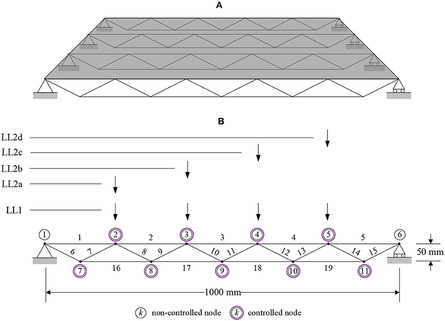
Figure 2. Description of the case study. (A) Roof structure case study. (B) Loading, node and element numberings.
Due to the small scale of this structure its self-weight is negligible. Two live loads (LL) are considered: (1) a uniformly distributed load of 10 N applied on all top chord nodes (LL1); (2) a moving load discretized by four point loads of 20 N applied on each node of the top chord in turn (LL2a−2L2d).
All nodes except the supports are allowed to shift vertically with an upper bound Δdu and a lower bound Δdl set to ±15 mm. The lower bound for the element radius is set to 1 mm. The first step of the method outlined in section Shape and Load-Path Optimization produces a structure whose embodied energy is reduced by 17% with respect to an identical weight-optimized passive structure.
A low number of actuators is generally preferred in order to reduce monetary cost and control complexity. A minimum number of actuators is determined by applying sequentially the actuator layout optimization process (section Actuation Layout Optimization), each time decreasing the number of actuators until no solution can be obtained that satisfies ULS requirements. Figure 3 shows the layouts obtained for 19, 14, 10, 7, 5, and 4 actuators.
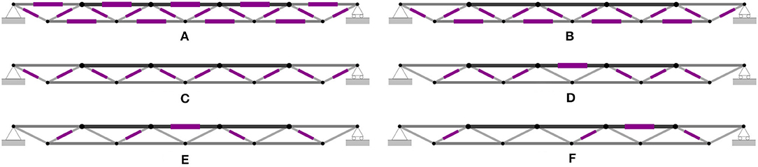
Figure 3. Optimal actuator layouts for 19, 14, 10, 7, 5, and 4 active elements. (A) 19 actuators (all elements), (B) 14 actuators, (C) 10 actuators, (D) 7 actuators, (E) 5 actuators, and (F) 4 actuators, not feasible.
No feasible solution (ULS satisfied) can be found for layouts made of less than 5 actuators. The layout shown in Figure 3F is an infeasible solution for 4 actuators. With this layout, the maximum element demand/capacity ratio is 1.26. With 5 actuators the maximum element demand/capacity ratio of 0.83. The 5-actuator solution is therefore chosen as the optimal actuator layout (Figure 3E). This solution was obtained after 413 iterations in 651 s on an Intel Core i7, 3.60 GHz. This layout has been verified through a full enumeration (11,628 candidate solutions) which has taken ~5 h.
The target shapes are shown in Figure 4A. For comparison, Figure 4B shows the controlled shapes (5-actuator layout) with the element stress mapped onto the geometry. Optimal shapes and controlled shapes are very similar but not identical. There is a maximum distance of 11.8 mm for node 8 between target and controlled shape under LL2b. Table 1 gives the actuator length changes for all load cases.

Figure 4. Target (A) and controlled (B) shapes.
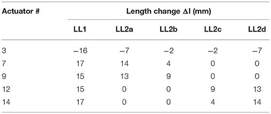
Table 1. Actuator length changes.
In order to show stress redistribution through active control, the adaptive solution is compared to an identical weight-optimized passive structure. In this context, stress homogenization is understood as a reduction of magnitude and variability. For example, it is clear from Figure 4 that through shape control the depth of the structure increases in the proximity of the point of application of the external load. If the structure is thought of as a beam, this results in a better resistance against bending moment.
Figure 5 shows the element stress for the passive (a) and adaptive (b) structures. For brevity, LL2c and LL2d are not shown since they are mirror of LL2b and LL2a. Tensile and compressive stress are indicated in red and blue, respectively. The mean for each data set is shown as a horizontal dashed line. Stress variability is quantified through standard deviation. The width of the shaded band, whose centerline is the mean value of each data set, is twice the standard deviation.
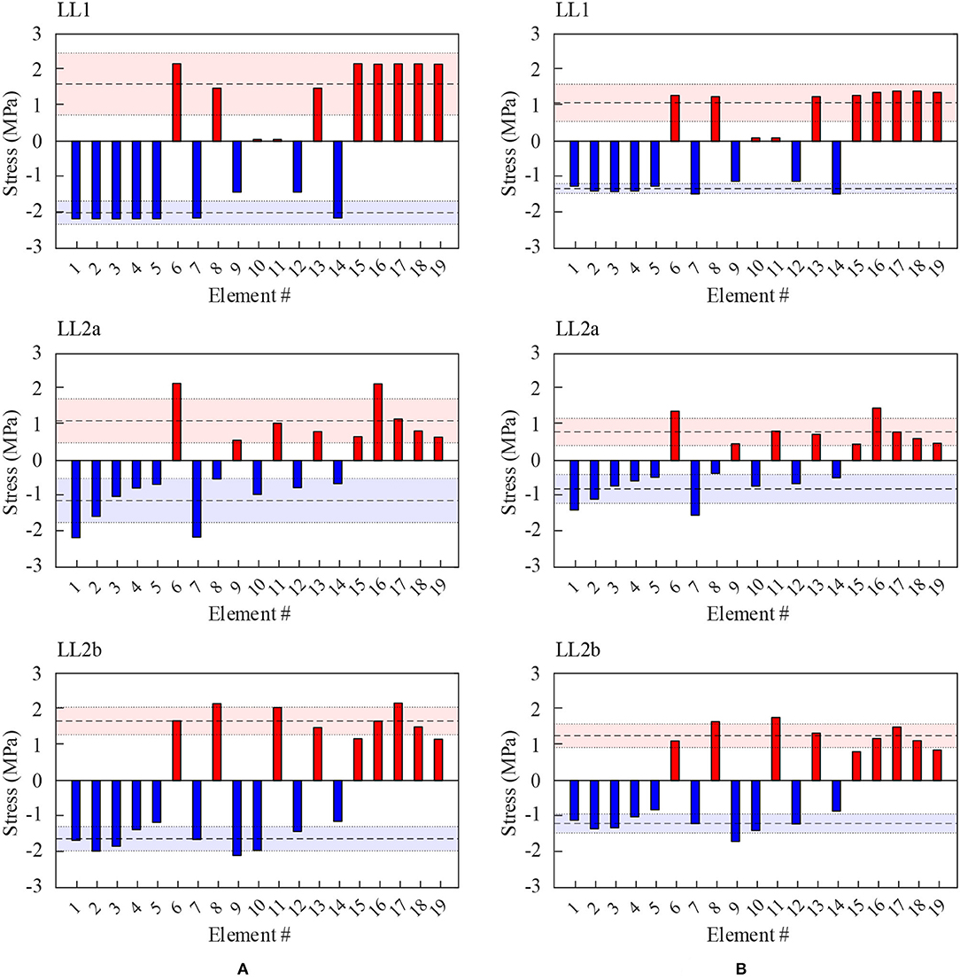
Figure 5. Element stress in passive (A) and adaptive (B) structure.
The element stress in the adaptive structure is consistently lower than that of the passive structure. The maximum mean reduction for tensile and compressive stress are 33 and 34%, respectively (both in LL1). The same applies to stress variability. LL1 and LL2b have the smallest variability through shape control for compressive and tensile stress, respectively. Stress homogenization can be appreciated the most in LL1. The stress of element 8, 9, 12, and 13 remains similar to that of the corresponding elements in the passive structure. However, the stress of element 1 ~ 7 and 14 ~ 19 decrease. Similarly, in LL2a, the stress of element 6, 7, and 16 decrease significantly while the stress for the other elements remain practically the same. There is no stress reversal between the passive and adaptive structure.
The aim of this test is to assess the applicability of the design method outlined in section Shape and Load-Path Optimization and Actuation Layout Optimization to a real structure, as well as the accuracy of the numerical methods for shape control outlined in section Quasi-Static, Non-linear Geometric Shape, and Force Control. A prototype structure was built based on the model described in section Numerical Case Study. Figure 6 shows a bar chart comparing the cross section area between the passive and adaptive structure obtained through simulation with the built prototype. Assuming the density of aluminum is 2,649 kg/m3, the mass of the passive and adaptive structure is 0.35 and 0.28 kg, respectively. The element cross sections of the built prototype have been sized-up to match commercial availability. The total mass of the prototype is 0.32 kg, of which the mass of the actuators comprises 1%.
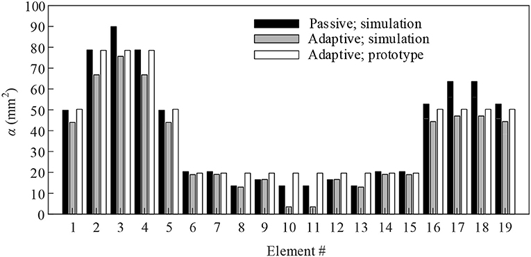
Figure 6. Optimal cross-section sizing.
The active elements are five turnbuckles that are fitted on element 3, 7, 9, 12, and 14 according to the 5-actuator layout obtained in section Numerical Case Study. Each turnbuckle consists of a shaft hosting two rods of opposite threads (left and right). This way, rotating the shaft can either shorten or lengthen the turnbuckle (i.e., contraction or extension) depending on the rotation direction.
The joints are fabricated through additive manufacturing using a polymer-based material (polyether block amide) with a Young's modulus of 82 MPa. The low stiffness of this material was chosen to ease shape reconfiguration, which in this case is manually operated through the turnbuckles. Due to the planarity of the truss, to avoid out-of-plane deflections, two acrylic posts are placed at 300 mm from both ends as shown in Figure 7A. These posts are in direct contact with the structure allowing only in-plane movements. Although not shown in Figure 7A, the right support can slide horizontally through a pin-slot joint.
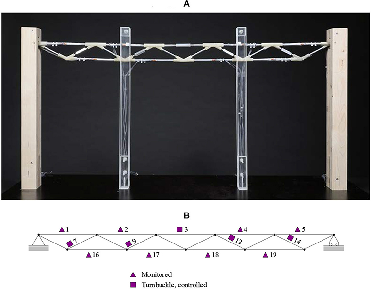
Figure 7. Experimental setup. (A) Structure and supports. (B) Location of sensors and turnbuckles.
Elements 1, 2, 4, 5, 16, 17, 18, and 19 are instrumented with strain sensors. Only 8 out of 19 elements are instrumented because it was not practical to install strain gauges on the 5 mm diameter bracing elements and on the turnbuckles. Figure 7B shows the location of both actuators and strain sensors. Figure 8 is a close-up taken at mid-span showing some of the turnbuckles and strain sensors.
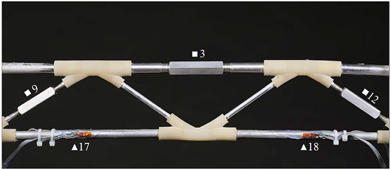
Figure 8. Sensors and turnbuckles fitted in the truss.
For each element, two strain gauges are placed diametrically opposed to one another in a quarter-bridge configuration. The strain of the ith element is computed as where and are the strains measured at each gauge position. By doing so, flexural effects are rejected, since strains of opposing signs cancel each other. To reduce the effect of out-of-plane actions, the gauges are placed parallel to the truss main plane. The strain gauges used in this test have a resistance of 350 Ω ± 0.35% and a gauge factor of 2.06 ± 1.0%. The gauges are manufactured by Hottinger Baldwin Messtechnik (HBM).
The node position is monitored using an optical tracking system by OptiTrack comprising four cameras and reflective targets that are placed on the nodes. The optical system is able to track the node position within a ±0.025 mm precision. Data acquisition of strains and nodal positions was carried out with a sampling rate of 10 Hz using National Instruments PXIe-8840 with Intel Core i7, 2.60 GHz quad-core. Loading consists of weights of 1 kg (≈10 N) and 2 kg (≈20 N) for LL1 and LL2, respectively which are applied on the nodes using hooks.
The structure static response under loading is measured and compared to the numerical predictions obtained in section Numerical Case Study. Element strains and nodal positions are measured before and after shape control. Figure 9 shows the difference between Δdcm and Δdcs (measured and simulated controlled shape changes) represented by thick and dashed lines respectively (Figure 4B). Referring to the similarity criterion given in Equation (10), a similarity of 0.78 is obtained between Δdcs and Δdcm. Table 2A gives the maximum Euclidean distance between the nodes of Δdcs and Δdcm (measured and simulated controlled shapes) as well as the norm of the difference between Δdcs and Δdcm. There was a maximum of 12.2 mm for node 8 between Δdcs and Δdcm under LL2b.
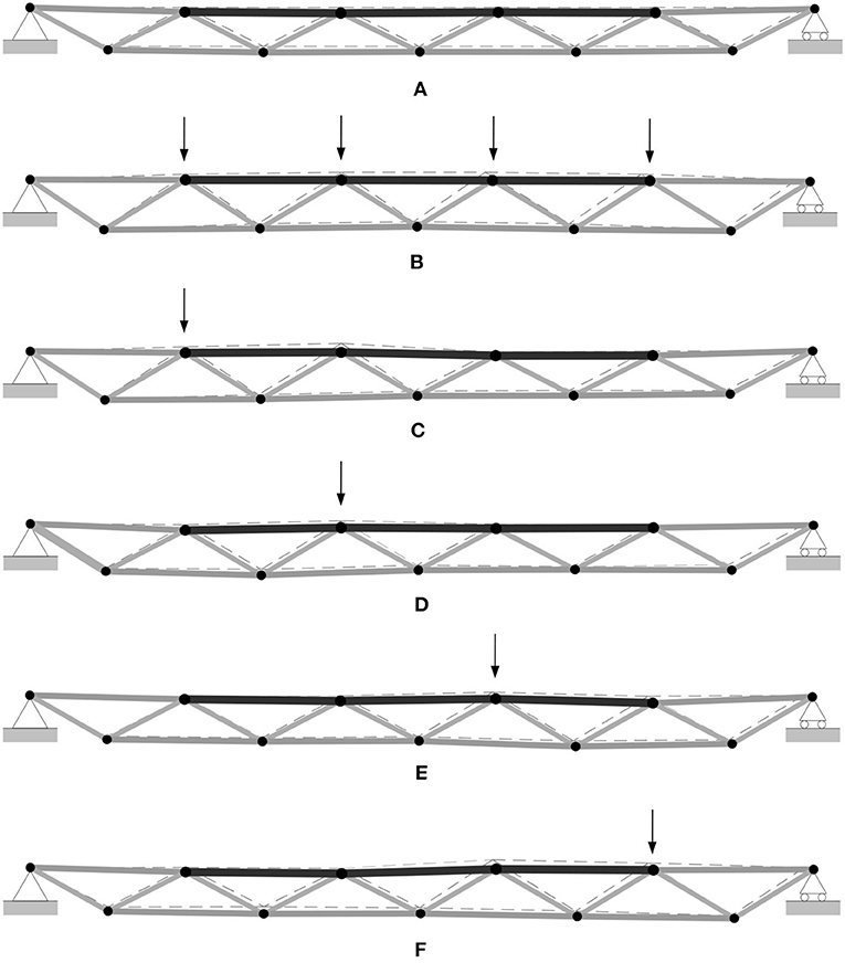
Figure 9. Controlled shapes: measurement (thick lines) vs. simulation (dashed lines). (A) No load, (B) LL1, (C) LL2a, (D) LL2b, (E) LL2c, and (F) LL2d.
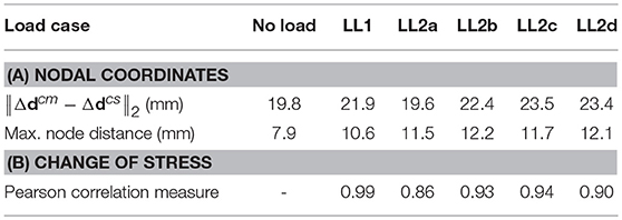
Table 2. Discrepancy between measurement and simulation.
The measured structure response under shape control is consistent with the numerical predictions (section Numerical Case Study); an overall reduction of tensile and compressive stress is observed. This reduction is caused by the increase in depth in proximity of the point of application of the external load. The bar charts in Figure 10 compare element stresses obtained from simulation and the measured ones for all load cases. For brevity, LL2c and LL2d are not shown since they mirror LL2b and LL2a, respectively. The element stress predicted by simulations before and after control is shown in white and gray respectively. The element stress measured before and after control is indicated by hatching.
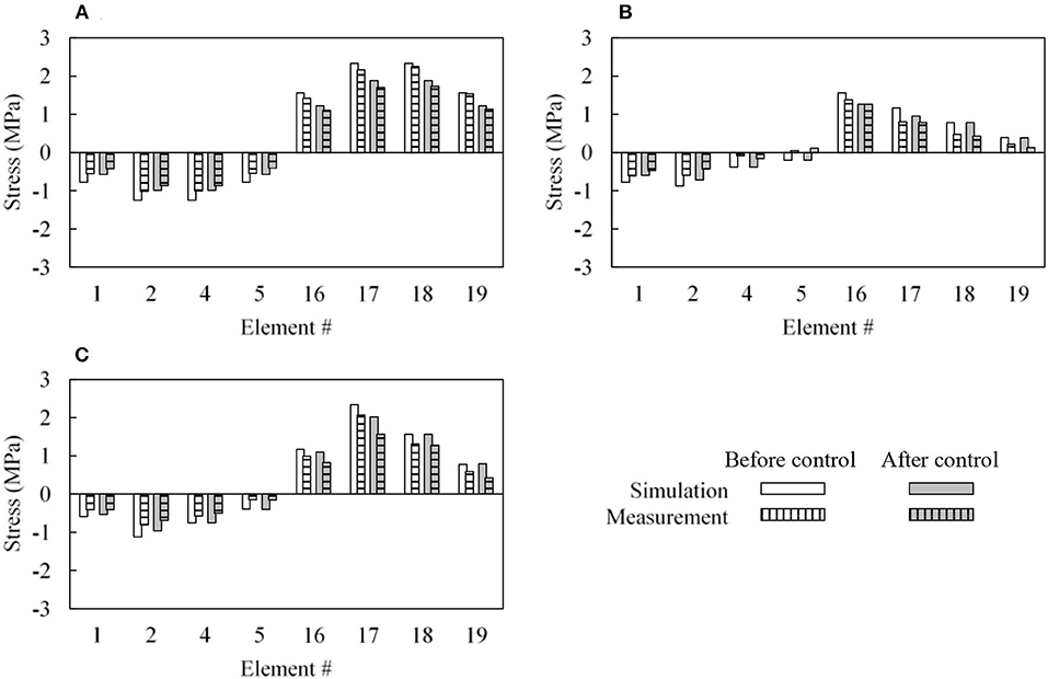
Figure 10. Element stress. (A) LL1, (B) LL2a, and (C) LL2b.
Table 2B shows the Pearson correlation (Hollander and Wolfe, 1973) between measured and predicted change of stress (the change of stress before and after control). A strong correlation between measurement and prediction is obtained for all load cases.
Tables 3A,B give metrics related to predicted and measured element stress distribution respectively. When assessing the effect of shape control (i.e., stress reduction and homogenization) predicted through simulations in Simulated vs. Measured Controlled Shapes (Figure 5), it was observed that both mean and standard deviation of the element stress are lower in the adaptive compared to the weight-optimized passive structure. Generally, this is also observed through measurement. The mean of the stress is lower for all load cases. The maximum mean reduction for tensile and compressive stress are 25% (LL1) and 32% (LL2d), respectively. However, the standard deviations for compressive stress for LL1, LL2a, and LL2d is higher for the adaptive structure because the element cross sections had to be changed due to commercial availability. The symbol “▴” in Table 3 indicates cases where mean or standard deviation of the element stress in the adaptive structure is higher than in the weight-optimized passive structure.
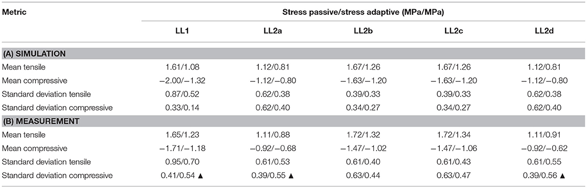
Table 3. Element stress passive vs. adaptive structure.
To implement a control system based on the optimization process outlined in section Shape and Load-Path Optimization, the external load p has to be sensed in order to compute the target shapes dt. When the internal forces and the shape of the structure are known, the external loads p can be inferred through force equilibrium:
where A is the equilibrium matrix which is iteratively updated based on the measured nodal positions, f is the vector of internal forces obtained directly through strain measurement. Because the structure undergoes a large shape change, the equilibrium matrix A cannot be kept constant. For example, if A is not updated as the shape changes, the sensed external load p may appear to vary even if it is kept constant.
Since only 8 out of 19 elements are instrumented with strain gauges, the forces in non-instrumented elements are obtained through nodal equilibrium. Force equilibrium can be expressed as a homogeneous linear system for a node whose degree of freedoms are not constrained (i.e., it is not a support) and when no external load is applied on it:
Node 7, 8, 9, 10, and 11 satisfy these criteria (Figure 2B), therefore the forces in elements 6 to 15 can be computed through Equation (18). It is not possible to compute the force in element 3 using Equation (18) because it connects node 3 and 4 where the external load is applied. In this case, force equilibrium is an underdetermined linear system with more unknowns than equations. Therefore, the force in element 3 is inferred through linear regression. The input dataset is obtained through simulation, the known values of f are the independent variables. Load cases LL1 and LL2 were investigated.
Figure 11A shows the comparison between applied (continuous) and predicted (scatter) external load on node 2 (load case LL2a) when no shape control was carried out. A 20 N load was applied incrementally in four steps of 5 N. Load prediction was carried out 10 times per second. The external load predicted for node 2 was in good agreement with the applied one, with a maximum error of 1.1 N when the load magnitude reaches 20 N. Despite no load was applied on node 3, 4, and 5, spurious vertical loads of 1.8 N magnitude were predicted.
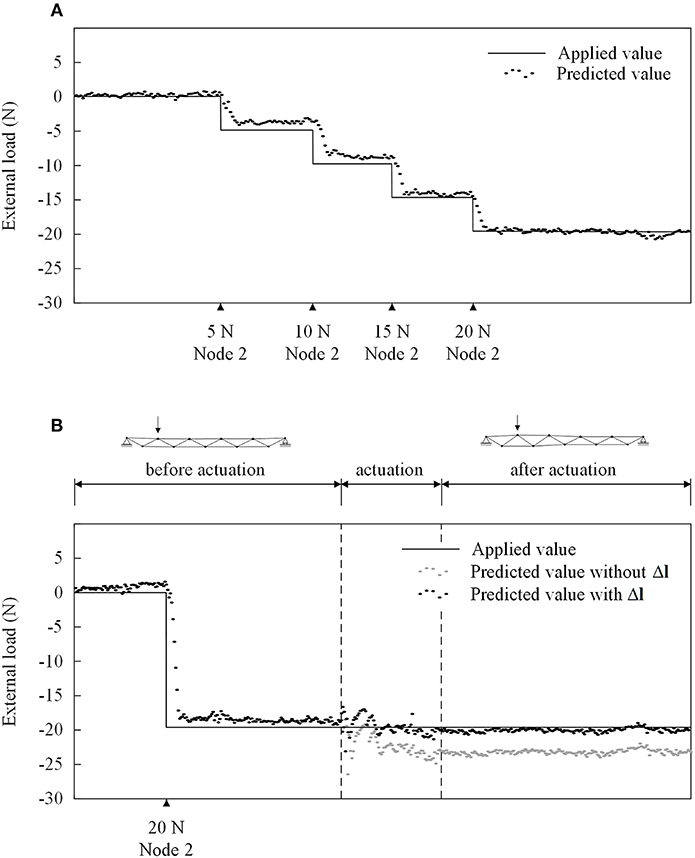
Figure 11. External load on node 2 (load case LL2a). (A) No shape control. (B) Shape control.
Figure 11B shows the comparison between applied and predicted values for the external load when the structure is subjected to a 20 N load (applied in one step) on node 2 before and after control. Shape control was carried out by applying the length changes Δl for load case LL2a. By using a linear regression model that considers only the known values of f as the independent variables, prediction of the external load p had a maximum error of 4 N as shown by the gray scatter plot in Figure 11B. Load prediction was more accurate when the length changes Δl were also included in the independent variables in order to obtain the forces in non-instrumented elements. As shown by the black scatter plot in Figure 11B, the predicted load is close to the applied one even after shape control with a maximum error of 0.6 N. As in the previous case, despite no load was applied on node 3, 4, and 5, spurious vertical loads of 2.3 N magnitude were predicted.
Similarly, for load case LL1, 10 N loads were applied to node 2, 3, 4, and 5 sequentially and when no shape control was carried out. Figure 12A shows the comparison between the applied (continuous) and predicted (scatter) external load. The external load was predicted with good accuracy, with a maximum error of 2 N for node 4. Prediction error varied when adjacent nodes were loaded. For example, the load predicted on node 2 is on average 9.2 N. However, when the load is applied on node 2 and 3 simultaneously the predicted value was 9.7 N.
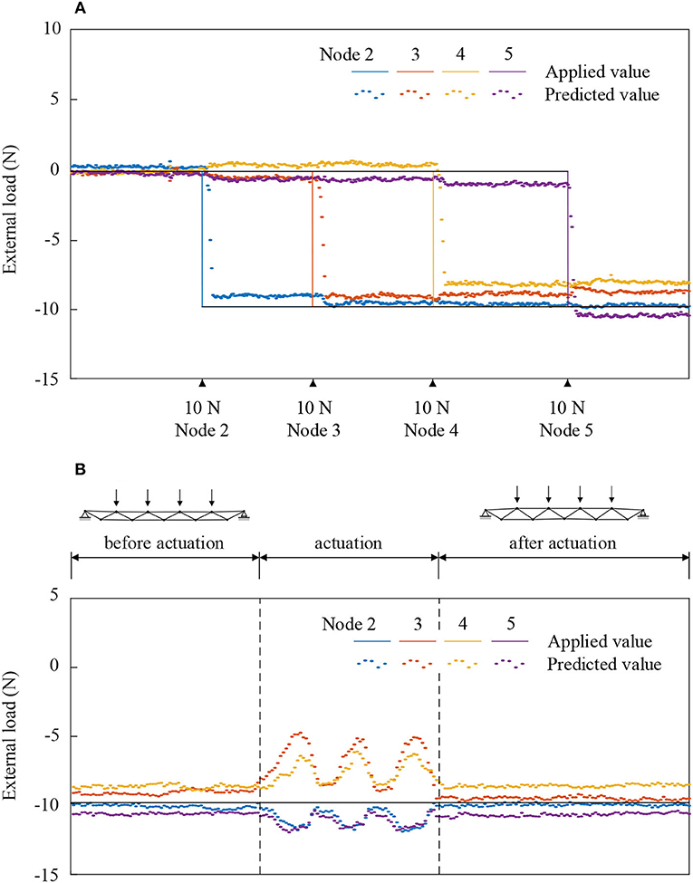
Figure 12. External load on node 2, 4, 6, and 8 (load case LL1). (A) No shape control. (B) Shape control.
When shape control is carried out under LL1, the external load was predicted with good accuracy, with a maximum error of 2.3 N for node 4. Higher prediction errors occurred during actuation, as shown in Figure 12B, which involved manual adjustment of several turnbuckles.
This work has presented experimental testing of a small-scale adaptive planar truss that counteracts loading through controlled large shape changes. This structure was designed using a design method outlined in section Design Method, which involves a shape optimization process, through which an optimal shape is obtained for each load case. This way the design is not governed by peak loads. Stress homogenization through shape control allows a structure to operate closer to design limits maximizing material utilization and thus saving embodied energy with respect to a passive structure.
Stress homogenization has been quantified by comparing the mean and standard deviation of the element stress for the adaptive structure to those of an equivalent weight-optimized passive structure. Although the cross-section of the elements in the adaptive structure are smaller than those in the passive one, both mean and standard deviation of the stress are lower for the adaptive thanks to shape control. The maximum mean reduction for tensile and compressive stress are 25 and 32%, respectively. Experimental results show good agreement with numerical simulations. A minimum Pearson correlation coefficient of 0.86 has been observed. The formulation outlined in this study treats the element cross section area as continuous variables. However, the element cross sections are subject to commercial availability. Future works could look into implementing a similar optimization process by treating the element cross sections as discrete variables using mixed-integer programming.
Shape and force control based on the formulation outlined in this paper requires knowledge of the external load. In this work, the external load was inferred from sparse strain measurements (only 8 elements instrumented out of 19) complemented by an optical tracking system. The optical system was essential to close the information gap caused by sparse instrumentation, especially in situations where nodal coordinates varied through shape control. However, the use of machine vision may pose a reliability risk in practice as the monitoring of nodal coordinates may fail when multiple reflective markers are occluded. Methods that mitigate this failure could be subject of future investigation.
Since experimental testing was carried out at a small scale, the effect of the structure self-weight and that of the actuators is negligible. However, this effect becomes significant with scale, especially due to the weight of the actuators, and thus it is important to include it in optimization and control. An approach proposed in Senatore et al. (2019) is to estimate the weight of an actuator by assuming it is proportional to the required force capacity.
The results of this study lead to the following conclusions:
• Experimental testing on a small-scale prototype has demonstrated that stress homogenization through large-shape changes is feasible. This enables an adaptive structure to operate closer to design limits maximizing material utilization and thus saving embodied energy with respect to a passive structure.
• The geometrically non-linear force method (NFM) outlined in section Quasi-Static, Non-linear Geometric Shape and Force Control offers an efficient way to control the shape of a reticular structure under quasi-static loading as shown by the good accordance between simulation and measurement.
• Detection of the applied loading is necessary for non-linear shape and force control.
It is expected that tests on similar full-scale reticular structures designed using the design method outlined in this work will lead to similar conclusions. Experimental testing at a small scale has allowed model validation without including the effect of node stiffness on internal forces and nodal displacements, as well as how this effect behaves with scale. For this reason, further work will involve testing on a larger scale prototype adaptive structure.
The raw data supporting the conclusions of this manuscript will be made available by the authors, without undue reservation, to any qualified researcher.
GS set up research objectives and directions with contribution from IS. Method implementation were carried out by AR and GS. AR carried out simulations and experimental tests. AR wrote the first draft of the paper with GS and IS actively involved in the rest of the writing process. All authors contributed to manuscript revision, reviewed and approved the final version.
The authors thankfully acknowledge the Swiss National Science Foundation who provided core funding for this research via project 200021_182033 (Structural Adaptation through Large Shape Changes) and the Swiss Government Excellence Scholarship (ESKAS-Nr: 2016.0749).
The authors declare that the research was conducted in the absence of any commercial or financial relationships that could be construed as a potential conflict of interest.
The authors would also like to acknowledge EPFL technicians Armin Krkic, Gérald Rouge, Gilles Guignet and photographer Alain Herzog for their contributions.
Campanile, L. F. (2003). “Using compliant and active materials to adapt structural geometry - challenges and good reasons,” in 14th International Conference on Adaptive Structures (Seoul).
Cimellaro, G. P., Soong, T. T., and Reinhorn, A. M. (2008). “Optimal integrated design of controlled structures,” in The 14th World Conference on Earthquake Engineering (Beijing).
Descamps, B., and Coelho, R. F. (2013). A lower-bound formulation for the geometry and topology optimization of truss structures under multiple loading. Struct. Multidiscipl. Optimiz. 48, 49–58. doi: 10.1007/s00158-012-0876-3
Fest, E., Shea, K., Domer, B., and Smith, I. F. C. (2003). Adjustable tensegrity structures. J. Struct. Eng. 129, 515–526. doi: 10.1061/(ASCE)0733-9445(2003)129:4(515)
Gil, L., and Andreu, A. (2000). Shape and cross-section optimisation of a truss structure. Comput. Struct. 79, 681–689. doi: 10.1016/S0045-7949(00)00182-6
Hammond, G., and Jones, C. (2008). Embodied energy and carbon in construction materials. Proc. Inst. Civil Eng. Energy 161, 87–98. doi: 10.1680/ener.2008.161.2.87
Hollander, M., and Wolfe, D. A. (1973). Nonparametric Statistical Methods. New York, NY: John Wiley & Sons.
Luo, Y., and Lu, J. (2006). Geometrically non-linear force method for assemblies with infinitesimal mechanisms. Comput. Struct. 84, 2194–2199. doi: 10.1016/j.compstruc.2006.08.063
Pedersen, N. L., and Nielsen, A. K. (2003). Optimization of practical trusses with constraints on eigenfrequencies, displacements, stresses, and buckling. Struct. Multidiscipl. Optimiz. 25, 436–445. doi: 10.1007/s00158-003-0294-7
Pellegrino, S. (1993). Structural computations with the singular value decomposition of the equilibrium matrix. Int. Solids Struct. 30, 3025–3035. doi: 10.1016/0020-7683(93)90210-X
Reinhorn, A. M., Soong, T. T., Riley, M. A., and Lin, R. C. (1993). Full-scale implementation of active control. II: installation and performance. J. Struct. Eng. 119, 1935–1960. doi: 10.1061/(ASCE)0733-9445(1993)119:6(1935)
Reksowardojo, A. P., Senatore, G., and Smith, I. F. C. (2018). “Actuator layout optimization for adaptive structures performing large shape changes,” in Advanced Computing Strategies for Engineering. EG-ICE 2018. Lecture Notes in Computer Science, Vol. 10864, eds I. F. C. Smith and B. Domer (Lausanne; Cham: Springer), 111–129.
Senatore, G., Duffour, P., and Winslow, P. (2018a). Energy and cost analysis of adaptive structures: case studies. J. Struct. Eng. ASCE 144:04018107. doi: 10.1061/(ASCE)ST.1943-541X.0002075
Senatore, G., Duffour, P., and Winslow, P. (2018b). Exploring the application domain of adaptive structures. Eng. Struct. 167, 608–628. doi: 10.1016/j.engstruct.2018.03.057
Senatore, G., Duffour, P., and Winslow, P. (2019). “Synthesis of minimum energy adaptive structures,” in Structural and Multidisciplinary Optimization, ed P. Wang (Heidelberg: Springer Berlin Heidelberg).
Senatore, G., Duffour, P., Winslow, P., and Wise, C. (2018). Shape control and whole-life energy assessment of an infinitely stiff prototype adaptive structure. Smart Mater. Struct. 27:015022. doi: 10.1088/1361-665X/aa8cb8
Shea, K., and Smith, I. F. C. (2006). Improving full-scale transmission tower design through topology and shape optimization. Struct. Eng. 132, 781–790. doi: 10.1061/(ASCE)0733-9445(2006)132:5(781)
Skelton, R., Hanks, B., and Smith, M. (1992). Structure redesign for improved dynamic response. J. Guid. Control Dyn. 15, 1271–1278. doi: 10.2514/3.20979
Sobek, W., and Teuffel, P. (2001). “Adaptive systems in architecture and structural engineering,” in Proc. SPIE 4330, Smart Structures and Materials 2001: Smart Systems for Bridges, Structures, and Highways (Newport Beach, CA).
Soong, T. T. (1988). Active structural control in civil engineering. Eng. Struct. 10, 74–84. doi: 10.1016/0141-0296(88)90033-8
Soong, T. T., and Cimellaro, G. P. (2009). Future directions in structural control. Struct. Control Health Monit. 16, 7–16. doi: 10.1002/stc.291
Tanimoto, T. T. (1958). An Elementary Mathematical Theory of Classification and Prediction. New York, NY: IBM.
Tibert, G. (2002). Deployable Tensegrity Structures for Space Applications. (Doctoral dissertation). Royal Institute of Technology, Stockholm.
United Nations Environmental Programme (2007). Buildings and Climate Change: Status, Challenges and Opportunities. United Nations Environmental Programme, Sustainable Consumption and Production Branch, Paris.
Veuve, N. W., Safei, S. D., and Smith, I. F. C. (2015). Deployment of a tensegrity footbridge. J. Struct. Eng. 141, 1–8. doi: 10.1061/(ASCE)ST.1943-541X.0001260
Wah, B. W., and Wang, T. (1999). “Constrained simulated annealing with applications in nonlinear continuous constrained global optimization,” in Proceedings 11th International Conference on Tools with Artificial Intelligence (Chicago, IL).
Wang, D., Zhang, W. H., and Jiang, J. S. (2002). Truss shape optimization with multiple displacement constraints. Comput. Methods Appl. Mech. Eng. 191, 3597–3612. doi: 10.1016/S0045-7825(02)00297-9
Yuan, X., Liang, X., and Li, A. (2016). Shape and force control of prestressed cable-strut structures based on nonlinear force method. Adv. Struct. Eng. 19, 1917–1926. doi: 10.1177/1369433216652411
Keywords: adaptive structures, shape control, actuator placement optimization, structural sensing, structural optimization
Citation: Reksowardojo AP, Senatore G and Smith IFC (2019) Experimental Testing of a Small-Scale Truss Beam That Adapts to Loads Through Large Shape Changes. Front. Built Environ. 5:93. doi: 10.3389/fbuil.2019.00093
Received: 07 May 2019; Accepted: 27 June 2019;
Published: 10 July 2019.
Edited by:
Landolf Rhode-Barbarigos, University of Miami, United StatesReviewed by:
Nan Hu, The Ohio State University, United StatesCopyright © 2019 Reksowardojo, Senatore and Smith. This is an open-access article distributed under the terms of the Creative Commons Attribution License (CC BY). The use, distribution or reproduction in other forums is permitted, provided the original author(s) and the copyright owner(s) are credited and that the original publication in this journal is cited, in accordance with accepted academic practice. No use, distribution or reproduction is permitted which does not comply with these terms.
*Correspondence: Arka P. Reksowardojo, YXJrYS5yZWtzb3dhcmRvam9AZXBmbC5jaA==
Disclaimer: All claims expressed in this article are solely those of the authors and do not necessarily represent those of their affiliated organizations, or those of the publisher, the editors and the reviewers. Any product that may be evaluated in this article or claim that may be made by its manufacturer is not guaranteed or endorsed by the publisher.
Research integrity at Frontiers
Learn more about the work of our research integrity team to safeguard the quality of each article we publish.