 Mingming Song
95% of researchers rate our articles as excellent or good
Learn more about the work of our research integrity team to safeguard the quality of each article we publish.
Find out more
ORIGINAL RESEARCH article
Front. Built Environ. , 31 January 2019
Sec. Structural Sensing, Control and Asset Management
Volume 5 - 2019 | https://doi.org/10.3389/fbuil.2019.00007
This article is part of the Research Topic Robust Monitoring, Diagnostic Methods and Tools for Engineered Systems View all 15 articles
In this paper a hierarchical Bayesian model updating approach is proposed for calibration of model parameters, estimation of modeling error, and response prediction of dynamic structural systems. The approach is especially suitable for civil structural systems where modeling errors are usually significant. The proposed framework is demonstrated through a numerical case study, namely a 10-story building model. The “measured data” include the numerically simulated modal parameters of a frame model which represents the true structure. A simplified shear building model with significant modeling errors is then considered for model updating with stiffness of different structural components (substructures) chosen as updating parameters. In the proposed hierarchical Bayesian framework, updating parameters are assumed to follow a known distribution model (normal distribution is considered here) and are characterized by the distribution parameters (mean vector and covariance matrix). The error function, which is defined as the misfit between model-predicted and identified modal parameters, is also assumed to follow a normal distribution with unknown parameters. The hierarchical Bayesian approach is applied to estimate the stiffness parameter distributions with mean and covariance matrix referred to as hyperparameters, as well as the modeling error which is quantified by the mean and covariance of error function. Joint posterior probability distribution of all updating parameters is derived from the likelihood function and the prior distributions. A Metropolis-Hastings within Gibbs sampler is implemented to evaluate the joint posterior distribution numerically. Two cases of model updating are studied with first case assuming a zero mean for the error function, and the second case considering a non-zero error mean. The response time history of the building to a ground motion is predicted using the calibrated shear building model for both cases and compared with the exact response (simulated). Good agreements between predictions and measurements are observed for both cases with better accuracy in the second case. This verifies the proposed hierarchical Bayesian approach for model calibration and response prediction and underlines the importance of considering and propagating the uncertainties of structural parameters and more importantly modeling errors.
Finite element (FE) model updating is one of the most common methods for response prediction and performance assessment of structural systems (Mottershead and Friswell, 1993; Friswell and Mottershead, 2013). In the deterministic formulation, model updating includes an optimization process to obtain model parameter values (e.g., geometry, mass, stiffness) that minimize the misfit between model-predicted and experimentally measured data features. Data features of interest include acceleration or strain response time history, or modal parameters such as natural frequency and mode shapes. Several applications of deterministic model updating have been reported for response prediction and performance assessment of real-world structures with relative success (Capecchi and Vestroni, 1993; Levin and Lieven, 1998; Friswell et al., 2001; Bakir et al., 2008; Fang et al., 2008; Perera and Ruiz, 2008; Jafarkhani and Masri, 2011). Brownjohn et al. applied model updating for dynamic assessment of a cable-stayed bridge (Brownjohn and Xia, 2000) and a highway bridge (Brownjohn et al., 2003). Teughels et al. performed damaged detection of a highway bridge through FE model updating (Teughels et al., 2002, 2003; Teughels and De Roeck, 2004). More applications to real-world bridges can be found in these studies (Zhang et al., 2001; Jaishi and Ren, 2006; Jaishi et al., 2007; Reynders et al., 2007). Moaveni et al. employed model updating for progressive damage identification of a 2/3-scale reinforced concrete (RC) frame (Moaveni et al., 2012). Song et al. performed damage identification of a two-story RC building and compared it with lidar measurement (Song et al., 2017). However, deterministic approaches have their shortcomings. For examples, they are unable to quantify the uncertainty of updating results and are only valid when unique optimal solutions exist, i.e., the inverse problem is identifiable. The uncertainty quantification issue and identifiability problem can be addressed in a probabilistic formulation of model updating such as Bayesian model updating. Beck et al. derived the framework for Bayesian model updating and presented some numerical applications (Beck and Katafygiotis, 1998; Katafygiotis and Beck, 1998; Beck et al., 2001; Beck and Au, 2002). Yuen et al. applied Bayesian model updating for damage identification of the numerical ASCE-IASC benchmark structure (Yuen et al., 2004). Behmanesh and Moaveni performed probabilistic identification of the simulated damage on a footbridge through Bayesian inference (Behmanesh and Moaveni, 2015). More applications of Bayesian model updating to numerical and experimental case studies can be found in the literature (Sohn and Law, 1997; Ching and Beck, 2004; Muto and Beck, 2008; Ntotsios et al., 2009).
In the application of model updating to real-world civil structures, three major sources of uncertainty must be considered: (1) measurement noise and identification error (e.g., in extraction of modal parameters), (2) variability in effective model parameters due to the changing in-service ambient and environmental conditions (change in effective mass, damping, stiffness due to temperature, humidity, wind load, and occupancy, etc.), and (3) modeling errors (e.g., linearity assumption, boundary conditions, and discretization). Although the classical Bayesian model updating approaches often consider the effects of measurement noise and identification error, the second and third sources of uncertainty are not explicitly accounted for. The second source of uncertainty is relatively unique to large-scale civil structures, and referred to as inherent variability. In past studies (Alampalli, 2000; Clinton et al., 2006; Moser and Moaveni, 2011), identified natural frequencies of different structural systems are reported to be significantly affected by temperature, humidity, and weather conditions. Furthermore, different levels of ambient loading such as wind and traffic load cause changes in effective structural stiffness. The proposed hierarchical Bayesian model updating framework is capable of accounting for these sources of uncertainty by estimating the probability distributions of updating parameters characterized by hyperparameters (Behmanesh et al., 2015; Behmanesh and Moaveni, 2016).
Simplifying assumptions cannot be avoided when modeling complex civil structures and they often lead to significant modeling errors. The classical Bayesian model updating framework cannot explicitly quantify the modeling errors since all three sources of uncertainty mentioned above are lumped into one term. However, the classical formulation is useful for model class selection among competing model forms (Ching and Chen, 2007; Song et al., 2018). Error-domain model falsification algorithm is shown to be capable of falsifying model instances/classes in the view of compatibility with measurement by avoiding assumptions on the exact distribution of modeling errors and residual dependency (Goulet and Smith, 2013; Goulet et al., 2013; Pasquier and Smith, 2015). Comparisons between error-domain model falsification and Bayesian model updating approaches regarding to prediction accuracy and robustness are recently made in these studies (Reuland et al., 2017; Pai et al., 2018). In the proposed hierarchical Bayesian framework, the influence of modeling errors is quantified by fitting and estimating the probability distribution of error functions characterized by the distribution parameters, e.g., mean and covariance in a normal distribution. The estimated error mean reflects the modeling bias which causes a shift in model predictions, while the covariance matrix is accounting for the effect of measurement noise and identification error, as well as the uncertainty due to modeling errors.
In this paper, the proposed hierarchical Bayesian model updating approach is implemented for probabilistic response prediction of a numerical 10-story building model. A frame model which represents the considered true structure is used to simulate the measurements. A simplified shear building model is created and used for model updating to represent significant modeling errors. Stiffness of different stories in the shear building model (substructures) are selected as the updating parameters and are assumed to follow normal distributions which are characterized by stiffness mean and covariance. The error function is defined as the difference between identified modal parameters and their model-predicted counterparts and is also assumed to follow a normal distribution. The hierarchical Bayesian approach is implemented to estimate the stiffness mean and covariance—referred to as hyperparameters—as well as the modeling errors. The mean of the error function is assumed to be zero in the first case of model updating. However, significant bias is observed in the predicted natural frequencies, which prompts a second case of model updating with non-zero error mean. Finally, displacement and acceleration time histories are predicted using the calibrated models and are compared with measured data for both cases.
The probability distribution of updating structural parameters θ (e.g., stiffness of different building components) is assumed to be normal, which is characterized by the mean vector and covariance matrix referred to as hyperparameters, θ ~ N(μθ, Σθ). Error function, which is defined as the misfit between measured data (or data features such as identified modal parameters) and their model-predicted counterparts, is also assumed to follow a normal distribution with mean μe and covariance matrix Σe. The proposed framework allows estimation of posterior probability distribution of updating parameters and hyperparameters, namely μθ, Σθ, μe, and Σe. Figure 1 shows the graphical representation of the proposed hierarchical Bayesian framework. The influence of changing ambient and environmental conditions on structural stiffness is accounted for by hyperparameters μθ and Σθ. The effect of modeling assumptions on the error function can vary across different types of structures, structural components, and material. The modeling errors are assumed to follow a joint normal distribution in this study. The mean of error function μe represents a modeling bias, and covariance of error function Σe includes the contribution of measurement noise, identification error and modeling error, with modeling error generally having the largest influence.
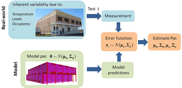
Figure 1. Graphical representation of the proposed hierarchical Bayesian framework.
In model updating applications, modeling bias (mean of modeling error) is commonly assumed to be zero. This assumption can be verified once the updating is completed by evaluating the error mean. If the error mean is negligible, then the assumption has been accurate. Therefore, the error function can be written as:
in which et is the error function for dataset t and consists of two parts: eigen-frequency error eλt and mode shape error eΦt, defined as:
Subscript m denotes the mode number, λm(θt)and Φm(θt) are model-predicted eigen-frequency (λm(θt)=(2πftm(θt))2, in which ftm(θt) is the natural frequency in Hz) and mode shape in dataset t, and ˜λtm and ˜Φtm are their identified counterparts. The natural frequencies and mode shapes extracted from the vibration measurement are referred to as identified modal parameters in this paper. Γis a Boolean matrix which maps corresponding degrees of freedom (DOFs) between Φm(θt) and ˜Φtm. atm is a scaling factor and defined as:
The assumption of μe = 0 considers negligible modeling bias, and in the case of significant modeling bias a non-zero μe should be considered. Due to the compensation effect between μθ and μe, these two terms cannot be estimated simultaneously. Therefore, μe is not updated through a Bayesian inference but is evaluated from the obtained results, as demonstrated in section Model updating with μe ≠ 0. The covariance matrix Σe is assumed to be a diagonal matrix which neglects the correlation between different error function components.
Note that a full matrix can also be estimated in this framework, but this would increase the computational burden of the updating process. Based on the authors' past experience, use of diagonal covariance matrix is reasonable in many applications. However, this is not true for all applications and errors in frequency and mode shape components of the same mode can be correlated. In the case of error function dependency, the estimated diagonal covariance matrix is an approximate solution of the full matrix.
The posterior probability density function (PDF) is proportional to the multiplication of the likelihood function and prior PDFs which are assumed to be independent (Gelman et al., 2013), as shown below:
Equation (7) is derived based on the fact that the identified modal parameters only depend on the structural stiffness θt and the error function, therefore, the condition on hyperparameters μθ and Σθ can be discarded from Equation (6). In addition, structural stiffness is only dependent on its hyperparameters, therefore, the condition on Σe can be dropped, and by assuming μθ, Σθ, and Σe are independent in their joint prior distribution, Equation (8) can be obtained. When multiple datasets are available and considered, the joint posterior PDF could be derived by assuming different datasets are independent:
where Θ = Θ=[θ1…θt…θNt],˜λ=[˜λ1…˜λt…˜λNt],˜Φ=[˜Φ1…˜Φt…˜ΦNt], and Nt denotes the number of datasets.
In this study, uniform prior PDF is assumed for μθ and “conjugate priors” (Gelman et al., 2013) are used for Σθ and Σe(σ2ei) to simplify the formulation as shown below.
In above equations, v1, v2, Σθ0, σ2e0 are the parameters of prior PDFs. The selection of these parameters can influence the final posterior distribution and should be made based on prior knowledge and engineering expertise. For the considered inverse-Wishart and Inverse- χ2 distributions, smaller values of v1 and v2 would “flatten/widen” the prior PDFs indicating larger prior uncertainties, and Σθ0 and σ2e0 would reflect the mode of distributions.
The joint posterior PDF is derived by substituting the likelihood function and conjugate prior PDFs into Equation (9) as shown below.
Here Np is the dimension of stiffness parameters θ, Ne is the dimension of error function et and is equal to (1 + Ns)Nm, and Nm and Ns denote number of available modes and number of components (sensors) of the identified mode shape, respectively.
The derived joint posterior PDF in Equation (13) is only known up to a normalizing constant, and it is often difficult to evaluate it analytically. Gibbs sampler, which belongs to the class of Markov Chain Monte Carlo (MCMC) methods, has been shown to be capable of sampling and evaluating Equation (13) efficiently. Gibbs sampler requires the derivation of posterior conditional PDFs which are listed below:
It can be seen that the posterior conditional PDFs for μθ, Σθ, and Σe are standard distributions due to the use of conjugate priors, therefore, samples can be easily generated for these parameters. However, the conditional PDF for θt is only known up to a scaling constant and therefore must be evaluated numerically. In this study, Metropolis-Hastings (MH) algorithm (Metropolis et al., 1953; Hastings, 1970) is employed to sample θt. The presented sampling algorithm is called MH within Gibbs sampler. Gibbs sampler samples the parameters recursively based on the conditional PDFs, and in each loop, one sample is generated containing the values of all updating parameters.
After the joint posterior PDF is evaluated using Gibbs sampler, the calibrated model can be used and assessed for prediction of structural dynamic behavior through propagating the uncertainties of inherent variability and modeling errors estimated in the hierarchical Bayesian framework. The parameter estimation uncertainties are not considered in this study, as this type of uncertainty becomes negligible when using larger amount of data. For prediction of natural frequencies and mode shapes, the definitions of error function in Equations (2, 3) are used:
where θt refers to the stiffness parameters of the calibrated model which follows the normal distribution N(ˆμθ,ˆΣθ) in which ˆμθ and ˆΣθ refer to the maximum a posteriori (MAP) values estimated through Gibbs sampler. The error function et (which consists of two parts eλtm and eΦtm) follows the normal distribution N(ˆμθ,ˆΣθ).
Accurate prediction of response time history is critical for assessment of structural performance by using metrics such as the maximum inter-story drift of buildings during an earthquake. Modal superposition method is employed to predict response time history. These predictions propagate uncertainties due to stiffness variability and modeling errors using the model-predicted modal parameters in Equations (22, 23). The equation of motion in modal coordinates (Chopra and Chopra, 2007) is:
where qm(t) is modal displacement of mode m, ωm is the circular natural frequency in rad/s and ωm=√λpretm, ζm is the damping ratio. Pm(t) is the generalized force function and Pm(t)=ΦTmP(t) in which P(t) is the input force vector. Mm is the generalized mass of mode m with Mm=ΦTmMΦm. The response time history in physical coordinates can be transformed from modal displacement as shown below:
In Equation (25), Nm denotes the total number of modes used in the model calibration process, which means that only contributions of Nm modes are included in the response predictions as the calibrated model is only sufficient for providing reliable predictions of these modes by propagating all uncertainties considered. Note that error function et is only evaluated at locations with measurement/sensors, which are usually sparse. To extend the error function to DOFs which are not measured, maximum component of ˆσe(ϕi,j) is assumed for unmeasured DOFs with μei = 0. This is a relatively conservative approach for the extension of error function. The velocity and acceleration prediction can be derived from Equation (25) by replacing qm with ˙qm or ¨qm. Note that the model-predicted displacement, velocity and acceleration responses are all relative to the ground.
The proposed hierarchical Bayesian approach is applied to a numerical model of a 10-story building for validation. The identified modal parameters of the building are simulated using a frame model as shown in Figure 2A. Foundation rocking is modeled by two rotational springs with stiffness kr=2× 10⁵kN-m/rad. The building is assumed to be 30 m (10 × 3 m) tall and 10 m wide with a total weight of 40 metric tons (each floor mass of 4 tons). No variability of the mass is considered in this study. The cross-section and Young's modulus of the columns and floor slabs are reported in Table 1. The larger values of Young's modulus for lower stories are representing larger effective Young's modulus of reinforced concrete at lower stories. To account for the inherent variability of the structural stiffness, Young's modulus of all members are assumed to follow normal distributions with means and standard deviations shown in Table 1. The stiffness of different structural members are independent except for the two columns on the same story which are assumed to have the same stiffness. The small rectangles with arrows in Figure 2A refer to the considered locations of accelerometers on the building and direction of measurements.
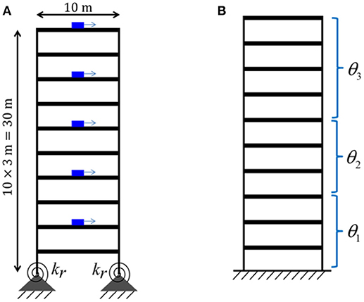
Figure 2. (A) 10-story frame model (exact); (B) 10-story shear building model (with modeling errors).
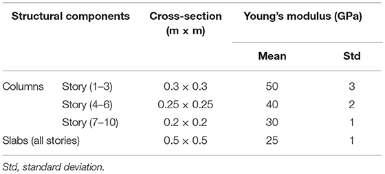
Table 1. Geometry and material property of the 10-story frame model.
Based on the assumed normal distribution of structural stiffness in the frame (exact) model, 100 sets of modal parameters (natural frequency and mode shape) are simulated, which represent the “measured” data. The modal parameters are polluted with white noise of 0.5% in coefficient of variation to account for the measurement noise and identification error. It is assumed that only the first three modes are identified and their histograms are shown in Figure 3. The mode shapes of the first three modes are shown in Figure 4, with mean stiffness assigned for all structural members in this graph. Note that 5 accelerometers are considered in the building, therefore, only mode shape components at these stories are available in the following model updating process.
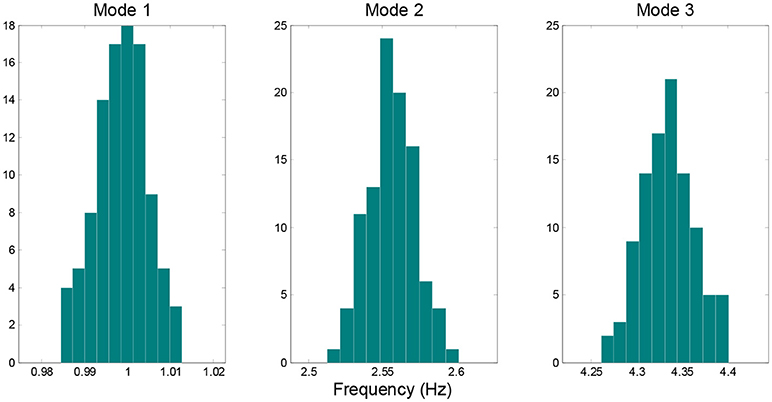
Figure 3. Histogram of simulated natural frequencies from the frame model.
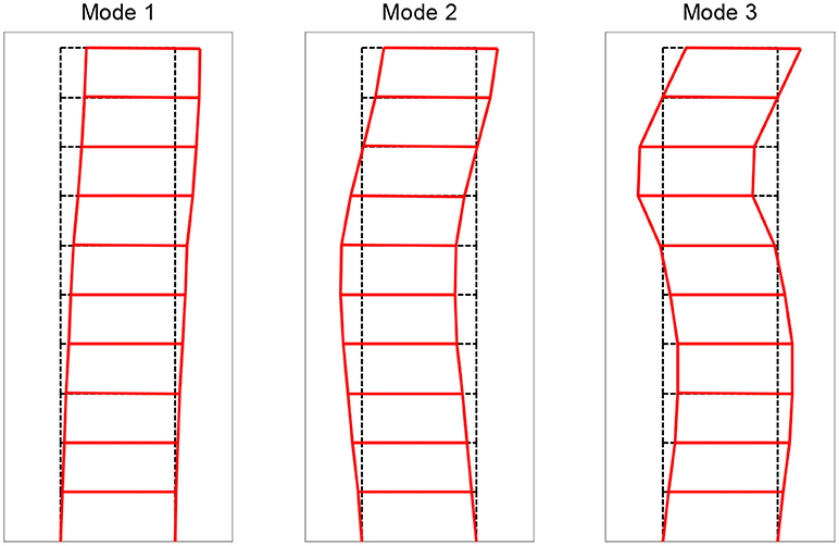
Figure 4. Simulated mode shapes of first three modes from the frame model.
To consider the effects of modeling errors, a 10-story shear building model (instead of a frame model) as shown in Figure 2B is used in the model updating process. In this model, the foundation rocking is ignored by using a fixed boundary condition, the floors motion is constrained as only horizontal direction, and the slabs are assumed to be rigid. The structural columns are grouped into three substructures (story 1–3, story 4–6, and story 7-10) as shown in Figure 2B, and the updating parameters θ1, θ2, and θ3 are the Young's modulus of columns in these substructures (the same Young's modulus is assumed for all columns in each group). It is assumed that the material distribution along the height of the building is known and can be divided into three groups. The substructuring strategy is utilized to limit the number of updating parameters. However, this strategy introduces additional modeling error due to the smearing effect of grouping strategy.
The proposed hierarchical Bayesian model updating approach is applied to estimate stiffness of the three substructures θ=[θ1,θ2,θ3]T, their hyperparameters μθ and Σθ, and covariance of error function Σe (mean of error function μe is assumed to be zero) using the simulated noisy modal parameters. After a tuning process, the parameters of prior PDFs in Equations (11, 12) are selected as:
MH within Gibbs sampler is employed to generate samples from the posterior conditional PDFs in Equations (16–19). In total, 20,000 samples are generated and first 5,000 samples are discarded as burn-in period to remove the transitional samples. Sample mean and standard deviation of μθ and Σθ are plotted in Figures 5, 6, which show that the samples have converged and the number of samples is adequate for estimating these statistics. The sample histograms for μθ, σθi, and σe(λ1−3) are shown in Figure 7. The black lines denote the kernel PDFs which are normalized to have the same height as the highest bins of the histograms and black dots denote the MAPs. The MAPs are estimated as the peaks of kernel PDFs which are preferred over selecting the sample with highest posterior probability to reduce the estimation uncertainty. Alternatively, the average values could be used but the MAPs are preferred as they represent the most probable values of parameters and are more appropriate for asymmetric distributions. It can be seen that samples of μθ seem to follow a normal distribution, samples of σθi roughly follow an Inverse-Wishart distribution, and samples of σe(λ1−3) approximately follow an Inverse- χ2 distribution with a tail on the right side. These are expected due to the choice of conjugate priors used in section Formulation of Hierarchical Bayesian Approach.
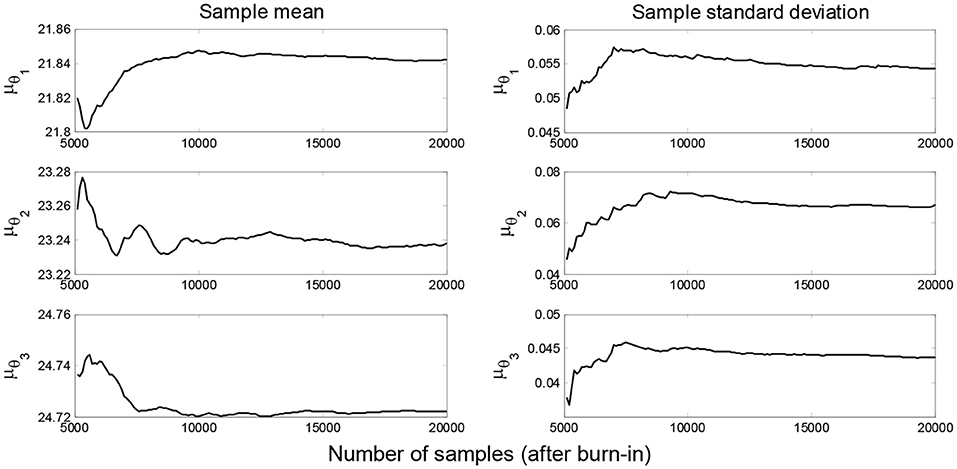
Figure 5. Sample mean and standard deviation of μθ.
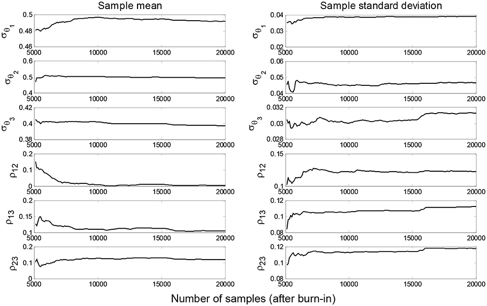
Figure 6. Sample mean and standard deviation of Σθ (ρ refers to correlation coefficient).
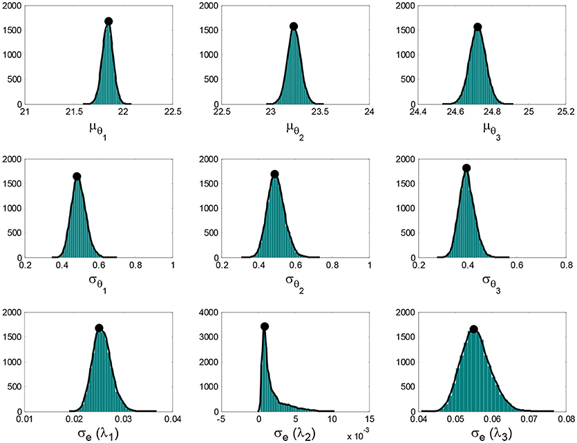
Figure 7. Histograms and kernel PDFs of μθ, σθi, and σe(λ1−3) (after burn-in).
The estimated MAPs of μθ, Σθ(σθi, ρij) and Σe(σei) are summarized in Table 2, together with their nominal values from the frame model. In Table 2, λi refers to eigen-frequency of mode i and ϕj, i refers to component j of mode shape i. It can be observed that and are underestimated compared to their nominal values due to the significant modeling errors introduced in the shear building model. Although the mean and standard deviation of stiffness are underestimated, the correlation coefficients are accurately estimated to be close to zero. Note that the overall stiffness variability in each of the three column groups is less than the individual stiffness uncertainty shown in Table 1 due to (1) the compensation effect of independent element stiffness, and more importantly (2) modeling errors in the shear building model, including the negligence of rocking behavior at the base and the rigid assumption of floors. The implemented grouping strategy introduces additional modeling errors. Grouping or sub-structuring is a common strategy to reduce the number of updating parameters and avoid unidentifiability/ill-conditioning.
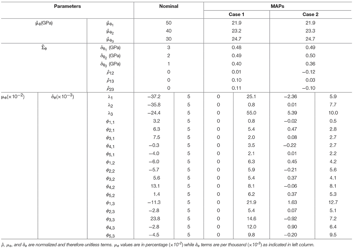
Table 2. MAPs of μθ, Σθ(σθi, ρij) and Σe(σei) for Case 1 (μe = 0) and Case 2 (μe ≠ 0), and evaluated μe from Case 1 results.
The updated structural parameters (Young's moduli) represent the effective stiffness of different substructures. In presence of large modeling errors, the updated values will compensate for non-updated model parameters and modeling errors, therefore, they may not correspond to the physical Young's modulus of the used material. In linear time-invariant applications, calibrated models can still provide good response prediction even outside the calibration range of response amplitude. However, the calibrated model should be cautiously used for prediction of local response quantities with little sensitivity to the used error metrics such as modal parameter errors. The available measurements can provide information about the accuracy or bias of the calibrated model on used error metrics (natural frequencies and mode shapes here). But they do not provide accurate estimation of the expected bias for localized quantities such as strains and stresses at locations with large modeling errors (e.g., base of the building in this application). Significant variability is observed for the covariance of error function, and and are estimated much larger than their nominal values (added white noise level of 0.5%) due to the modeling errors and the assumption of μe = 0 in Case 1. The nominal value of μe in Table 2 is computed based on the error function definition in Equations (2, 3) with Young's modulus the same as the mean values in Table 1.
The calibrated model is then used to predict the modal parameters using the formulation detailed in section Propagation of Uncertainties in Model-Predicted Response. A total of 1,000 natural frequency predictions are generated from the calibrated model and compared with their identified counterparts (simulated from the frame model) as shown in Figure 8. It can be observed that the range of identified values is fully covered by predictions. However, predictions have significantly larger variability than measured data. An evident difference is observed between the centers of two clouds (black dots vs. gray circles) which indicates error bias. Therefore, it is concluded that the assumption of μe = 0 is not an optimal choice in this case, and a non-zero μe is preferred. This observation prompts the second case of model updating referred to as Case 2 in the following section.
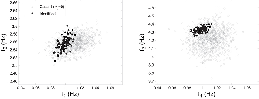
Figure 8. Comparison of natural frequency predictions with their identified counterparts using the calibrated model of Case 1 (μe = 0).
In this case of model updating, a non-zero mean is considered for the error function. Although μe cannot be updated simultaneously with μθ due to compensation effects, it can be evaluated from the observed bias in error function as shown below:
in which êtis the error function evaluated based on Equations (2, 3) using estimated in Case 1. A total of 100 different values of are estimated for 100 sets of modal parameters from the joint posterior distribution in Equation (13), and μe is computed as the mean of 100 evaluations of êt. The evaluated μe is reported in Table 2. It can be seen that the largest values in μe correspond to the natural frequencies of mode 1 and 3 which exhibit the largest bias in the predictions as shown in Figure 8. Note that the estimated bias does not provide physical interpretation of modeling errors, but it can potentially indicate the extent of such error.
The hierarchical Bayesian model updating is repeated with the evaluated value of μe from Equation (27). Note that in Case 2, μe is not updated through a Bayesian inference but is obtained using the updating results of Case 1. The model updating follows the same process with minor modifications in Equations (14, 21):
The estimated MAPs of μθ, Σθ(σθi, ρij), and Σe(σei) with μe ≠ 0 are reported in Table 2. It can be observed that and remain almost the same for the two cases which is expected because the hyperparameters estimation is based on the measured data and the underlying model. The inclusion of a constant μe only shifts the center of error function distribution and therefore, would not affect the hyperparameters. However, values of components are generally reduced, especially for and , making components much closer to their nominal values which are 0.005 due to the added white noise level of 0.5%. Similar comparison of natural frequency predictions with their identified counterparts using the calibrated model of Case 2 is shown in Figure 9. It can be seen that significantly improved predictions are achieved in this case compared to Figure 8. No observable bias exists between the two clouds (black dots vs. gray circles), and similar variability is observed. This demonstrates the importance of accounting for modeling bias in the proposed hierarchical Bayesian framework to achieve more accurate predictions.
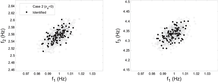
Figure 9. Comparison of natural frequency predictions with their identified counterparts using the calibrated model of Case 2 (μe ≠ 0).
The calibrated models from Case 1 and Case 2 are used to predict response time history to an earthquake ground motion using the modal superposition method described in section Propagation of Uncertainties in Model-Predicted Response. The input is the recorded ground motion at Antrodoco station during the 2009 L'Aquila Italy earthquake as shown in Figure 10. The response predictions only include the contribution of the first three modes as the shear building model is only calibrated using these modes. The building is assumed to have modal damping ratios of 2% for all modes. To account for the estimation uncertainty of damping ratios, the identified damping ratios of the first three modes are assumed to be 2% with a coefficient of variation of 30%. Therefore, response time history predictions include the uncertainties of the estimated stiffness inherent variability (), uncertainty of error function () and the uncertainty of damping ratios. To verify the accuracy of response predictions, the model predictions are compared with the response of the exact (frame) model. The damping of the frame mode is assumed to be exact (2% damping ratios for all modes) and the contributions of all modes are included in the simulation. However, the exact model simulations consider the variability of stiffness parameters using their exact probability distributions. It is worth noting that under large amplitude seismic excitations, buildings experience non-linear hysteretic behavior (Astorga et al., 2018). Therefore, in the case of dealing with large amplitude excitations, a non-linear model of the structural system is recommended to be used. The proposed hierarchical Bayesian method can then be applied for non-linear model calibration where hysteretic material properties can be considered as updating parameters. However, in this study the considered ground motion is deliberately selected to have a small peak ground acceleration of around 0.02 g so the assumption of linear elastic regime with low damping is realistic. Furthermore, certain building codes allow the use of linear FE models for simplified and approximate analysis of buildings under seismic loads such as the equivalent linear procedure and response spectrum procedure. These two linear methods are routinely used in practice to predict structural responses during seismic events.
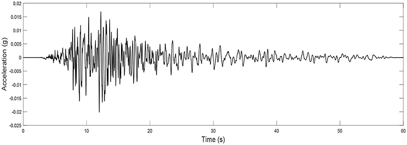
Figure 10. Acceleration record of the 2009 L'Aquila Italy earthquake.
A total of 200 independent predictions (using calibrated model) and simulations (using exact model) are performed and a 95% confidence interval is generated by: (1) sorting the 200 values at each time instant in an increasing order; (2) selecting the 6th and 195th values as the lower and upper bounds of the confidence interval. Note that only 5 sensors (story 2, 4, 6, 8, and 10) are considered in the model updating process, therefore, the estimated error function only includes information for these stories. The error function is extended for unmeasured DOFs using the strategy detailed in section Propagation of Uncertainties in Model-Predicted Response to predict response of the unmeasured DOFs. The comparisons of displacement and acceleration time history predictions at the roof with their simulated counterparts are shown in Figures 11, 12. A good agreement is observed between model predictions and simulations for both cases, while the predictions in Case 2 are more accurate (smaller bias and uncertainty). Note that in general, acceleration predictions have larger uncertainty compared to displacements since a larger number of modes contribute to acceleration response and higher modes often have larger modeling errors. In this study, accelerations are predicted using only the first three modes while the simulations of true response include contributions of all modes. Figures 13, 14 show the model-predicted responses at the 7th floor which does not have a sensor. Again, a good agreement can be seen for displacement and acceleration time history predictions and simulated response. Similarly, Case 2 predictions provide tighter fit with simulated response. In general, the predictions in DOFs without sensors are more conservative (larger variance) due to the conservative assumption made in the extension of error functions detailed in section Propagation of Uncertainties in Model-Predicted Response. The statistics of maximum roof displacement, maximum roof acceleration and maximum inter-story drift of the 10th story for measurement and predictions of Case 1 and Case 2 are summarized in Table 3. It can be seen that, although Case 1 provides relative satisfactory results, Case 2 delivers significantly more accurate mean values and standard deviations.
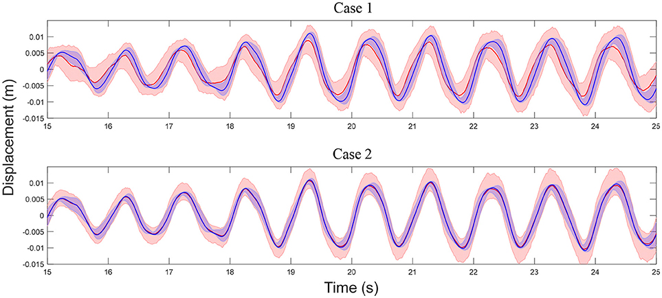
Figure 11. Comparison of displacement time history predictions at story 10 with measurements (simulations) for Case 1 and Case 2. Light red shaded area: 95% confidence interval of predictions, blue shaded area: 95% confidence interval of simulations, red line: median of predictions, blue line: median of simulations.
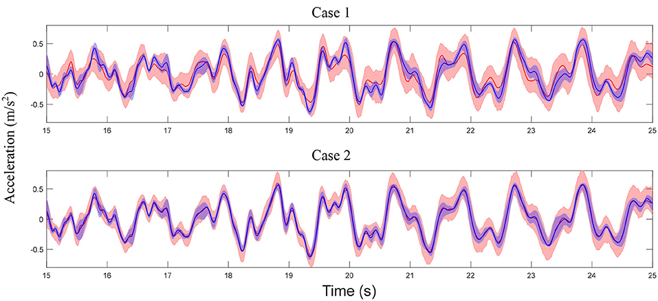
Figure 12. Comparison of acceleration time history predictions at story 10 with measurements for Case 1 and Case 2 (refer to Figure 11 for legends).
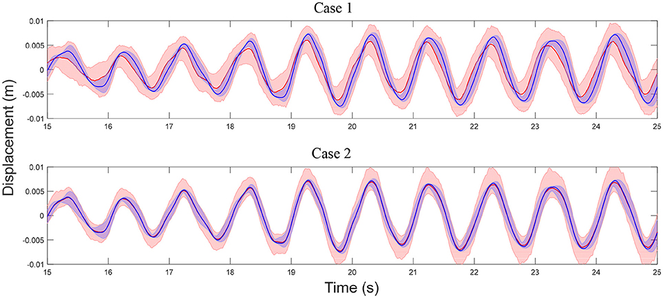
Figure 13. Comparison of displacement time history predictions at story 7 (no sensor/measurement) with measurements for Case 1 and Case 2 (refer to Figure 11 for legends).
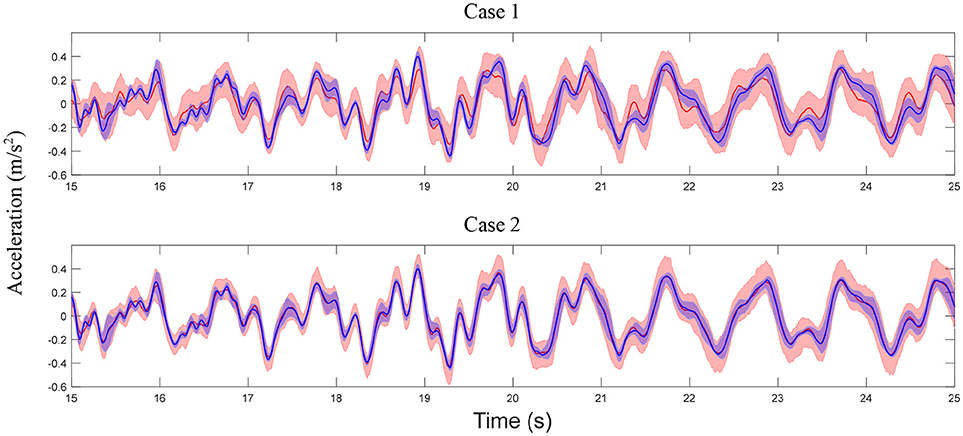
Figure 14. Comparison of acceleration time history predictions at story 7 (no sensor/measurement) with measurements for Case 1 and Case 2 (refer to Figure 11 for legends).
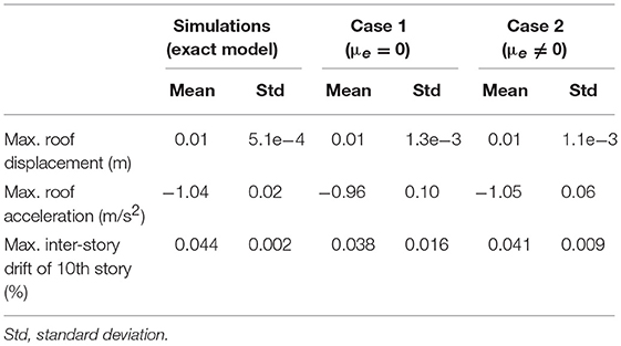
Table 3. Statistics of maximum roof displacement, maximum roof acceleration, and maximum inter-story drift of 10th story for measurement and predictions.
In this paper a hierarchical Bayesian model updating approach is implemented for modeling error estimation and response prediction of a 10-story building model using modal parameters. The identified modal parameters are simulated from a frame model which represents the true structure. A shear building model with significant modeling errors is created for model updating and the stiffness of three defined substructures are selected as updating parameters. The hierarchical Bayesian approach is employed to estimate the stiffness mean and covariance, as well as the modeling errors of the shear building model. Metropolis-Hastings within Gibbs sampler is implemented to evaluate numerically the joint posterior distribution of updating parameters. The mean of error function μe is first assumed to be zero in Case 1. Evident bias is observed in natural frequency predictions which prompts a second case of model updating (Case 2) with μe evaluated from the observed bias. The natural frequency predictions for Case 2 show no bias and similar variability to the identified values. Displacement and acceleration time history predictions are obtained for both cases and for all measured and unmeasured DOFs. Good agreements are observed between predictions and measurements for both cases and for all DOFs. The predictions are improved significantly for Case 2 when considering non-zero modeling bias. These observations validate the proposed hierarchical Bayesian approach for model calibration, modeling error estimation, and response prediction by considering and propagating the uncertainties of structural stiffness and modeling errors, and demonstrate the effects of accounting for modeling bias in response predictions. In the application of proposed hierarchical Bayesian method, model updating is recommended to initially be applied with the assumption of zero mean error (similar to Case 1). If evident prediction error bias is observed from the calibrated model, then a second case can be applied to remove the bias and improve the predictions. The main novelties of the proposed approach include the following.
(I) The “inherent variability” of updating structural parameters (stiffness) due to changing ambient and environmental conditions is quantified and estimated by the hyperparameters μθ and Σθ. As expected, the parameter estimation uncertainties would decrease with additional data but the estimated inherent variabilities would converge to a constant value similar to the estimation variability obtained from a frequentist approach. This is not the case for traditional Bayesian approaches.
(II) Modeling errors are characterized by a joint normal distribution with mean μe and covariance Σe and are propagated in model predictions. In the case of considering zero modeling bias μe, the covariance term will be overestimated to compensate for the bias, resulting in larger confidence intervals on model predictions.
(III) In presence of significant modeling errors, the effective structural parameters can be under/over-estimated, but the calibrated model can still provide accurate confidence intervals on response predictions due to the inclusion of modeling errors.
MS is the lead author where he completed most of the study and composed the paper. IB provided technical feedback for implementing the framework and sampling. BM serves as MS supervisor and provided guidance through the study as well as polishing the text. CP also provided feedback on technical details of the updating framework.
The authors declare that the research was conducted in the absence of any commercial or financial relationships that could be construed as a potential conflict of interest.
Partial support of this study by the National Science Foundation Grant 1254338 is gratefully acknowledged. The opinions, findings, and conclusions expressed in this paper are those of the authors and do not necessarily represent the views of the sponsors and organizations involved in this project.
Alampalli, S. (2000). Effects of testing, analysis, damage, and environment on modal parameters. Mech. Syst. Signal Process. 14, 63–74. doi: 10.1006/mssp.1999.1271
Astorga, A., Guéguen, P., and Kashima, T. (2018). Nonlinear elasticity observed in buildings during a long sequence of earthquakes. Bull. Seismol. Soc. Am. 108, 1185–1198. doi: 10.1785/0120170289
Bakir, P. G., Reynders, E., and De Roeck, G. (2008). An improved finite element model updating method by the global optimization technique ‘Coupled Local Minimizers’. Comput. Struct. 86, 1339–1352.
Beck, J. L., and Au, S.-K. (2002). Bayesian updating of structural models and reliability using Markov chain Monte Carlo simulation. J. Eng. Mech. 128, 380–391. doi: 10.1061/(ASCE)0733-9399(2002)128:4(380)
Beck, J. L., Au, S. K., and Vanik, M. W. (2001). Monitoring structural health using a probabilistic measure. Comput. Aided Civil Infrastruct. Eng. 16, 1–11. doi: 10.1111/0885-9507.00209
Beck, J. L., and Katafygiotis, L. S. (1998). Updating models and their uncertainties. I: bayesian statistical framework. J. Eng. Mech. 124, 455–461. doi: 10.1061/(ASCE)0733-9399(1998)124:4(455)
Behmanesh, I., and Moaveni, B. (2015). Probabilistic identification of simulated damage on the Dowling Hall footbridge through Bayesian finite element model updating. Struct. Control Health Monit. 22, 463–483. doi: 10.1002/stc.1684
Behmanesh, I., and Moaveni, B. (2016). Accounting for environmental variability, modeling errors, and parameter estimation uncertainties in structural identification. J. Sound Vib. 374, 92–110. doi: 10.1016/j.jsv.2016.03.022
Behmanesh, I., Moaveni, B., Lombaert, G., and Papadimitriou, C. (2015). Hierarchical Bayesian model updating for structural identification. Mech. Syst. Signal Process. 64, 360–376. doi: 10.1016/j.ymssp.2015.03.026
Brownjohn, J. M., and Xia, P.-Q. (2000). Dynamic assessment of curved cable-stayed bridge by model updating. J. Struct. Eng. 126, 252–260. doi: 10.1061/(ASCE)0733-9445(2000)126:2(252)
Brownjohn, J. M. W., Moyo, P., Omenzetter, P., and Yong, L. (2003). Assessment of highway bridge upgrading by dynamic testing and finite-element model updating. J. Bridge Eng. 8, 162–172. doi: 10.1061/(ASCE)1084-0702(2003)8:3(162)
Capecchi, D., and Vestroni, F. (1993). Identification of finite element models in structural dynamics. Eng. Struct. 15, 21–30. doi: 10.1016/0141-0296(93)90013-T
Ching, J., and Beck, J. L. (2004). New Bayesian model updating algorithm applied to a structural health monitoring benchmark. Struct. Health Monitoring 3, 313–332. doi: 10.1177/1475921704047499
Ching, J., and Chen, Y.-C. (2007). Transitional Markov chain Monte Carlo method for Bayesian model updating, model class selection, and model averaging. J. Eng. Mech. 133, 816–832. doi: 10.1061/(ASCE)0733-9399(2007)133:7(816)
Chopra, A. K., and Chopra, A. K. (2007). Dynamics of Structures: Theory and Applications to Earthquake Engineering. Saddle River, NJ: Pearson/Prentice Hall Upper.
Clinton, J. F., Bradford, S. C., Heaton, T. H., and Javier, F. (2006). The observed wander of the natural frequencies in a structure. Bull. Seismol. Soc. Am. 96, 237–257. doi: 10.1785/0120050052
Fang, S.-E., Perera, R., and De Roeck, G. (2008). Damage identification of a reinforced concrete frame by finite element model updating using damage parameterization. J. Sound Vib. 313, 544–559. doi: 10.1016/j.jsv.2007.11.057
Friswell, M., and Mottershead, J. E. (2013). Finite Element Model Updating in Structural Dynamics. Berlin: Springer Science & Business Media.
Friswell, M. I., Mottershead, J. E., and Ahmadian, H. (2001). Finite–element model updating using experimental test data: parametrization and regularization. Philos. Trans. R. Soc. London A Math. Phys. Eng. Sci. 359, 169–186. doi: 10.1098/rsta.2000.0719
Gelman, A., Carlin, J. B., Stern, H. S., Dunson, D. B., Vehtari, A., and Rubin, D. B. (2013). Bayesian Data Analysis. New York, NY: Chapman and Hall/CRC.
Goulet, J.-A., Michel, C., and Smith, I. F. (2013). Hybrid probabilities and error-domain structural identification using ambient vibration monitoring. Mech. Syst. Signal Process. 37, 199–212. doi: 10.1016/j.ymssp.2012.05.017
Goulet, J.-A., and Smith, I. F. (2013). Structural identification with systematic errors and unknown uncertainty dependencies. Comput. Struct. 128, 251–258. doi: 10.1016/j.compstruc.2013.07.009
Hastings, W. K. (1970). Monte Carlo sampling methods using Markov chains and their applications. 57, 97–109. doi: 10.1093/biomet/57.1.97
Jafarkhani, R., and Masri, S. F. (2011). Finite element model updating using evolutionary strategy for damage detection. Comp. Aided Civil Infrastruct. Eng. 26, 207–224. doi: 10.1111/j.1467-8667.2010.00687.x
Jaishi, B., Kim, H.-J., Kim, M. K., Ren, W. W., and Lee, S. H. (2007). Finite element model updating of concrete-filled steel tubular arch bridge under operational condition using modal flexibility. Mech. Syst. Signal Process. 21, 2406–2426. doi: 10.1016/j.ymssp.2007.01.003
Jaishi, B., and Ren, W.-X. (2006). Damage detection by finite element model updating using modal flexibility residual. J. Sound Vib. 290, 369–387. doi: 10.1016/j.jsv.2005.04.006
Katafygiotis, L. S., and Beck, J. L. (1998). Updating models and their uncertainties. II: model identifiability. J. Eng. Mech. 124, 463–467. doi: 10.1061/(ASCE)0733-9399(1998)124:4(463)
Levin, R., and Lieven, N. (1998). Dynamic finite element model updating using simulated annealing and genetic algorithms. Mech. Syst. Signal Process. 12, 91–120. doi: 10.1006/mssp.1996.0136
Metropolis, N., Rosenbluth, A. W., Rosenbluth, M. N., Teller, A. H., and Teller, E. (1953). Equation of state calculations by fast computing machines. J. Chem. Phys. 21, 1087–1092. doi: 10.1063/1.1699114
Moaveni, B., Stavridis, A., Lombaert, G., Conte, J. P., and Shing, P. B. (2012). Finite-element model updating for assessment of progressive damage in a 3-story infilled RC frame. J. Struct. Eng. 139, 1665–1674. doi: 10.1061/(ASCE)ST.1943-541X.0000586
Moser, P., and Moaveni, B. (2011). Environmental effects on the identified natural frequencies of the Dowling Hall Footbridge. Mech. Syst. Signal Process. 25, 2336–2357. doi: 10.1016/j.ymssp.2011.03.005
Mottershead, J. E., and Friswell, M. (1993). Model updating in structural dynamics: a survey. J. Sound Vib. 167, 347–375. doi: 10.1006/jsvi.1993.1340
Muto, M., and Beck, J. L. (2008). Bayesian updating and model class selection for hysteretic structural models using stochastic simulation. J. Vib. Control 14, 7–34. doi: 10.1177/1077546307079400
Ntotsios, E., Papadimitriou, C., Panetsos, P., Karaiskos, G., Perros, K., and Perdikaris, P. C. (2009). Bridge health monitoring system based on vibration measurements. Bull. Earthq. Eng. 7:469. doi: 10.1007/s10518-008-9067-4
Pai, S. G., Nussbaumer, A., and Smith, I. F. (2018). Comparing structural identification methodologies for fatigue life prediction of a highway bridge. Front. Built Environ. 3:73. doi: 10.3389/fbuil.2017.00073
Pasquier, R., and Smith, I. F. (2015). Robust system identification and model predictions in the presence of systematic uncertainty. Adv. Eng. Informatics 29, 1096–1109. doi: 10.1016/j.aei.2015.07.007
Perera, R., and Ruiz, A. (2008). A multistage FE updating procedure for damage identification in large-scale structures based on multiobjective evolutionary optimization. Mech. Syst. Signal Process. 22, 970–991. doi: 10.1016/j.ymssp.2007.10.004
Reuland, Y., Lestuzzi, P., and Smith, I. F. (2017). Data-interpretation methodologies for non-linear earthquake response predictions of damaged structures. Front. Built Environ. 3:43. doi: 10.3389/fbuil.2017.00043
Reynders, E., Roeck, G. D., Gundes Bakir, P., and Sauvage, C. (2007). Damage identification on the Tilff Bridge by vibration monitoring using optical fiber strain sensors. J. Eng. Mech. 133, 185–193. doi: 10.1061/(ASCE)0733-9399(2007)133:2(185)
Sohn, H., and Law, K. H. (1997). A Bayesian probabilistic approach for structure damage detection. Earthq. Eng. Struct. Dynam. 26, 1259–1281. doi: 10.1002/(SICI)1096-9845(199712)26:12<1259::AID-EQE709>3.0.CO;2-3
Song, M., Renson, L., Noël, J. P., Moaveni, B., and Kerschen, G. (2018). Bayesian model updating of nonlinear systems using nonlinear normal modes. Struct. Control Health Monit. 25:e2258. doi: 10.1002/stc.2258
Song, M., Yousefianmoghadam, S., Mohammadi, M.-E., Moaveni, B., Stavridis, A., and Wood, R. L. (2017). An application of finite element model updating for damage assessment of a two-story reinforced concrete building and comparison with lidar. Struct. Health Monit. 17, 1129–1150. doi: 10.1177/1475921717737970
Teughels, A., and De Roeck, G. (2004). Structural damage identification of the highway bridge Z24 by FE model updating. J. Sound Vib. 278, 589–610. doi: 10.1016/j.jsv.2003.10.041
Teughels, A., De Roeck, G., and Suykens, J. A. (2003). Global optimization by coupled local minimizers and its application to FE model updating. Comput. Struct. 81, 2337–2351. doi: 10.1016/S0045-7949(03)00313-4
Teughels, A., Maeck, J., and De Roeck, G. (2002). Damage assessment by FE model updating using damage functions. Comput. Struct. 80, 1869–1879. doi: 10.1016/S0045-7949(02)00217-1
Yuen, K. V., Beck, J. L., and Au, S. K. (2004). Structural damage detection and assessment by adaptive Markov chain Monte Carlo simulation. Struct. Control Health Monit. 11, 327–347. doi: 10.1002/stc.47
Keywords: hierarchical Bayesian model updating, modeling error estimation, uncertainty quantification and propagation, probabilistic response prediction, Metropolis-Hastings within Gibbs sampler
Citation: Song M, Behmanesh I, Moaveni B and Papadimitriou C (2019) Modeling Error Estimation and Response Prediction of a 10-Story Building Model Through a Hierarchical Bayesian Model Updating Framework. Front. Built Environ. 5:7. doi: 10.3389/fbuil.2019.00007
Received: 17 October 2018; Accepted: 11 January 2019;
Published: 31 January 2019.
Edited by:
Ian F. C. Smith, École Polytechnique Fédérale de Lausanne, SwitzerlandReviewed by:
Feng-Liang Zhang, Tongji University, ChinaCopyright © 2019 Song, Behmanesh, Moaveni and Papadimitriou. This is an open-access article distributed under the terms of the Creative Commons Attribution License (CC BY). The use, distribution or reproduction in other forums is permitted, provided the original author(s) and the copyright owner(s) are credited and that the original publication in this journal is cited, in accordance with accepted academic practice. No use, distribution or reproduction is permitted which does not comply with these terms.
*Correspondence: Babak Moaveni, babak.moaveni@tufts.edu
Disclaimer: All claims expressed in this article are solely those of the authors and do not necessarily represent those of their affiliated organizations, or those of the publisher, the editors and the reviewers. Any product that may be evaluated in this article or claim that may be made by its manufacturer is not guaranteed or endorsed by the publisher.
Research integrity at Frontiers
Learn more about the work of our research integrity team to safeguard the quality of each article we publish.