 Koki Makita
 Izuru Takewaki
94% of researchers rate our articles as excellent or good
Learn more about the work of our research integrity team to safeguard the quality of each article we publish.
Find out more
ORIGINAL RESEARCH article
Front. Built Environ., 22 January 2019
Sec. Earthquake Engineering
Volume 5 - 2019 | https://doi.org/10.3389/fbuil.2019.00002
This article is part of the Research TopicInnovative Methodologies for Resilient Buildings and CitiesView all 9 articles
It is known that, while the stochastic Green's function method is suitable for generating ground motions with short periods, the three-dimensional finite difference method (FDM) is appropriate for ground motions with rather long periods. In the previous research, the stochastic Green's function method was used for finding the critical earthquake ground motion for variable fault rupture slip (slip distribution and rupture front). However, it cannot be used for ground with irregularities and for wave component with rather long periods. In responding to this request, the FDM is used in this paper for finding the critical ground motion for structures with rather long natural period. Since the FDM is time-consuming, it seems unfavorable to use it in a simple sensitivity algorithm where an independent response sensitivity is calculated for many design parameters. To overcome this difficulty, the bi-cubic spline interpolation of uncertain parameter distributions (seismic moment distribution in this paper) and the response surface method for predicting the response surface from some sampling points are used effectively in this paper. The uncertainty parameter is the fault rupture slip distribution described in terms of seismic moments. It is found that the critical ground motion for structures with rather long natural period can be found effectively by the proposed method.
There was common understanding that earthquake ground motions can be classified into a few types (Abrahamson et al., 1998). However, many earthquake ground motions of peculiar characteristics have been observed recently in the world (for example, Mexico, 1985; Northridge, 1994; Kobe, 1995; Chi-chi, 1999; Tohoku, 2011). After such earthquakes occur, we feel that unpredictable ground motions can occur and powerful theoretical approaches are inevitable to respond to those ground motions. One of the approaches may be the critical excitation method (see Drenick, 1970; Takewaki, 2007) which enables the search of the worst earthquake ground motion among possible ones. To tackle the worst ground motion under the consideration of fault rupture models, tools for producing ground motions in terms of fault rupture models may be necessary (Makita et al., 2018b).
It is well recognized that, while the empirical Green's function method (Irikura, 1986; Yokoi and Irikura, 1991) or the stochastic Green's function method (Wennerberg, 1990; Hisada, 2008) is suitable for generating ground motions with short periods, the three-dimensional finite difference method (FDM) is appropriate for ground motions with rather long periods (Bouchon, 1981; Hisada and Bielak, 2003; Yoshimura et al., 2003; Nickman et al., 2013). To enhance the usability of the FDM, an open software (GMS: Ground Motion Simulator) is available (Aoi and Fujiwara, 1999; Aoi et al., 2008; Maeda et al., 2012, 2016; Tanaka et al., 2014). The combination of these two-type motions with the use of a matching filter is acknowledged as the most powerful and reliable method for generating earthquake ground motions under the consideration of fault ruptures and surface waves. Since the parameters used in these methods for ground motion generation contain various uncertainties, i.e., aleatory uncertainty and epistemic uncertainty (Taniguchi and Takewaki, 2015; Okada et al., 2016), the treatment of such uncertainties are essential for the reliable estimation of ground motions (Abrahamson et al., 1998; Lawrence Livermore National Laboratory, 2002; Morikawa et al., 2008; Cotton et al., 2013).
In the previous research (Makita et al., 2018a), the effect of the fault rupture was taken into account simply by introducing the phase difference method. The robustness of a new building structural system consisting of base-isolation and building connection (Murase et al., 2013) was investigated for uncertain ground models. However, the fault rupture mechanisms cannot be considered in detail. In another previous research (Makita et al., 2018b), the stochastic Green's function method was used for finding the critical earthquake ground motion for variable fault rupture slip (slip distribution and rupture front). However, it cannot be used for ground with irregularities and for wave component with rather long periods.
Since the FDM is time-consuming, it seems unfavorable to use it in a simple sensitivity algorithm where an independent response sensitivity is calculated for each design parameter. To overcome this difficulty, the bi-cubic spline interpolation of uncertain parameter distributions (seismic moment distribution in this paper) through the control points and the response surface method for predicting the response surface from some sampling points are used effectively in this paper. The uncertain parameter is the fault rupture slip distribution described in terms of seismic moments at the control points. It is found that the critical ground motion for building structures with rather long natural period can be found effectively by the proposed method.
To investigate the effect of uncertainty level in the fault rupture on the robustness of building structures using the robustness function (Ben-Haim, 2006), several uncertainty levels are set and the critical fault rupture model is sought. Then the maximum story ductility is obtained for each uncertainty level.
In this paper, the uncertain parameter is the fault rupture slip distribution described in terms of seismic moments M0. First of all, the nominal distribution of fault rupture slip is given. The rupture front is assumed to develop concentrically as shown in Figure 1A. To reduce the degree of freedom in the setting of variable fault rupture slip distribution, some control points are selected in the fault. Sampling points in the uncertain parameter range are planned by the experimental design method at all control points. Then the uncertain parameters at all points are interpolated from the values at the control points by introducing bi-cubic spline interpolation of uncertain parameter distributions (seismic moment distribution in this paper). In the next, ground motions are generated by using the FDM. The response of a structure under the generated ground motion is computed. Then the response surface is obtained by the least-squares method. The maximum value of the response surface is determined by using the Sequential Quadratic Programming (SQP) method. Finally, the critical fault model is found and the corresponding ground motion is generated. The earthquake response analysis is conducted under the critical ground motion. The flowchart for finding the critical earthquake ground motion is shown in Figure 1B. To investigate the robustness of a building structure with rather long natural period with respect to the variability of the fault rupture distribution, the robustness function due to Ben-Haim (2006) is introduced. The relation of the maximum response of the structure with the uncertainty level of variable fault rupture slip distribution provides the quantitative evaluation of the robustness of the structure against the uncertain environment.
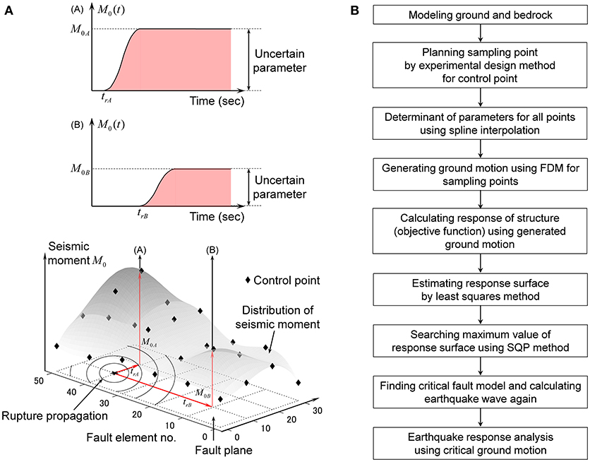
Figure 1. Outline of proposed method. (A) Scheme of setting variable seismic moment distribution in fault. (B) Flowchart for finding critical earthquake ground motion.
As mentioned above, in the generation of ground motions, FDM is used for producing ground motions with rather long periods (usually longer than about 1–2s). For ground motion components with shorter periods, the stochastic Green's function method is often used. Then both ground motion components are combined with the matching filter. Since a building structure with a rather long fundamental natural period is treated here, FDM is employed for generating ground motions.
The three-dimensional finite difference method (FDM) is often used as a useful numerical method for generating earthquake ground motions on the ground with irregularities. It can also take the fault rupture mechanism into consideration. In the research group of ground motion generation, an open source (GMS: Ground Motion Simulator: http://www.gms.bosai.go.jp/GMS/) can be used (Aoi and Fujiwara, 1999; Aoi et al., 2008; Maeda et al., 2012, 2016; Tanaka et al., 2014). In this paper, such open source software is used. The reliability and accuracy of this software will be investigated through the comparison with actual earthquake events and the benchmark tests (see Appendix).
The response surface method (RSM) is often used as an efficient and reliable method for prediction of responses of structures with many parameters (Khuri and Cornell, 1996). The procedure of the RSM can be summarized as follows: (i) Select the control points, (ii) Plan sampling points by the experimental design method for the control points, (iii) Interpolate the uncertain parameters at all points from the values at the control points, (iv) Generate ground motion using the FDM, (v) Calculate the response of a structure under the generated ground motion (vi) Estimate the response surface by the least-squares method, (vii) Search the maximum value of the response surface using the SQP method.
While the earthquake ground motions have to be generated repeatedly in the design procedure based on the conventional critical excitation method after the change of design conditions (the change of uncertainty level in the fault as treated in this paper or the change of superstructures etc.), those do not need to be generated in the design procedure based on the proposed critical excitation method using the RSM. This is because the earthquake ground motions for given sampling points have been generated and those can be used repeatedly.
Let xi denote the seismic moment at the control point i. The response surface in terms of quadratic functions can be expressed as
where the first term is a linear term, the second term is a quadratic term, the third term is a cross term, the fourth term c0 is a constant, and the fifth term ε is an error term. ci, , cij are their coefficients.
Although the second-order approximation is said to be inferior to the third-order approximation, it has some merits, (i) the required number of sampling points for a given accuracy is small, (ii) the solution is stable, (iii) the computational load for the increasing number of input factors is within a reasonable range. The coefficients ci, , cij, c0 are determined by using the well-known least-squares method.
In the next, let us explain the sampling method for the second-order approximation. The representative methods are (i) Latin Hypercube Sampling (LHS), (ii) Central Composite Design (CCD), (iii) Box-Behnken Design (BBD) (see Box and Behnken, 1960). Among these sampling methods, CCD, and BBD are designed for the evaluation of the second-order approximation. Figure 2A shows the CCD sampling method for three parameters. Each axis indicates the variation of the corresponding uncertain parameter. In the CCD method, the necessary number of sampling points for n uncertain parameters is (n + 2)(n + 1)/2 (Ohbuchi et al., 2011). In this paper, CCD method is employed.
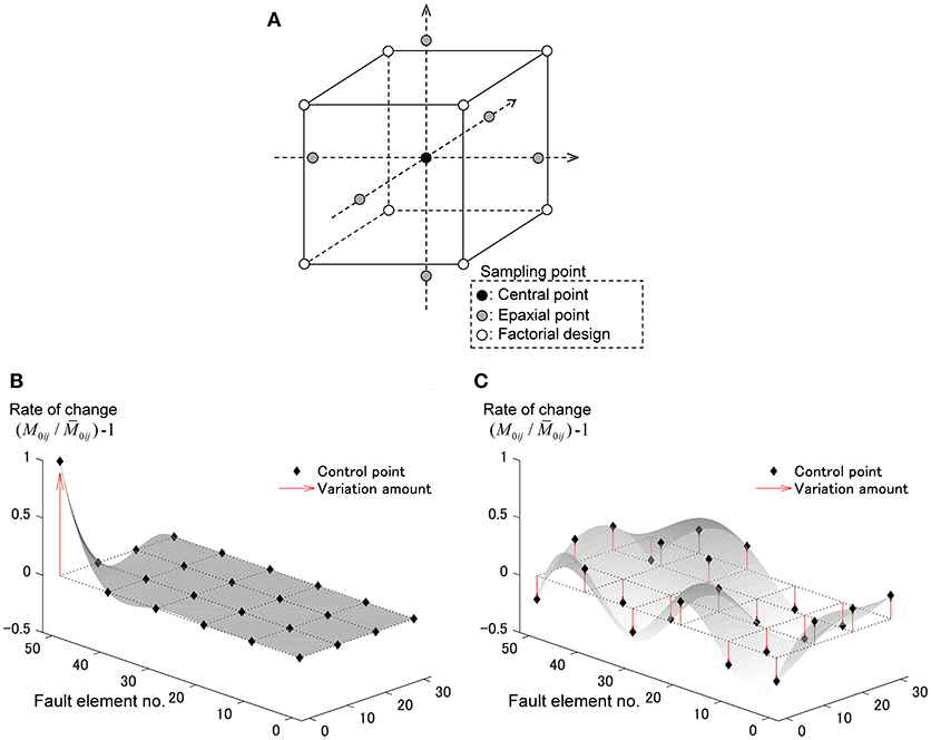
Figure 2. Expression of variability in seismic moment allocated to fault element for response surface method. (A) Schematic diagram of three-dimensional Central Composite Design (CCD). (B) Example of epaxial point. (C) Example of factorial design.
In CCD, three types of sampling points exist, (i) Central point, (ii) Epaxial point, (iii) Factorial design. Let M0ij and denote the seismic moment and its nominal value. The central point indicates a nominal value. The Epaxial point, , is on an axis and it varies the range (−1, 1) as shown in Figure 2B. Figure 2B shows an example such that the value only at the point (1, 5) varies. Since the Factorial design is intended to interact with each other, it makes each parameter vary as shown in Figure 2C. The objective of the Factorial design is to investigate the interaction between parameters.
If the number of divisions in the fault plane is small, the FDM cannot simulate the smooth fault rupture and keep the computational accuracy in a wide frequency range. When we consider many uncertain parameters in a fault plane, the robustness evaluation needs formidable amount of computational load. Therefore, some techniques are needed to reduce the computational load.
The seismic moment distribution at all points is obtained by using the bi-cubic spline interpolation for the seismic moments at the control points. Consider the fault element in the region [pi, pi+1] × [qj, qj+1]. The seismic moment in this region can be expressed by
where is the coefficient. The method of setting of the bi-cubic spline functions is explained in Figures 3A–F. The respective procedures (a)-(f) can be summarized as follows.
(a) Set the rectangular fault model (nominal model). All the fault elements in this nominal model have a constant seismic moment. Select some control points.
(b) Vary the seismic moments at these control points within a specified range.
(c) Interpolate the seismic moments at all points (element fault points) from the values at the control points by using the bi-cubic spline functions.
(d) Detect the value M0ij all points from the bi-cubic spline functions. If M0ij < 0 is detected, 0 is given.
(e) Set the asperity from the obtained seismic moment distribution. Select sequentially as an asperity from the fault element with the largest seismic moment.
(f) When the total seismic moment attains 70% of the preassigned seismic moment of the overall fault or the total area of the asperities becomes over 22% of the fault area, terminate the selection of the asperities. Modify the rise time of the selected asperities.
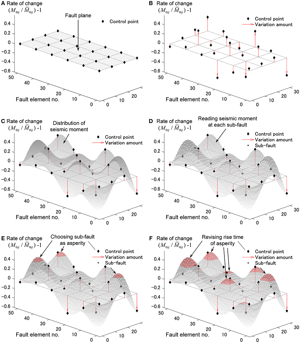
Figure 3. Process of constructing critical fault model (variation of seismic moment in each fault element). (A) Setting of nominal model. (B) Variation of seismic moment at control point. (C) Interpolation of seismic moments at all points from values at control points. (D) Determination of seismic moments at all points by using bi-cubic spline function. (E) Set the asperity from the obtained seismic moment distribution. (F) Termination of assignment of seismic moment.
The constraint at the stage (f) is introduced following the research by Ishii et al. (2000) and Somerville et al. (1999). Ishii et al. (2000) defined 70% from the largest of the fault elements as the principal rupture region and Somerville et al. (1999) reported that the mean area of the asperities in inland earthquakes is 22%.
The rise time at the above-mentioned stage (f) is set following the research by Day (1982).
The width of the asperity is substituted into Equation (3). In this paper, the area Sa of the asperity is calculated at the stage (f) and a square fault is assumed. Then the equivalent width Wa is substituted into Equation (3).
Compared to the previous works, the proposed method enables the reduction of the number of uncertain parameters and the smooth setting of the parameters on the fault.
Let and denote a set of uncertain parameters xi and their nominal set. n is the number of uncertain parameters (the number of control points in this paper). In the uncertainty analysis, the simplest constraint on parameter variation is a box type described by
where α is a given value representing the uncertainty level. R1is a hyper cube of order n. Although R1 is suitable for problems with a relatively larger uncertainty level, it is often the case that the final solution goes to its end of the range. Furthermore, the setting of a larger uncertainty level is apt to cause a heavy computational load. To remedy this, a hyper sphere constraint is often used which can be defined by
where Σ is the covariance matrix. Since follows the χ2 distribution of order n, the probability of becomes Fn(c). Fn(−) is the probability distribution function of the χ2 distribution of order n. If we define the confidence region by β = Fn(c), Equation (5) can be re-expressed by
When x follows the normal distribution, Equation (6) indicates that the probability of is β . The setting of variable regions in the fault may be possible by substituting the parameters defining the inhomogeneity of the fault parameters into the covariance matrix Σ.
There are some researches on the variability of fault parameters (Somerville et al., 1999; Ishii et al., 2000). In this paper, the result by Ishii et al. (2000) on “inland faults” is used. Ishii et al. (2000) investigated the inversion of 15 inland earthquakes (seismic moment, rupture velocity etc.) and derived the mean and the coefficient of variation of the ratio (the principal rupture region to the overall fault) of the seismic moment. In this paper, the mean is μ = 2.1 and the coefficient of variation is CV = 0.36. The obtained variance σ2 = (2.1 × 0.36)2 = 0.57 is substituted into the covariance Σ in Equation (6). In this paper, the covariance between different faults is treated as 0.
Consider a numerical example using the FDM for generating the earthquake ground motions. The critical fault model is investigated by the proposed method. In addition, to evaluate the validity and the degree of criticality of the obtained critical ground motion, two models (Recipe 1 and Recipe 2) are considered based on the strong ground motion prediction recipe (Earthquake Research Committee, 2017). The search of the critical excitation for several levels of uncertainty in the fault is conducted using the proposed method and the corresponding structural responses are clarified.
Consider a quarter grid model of FDM as shown in Figure 4A. The fault length and width are 30 km and 18 km. The other parameters are strike = 90°, dip = 90°, rake = 180°, and the original base point is located at (0, −15, 2)(km). The seismic size is assumed to be Mw = 6.8 and . It is assumed that the rupture propagates concentrically from the rupture initiation point H(Hx, Hy, Hz) = (0, −10.2, 15.8)(km) with the rupture propagation velocity Vr = 2800(m/s). The time shift tshift in each fault element is given by
where tstart is the source rupture initiation time.
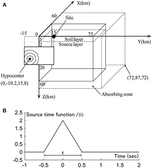
Figure 4. Modeling of ground and fault. (A) Quarter grid model of FDM. (B) Source time function.
In the setting of area source in the three-dimensional FDM, it is necessary to approximate this by multiple point sources placed at the difference grid points. In this paper, multiple point sources are placed at the difference grid points on the source layer and the seismic moment is released by considering the time delay due to the rupture propagation. For this purpose, the fault plane is divided into the small fault size dx = 0.6(km) and small faults of 50 × 30 = 1500 are placed on the source layer. To express the sequential rupture of the divided area sources, it is necessary that dx is sufficiently smaller than the wave length λ(km) of the rupture front. The wave length of the rupture front can be computed by λ = Vr/f = 2.8/1 = 2.8(km) with the effective frequency f = 1(Hz). It can be understood that dx ≪ λ is satisfied and the sequential rupture can be expressed in a sufficient manner.
The following triangle function is employed as the source time function in the fault element.
where fc is the inverse of the rise time τ and τ indicates the width of the bottom of the triangle in f(t). The source time function is shown in Figure 4B.
The three-dimensional difference grid is set as 120km × 150km × 60km (−60km ≤ X ≤ 60km−75km ≤ Y ≤ 75km0km ≤ Z ≤ 60km) as shown in Figure 4A. Figure 4A shows 1/4 of the total region. The material properties of the soil layer and the source layer are shown in Table 1. In the software “GMS,” the inhomogeneous grid is used as the difference grid. The grid interval in the source layer is triple of that in the soil layer. In this paper, the grid interval in the source layer is set so as to satisfy the condition on the effective frequency 0–1 Hz. The fourth-order accurate scheme is used in the difference operator. In the fourth-order accurate scheme, 5–6 grids are required in one wave length (shear wave). In the soil layer, the one grid length 200 (m) leads to the effective frequency f ≤ Vs/(5H) = 2000/(5 × 200) = 2(Hz). On the other hand, in the source layer, the grid length 600(m) leads to the effective frequency f ≤ Vs/(5H) = 3400/(5 × 600) = 1.13(Hz). These parameters satisfy the condition on the effective frequency. The absorbing zone of 12 km is placed at the side and bottom of the object region to damp the reflected wave as shown in Figure 4A. The time duration is 30 (s) and the time increment is 0.015 (s). The number of time steps is 2,000.
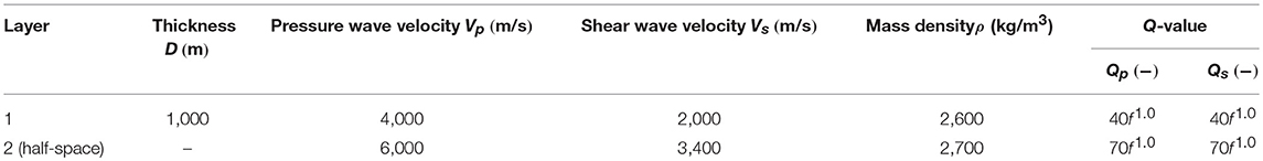
Table 1. Soil conditions.
Consider a 20-story steel building frame. The simplest and most efficient model for vibration analysis of building frames is a shear building model. Usually the shear building modeling is completed by doing a static lateral force analysis for obtaining the story shear-drift relation. However, a shear building model with a predetermined stiffness and strength distribution is assumed here for simple presentation of the proposed critical excitation method. The shear building modeling is conducted and the elastic-plastic response is assumed here. The floor mass is 3.0 × 10⁶ (kg) and the fundamental natural period is 2.4 (s). The story stiffness distribution is assumed to be trapezoidal. The 2% stiffness-proportional structural damping is assumed. The story shear-drift relation is assumed to be bilinear and the yield drift is assumed to be 0.02 (m). The post-yield stiffness ratio to the initial stiffness is 0.05. The target story ductility is 2 and the maximum ductility along height is the objective function.
Although a 20-story steel building frame is treated here for a simple presentation of the proposed excitation method, other types of building structures (reinforced-concrete building structures, taller building structures, etc.) can be dealt with in a similar manner so long as they possess a positive post-yield stiffness. This is because, if building structures with negative post-yield stiffness are treated, the earthquake response may be unstable and the analysis of response sensitivity may cause some difficulties.
In the experimental design planning, CCD, the base point on the axis (Epaxial point) is set to 1.0. The factorial design is planned so that the distances of all the sampling points from the base point are equal. 512 points are prepared in the fractional factorial design. The points of the same number 512 were also added as the sampling points from the uniform random numbers in the hyper sphere.
Consider the following optimization problem by the SQP.
In this paper, the maximum story ductility along height is employed as the objective function h(x). Following Ishii et al. (2000), α = 1.1 and β = 0.95 are assumed. In case of , the maximum value of x is 1.1 and the maximum norm of x is 4.56. The fault model is shown in Figure 5A. Twenty-four control points are chosen and the seismic moment ratios (M0ij, seismic moment at the fault element, , seismic moment of the nominal model at the fault element) at the control points are selected as x. The seismic moments at the control points are varied in this paper.
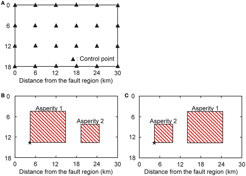
Figure 5. Fault models. (A) Control point for critical model. (B) Recipe model 1. (C) Recipe model 2. *Starting point of fault rupture.
To evaluate the validity of the critical ground motion, two models (Recipe 1 and Recipe 2) are considered based on the strong ground motion prediction recipe (Earthquake Research Committee, 2017). The corresponding fault models are shown in Figures 5B,C. The areas of Asperity 1, Asperity 2, and back ground of the recipe model are , , Sb = 416(km2), respectively. The seismic moments of those are , , . The rise times of those are τa1 = 1.61(sec), τa2 = 1.07(sec),τb = 3.21(sec).
Using the proposed critical excitation method, the critical seismic moment ratios of the critical fault model are obtained. The flowchart of the proposed method is explained in Figure 1 and the detailed explanation is made in section Optimization in Proposed Method.
Figure 6A shows the distribution of critical seismic moment ratios of the critical fault model which produces the maximum story ductility factor. The area ratio of the asperity to the total fault is 22% and the rise time in the asperity is assumed to be τ = 1.95(s). This rise time is slightly longer than that in the recipe model. On the other hand, Figure 6B presents the distribution of asperity. It can be observed from Figure 6B that the asperity with a large area is produced near the observed site and the seismic moment is concentrated at the bottom and left side in the fault. This phenomenon of multiple asperities was seen in the previous work (Makita et al., 2018b).
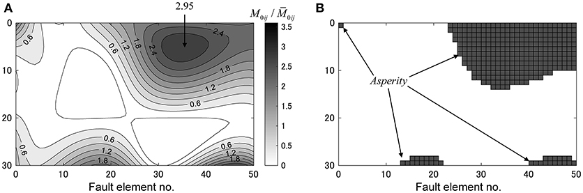
Figure 6. Critical fault model. (A) Distribution of critical seismic moment ratio. (B) Distribution of asperity.
Figure 7 presents the time histories of ground velocity and acceleration (component of transverse) for each fault model. Figure 7A shows the velocities for four models (Recipe model 1, 2, Nominal model, and Critical model). On the other hand, Figure 7B presents the accelerations for such four models. A pulse-type wave can be observed in all fault models. In addition, the maximum velocity and the maximum acceleration were observed in the recipe model 1. Furthermore, the amplitude of the afterward wave is large in the acceleration of Recipe model 2 [(b) in (ii)].
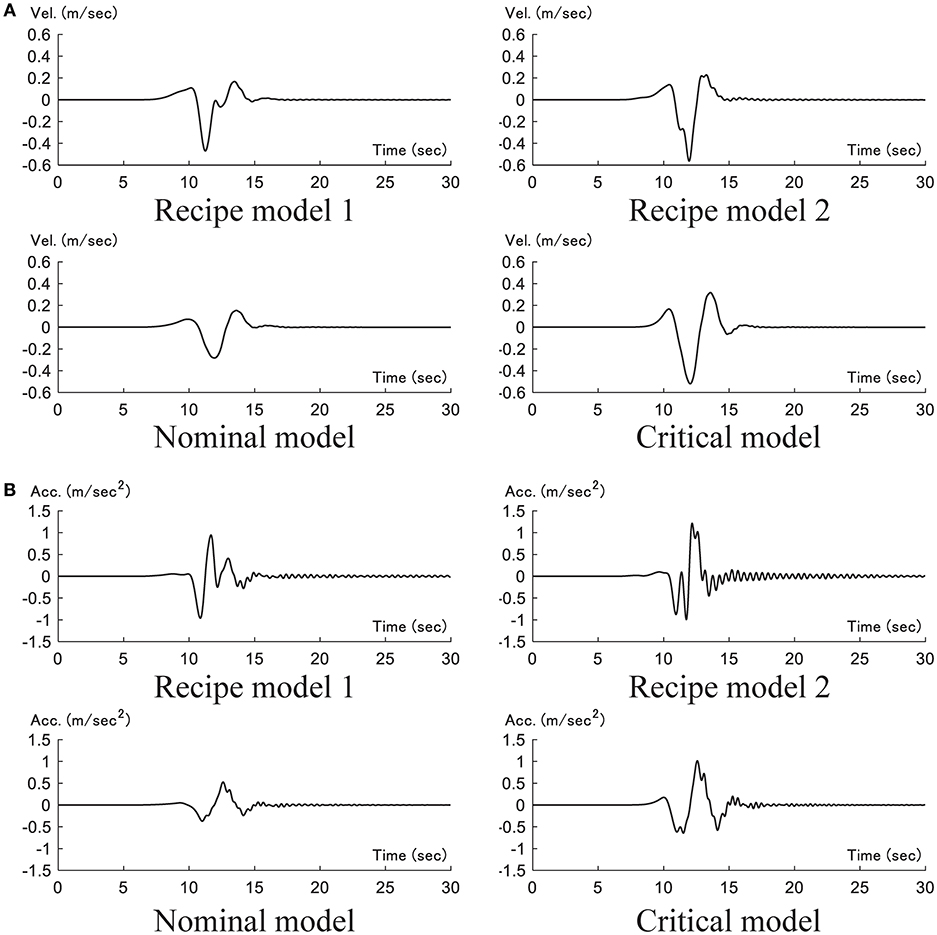
Figure 7. Time history of ground motion (component of transverse) for each fault model. (A) velocity. (B) acceleration.
Figure 8 shows the time histories of inter-story drift and story shear for each fault model (component of transverse). The quantities in 2, 4, 6, 8th stories are presented here. It can be observed that, while the response to the nominal model remains elastic, the responses to Recipe model 1, and the critical model become large and go into the plastic range mainly in the lower stories. The fact whether the building model remains elastic or goes into the plastic range can be found from Figure 9.
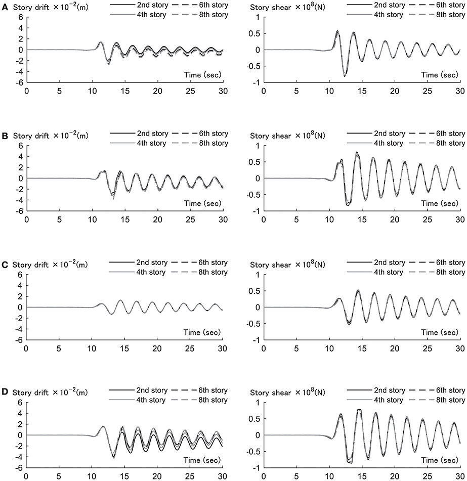
Figure 8. Time history of inter-story drift and story shear for each fault model (component of transverse). (A) Recipe model 1. (B) Recipe model 2. (C) Nominal model. (D) Critical model.
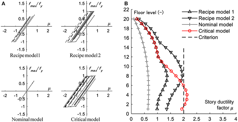
Figure 9. Response for four ground motions. (A) Hysteretic loops in 2, 4, 6, 8th stories for Recipe model 1, 2, Nominal model, and Critical model. (B) Maximum story ductility factors for Recipe model 1, 2, Nominal model, and Critical model.
Figure 9 presents the response for four ground motions. Figure 9A shows the hysteretic loops in 2, 4, 6, 8th stories for Recipe model 1, 2, the Nominal model and the Critical model. It can be observed that the size of the hysteretic loop is large in the order of the Critical model, Recipe model 2, Recipe model 1. Figure 9B illustrates the maximum story ductility factors for Recipe model 1, 2, the Nominal model, and the Critical model. It can be observed that, while the story ductility factors to Recipe model 1, Recipe model 2, and the Nominal model are within the design limit 2, the story ductility factors to the Critical model are beyond the design limit in 2–5th stories. The story ductility factor to the Critical model is 3.2 times larger than that to the Nominal model and 1.1 times larger than that to Recipe model 2.
In this section, the uncertain parameter α in R1 is changed to investigate the influence of the uncertainty level in the fault on the robustness in the response of the superstructure. The concept of the robustness function due to Ben-Haim (2006) is used here.
Figure 10 shows the distribution of seismic moment ratio at each uncertainty level α (1.0–1.5). In the prediction of the fault model, the response surface obtained in the previous analysis is used. The critical fault model for each uncertainty level α (1.0–1.5) is searched via the SQP. This enabled efficient analysis of the robustness function. Focusing on the maximum asperity, the maximum value of is approximately proportional to α up to α = 1.2. On the other hand, when α is larger than 1.3, the maximum value does not change much. This indicates that the proposed method avoids the production of the excessive asperity. In addition, it can be observed that some asperities are located at the edge of the fault except the location near to the observation site.
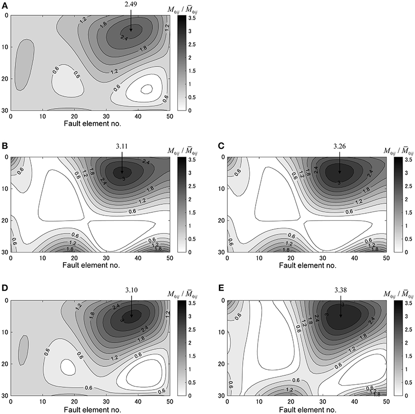
Figure 10. Distribution of seismic moment ratio at each uncertainty level α. (A) α = 1.0. (B) α = 1.2. (C) α = 1.3. (D) α = 1.4. (E) α = 1.5.
Figure 11A shows the maximum value and norm of the control point parameter for various uncertainty levels α . The maximum value is influenced primarily by R1 and the maximum norm is influenced primarily by R2. It can be observed that the maximum value attains the corresponding value α and the maximum norm attain the upper limit of R2 except α = 1.0, 1.4.
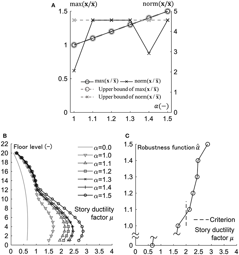
Figure 11. Comparison of responses under several ground motions produced for various uncertainty levels. (A) Maximum value and norm of control point parameter for various uncertainty levels α . (B) Distribution of story ductility factor. (C) Robustness function with respect to story ductility factor.
Figure 11B shows the comparison of ductilities under several ground motions produced for various uncertainty levels. It can be observed that the uncertainty level influences much the responses in the lower stories in this case. Figure 11C presents the robustness function with respect to the ductility (Ben-Haim, 2006). It can be seen that the ductility is over the design criterion (story ductility factor = 2) in the models with the uncertainty level larger than or equal to α = 1.1. This means that the setting of α influences greatly the robustness of the building structure.
In this section, the validity and applicability limit of the proposed method are investigated by comparing with the actual earthquake case. The object earthquake is the Osaka North earthquake in 2018 (MW = 5.67) (Earthquake Research Committee, 2018).
Figure 12A shows the source, observation stations and region of the finite-difference model (GMT). The grid interval is 140 (m). The effective frequency is 0–0.5Hz. The difference grids lower than 30 grids are treated as inhomogeneous ones and the grid interval is made triple. The energy absorbing zone was set at the bottom and the side (60 grids). Figure 12B presents the fault model of this earthquake [(i) Control point for critical model, (ii) Recipe model]. The fault length is 4 km and the fault width is 6 km. The other parameters are strike = 351°, dip = 50°, rake = 52°. The seismic size is (Nm). It is assumed that the fault rupture propagates concentrically from the source with the propagating speed Vr = 2900(m/s). The limit of the uncertainty level is given by α = 1.1 and β = 0.95. The area of asperity, the seismic moment, the rise time are given by , , τa = 0.43(sec),τb = 1.03(sec). Figure 12C shows the comparison between the observation wave and the artificial wave by the recipe model. It can be observed that the frequency content is well simulated at OSK002. However, the amplitude is evaluated in a damped manner. On the other hand, at OSK003, the wave can be simulated well until t = 22 s. However, the amplitude does not correspond well after t = 22 s.
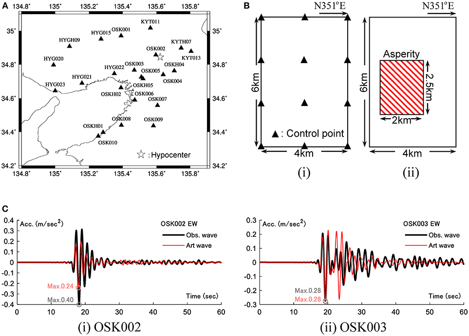
Figure 12. Verification of FDM using 2018 Osaka North earthquake. (A) Source, stations, and region of finite-difference model (GMT). (B) Fault model of 2018 Osaka North earthquake [(i) Control point for critical model, (ii) Recipe model]. (C) Comparison between observation wave and art wave by recipe model.
Figure 13 illustrates the comparison of the box-and-whisker plot of the ratio of displacement response to artificial wave to that to the observation wave between the recipe model (Figure 13A) and the critical model (Figure 13B). It may be concluded that we can produce the critical ground motion under which the displacement response spectrum becomes larger than that under the observed ground motion in the rate of 50% in all natural period ranges and in the rate of 75% in the natural period range up to 13 (s).
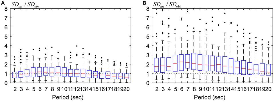
Figure 13. Box-and-whisker plot of ratio of displacement response to art wave to that to observation wave. (A) Recipe model. (B) Critical model.
The finite difference method (FDM)-based critical excitation method has been proposed for building structures with rather long fundamental natural periods. The uncertain parameter is the fault rupture slip distribution described in terms of seismic moments at fault elements. Since the FDM is time-consuming, it is unfavorable to use it in a simple sensitivity algorithm where an independent response sensitivity is calculated for each design parameter (seismic moment at a fault element). To overcome this difficulty, the control points (representative points in the fault) have been introduced. Then the bi-cubic spline interpolation of uncertain parameter distributions (seismic moment distribution) and the response surface method for predicting the response surface from some sampling points have been used effectively. The robustness of building structures for varied uncertainty level of the fault rupture slip (seismic moments in the fault elements) has also been evaluated by using the robustness function. The main conclusions can be summarized as follows.
(1) The introduction of control points in the fault enabled efficient calculation of response sensitivity with respect to change of uncertain parameters (seismic moments in the fault elements). The response surface method also enabled efficient search of the critical distribution of seismic moments in the fault elements.
(2) In addition to the conventional hyper cube variation model, the hyper sphere variation model has been introduced. It was found that the hyper sphere variation model can avoid a drastic change of seismic moments in the fault elements and realistic treatment of uncertainty in the fault is possible.
(3) It was found that the critical ground motion for 20-story building structures with rather long natural period can be found effectively by the proposed method (Figure 9). The maximum ductility under the critical ground motion is 3.2 times larger than that under the ground motion with nominal parameters and 1.1 times larger than that under the ground motion generated by the strong ground motion predicting recipe. As the uncertainty level α in the fault elements becomes larger, the ductility becomes larger linearly approximately (Figure 11).
(4) The fault model of the Osaka North earthquake has been treated as an actual earthquake fault for the investigation of accuracy and reliability of the proposed method. Two kinds of uncertainty modeling, R1 and R2, were used. If we use the setting α = 1.1 and β = 0.95 for R1 and R2, we can produce the critical ground motion under which the response spectrum becomes larger than that under the observed ground motion in the rate of 50% in all natural period ranges and in the rate of 75% in the natural period range up to 13 (s).
KM formulated the problem, conducted the computation, and wrote the paper. KK conducted the computation and discussed the results. IT supervised the research and wrote the paper.
We used the GMS software as the FDM solver and the observation wave of K-NET and KiK-net which were provided by the National Research Institute for Earth Science and Disaster Prevention (NIED). In addition, Figure 12A was generated using the Generic Mapping Tools (Wessel and Smith, 1998). Part of the present work is supported by KAKENHI of Japan Society for the Promotion of Science (No. 17K18922, 18H01584). This support is greatly appreciated.
The authors declare that the research was conducted in the absence of any commercial or financial relationships that could be construed as a potential conflict of interest.
Abrahamson, N., Ashford, S., Elgamal, A., Kramer, S., Seible, F., and Somerville, P. (1998). Proceedings of the 1st PEER Workshop on Characterization of Special Source Effects. CA, Pacific Earthquake Engineering Research Center, University of California, San Diego, CA.
Aoi, S., and Fujiwara, H. (1999). 3-D finite difference method using discontinuous grids. Bull. Seismological Soc. Am. 89, 918–930.
Aoi, S., Honda, R., Morikawa, N., Sekiguchi, H., Suzuki, H., Hayakawa, Y., et al. (2008). Three-dimensional finite difference simulation of long-period ground motions for the 2003 Tokachi-oki, Japan, earthquake. J. Geophys. Res. 113:B07302. doi: 10.1029/2007JB005452
Ben-Haim, Y. (2006). Info-Gap Decision Theory: Decisions Under Severe Uncertainty. 2nd Edn. London: Academic Press.
Bouchon, M. (1981). A simple method to calculate Green's functions for elastic layered media. Bull. Seismol. Soc. Am. 71, 959–971.
Box, G., and Behnken, D. (1960). Some new three level designs for the study of quantitative variables. Technometrics 2, 455–475. doi: 10.1080/00401706.1960.10489912
Cotton, F., Archuleta, R., and Causse, M. (2013). What is sigma of the stress drop? Seismol. Res. Lett. 84, 42–48. doi: 10.1785/0220120087
Day, S. M. (1982). Three-dimensional finite difference simulation of fault dynamics: rectangular fault with fixed rupture velocity. Bull. Seismol. Soc. Am. 72, 83–96.
Drenick, R. F. (1970). Model-free design of aseismic structures. J. Eng. Mech. Division 96, 483–493.
Earthquake Research Committee (2017). Strong Ground Motion Prediction Method for Earthquakes With Specified Source Faults ‘Recipe', The Headquarters for Earthquake Research Promotion. Available online at: https://www.jishin.go.jp/main/chousa/17_yosokuchizu/recipe.pdf
Earthquake Research Committee (2018). Evaluation of June 18, 2018 Osaka North earthquake, The Headquarters for Earthquake Research Promotion. Available online at: https://www.static.jishin.go.jp/resource/monthly/2018/20180618_osaka_2.pdf
Hisada, Y. (2008). Broadband strong motion simulation in layered halfspace using stochastic Green's function technique. J. Seismol. 12, 265–279. doi: 10.1007/s10950-008-9090-6
Hisada, Y., and Bielak, J. (2003). A theoretical method for computing near-fault ground motions in layered half-spaces considering static offset due to surface faulting with a physical interpretation of fling step and rupture directivity. Bull. Seismol. Soc. Am. 93, 1154–1168. doi: 10.1785/0120020165
Irikura, K. (1986). “Prediction of strong acceleration motions using empirical Green's function,” Proc. of the 7th Japan Earthquake Engineering Symposium (Tokyo), 151–156.
Ishii, T., Sato, T., and Somerville, P. G. (2000). Identification of main rupture areas of heterogeneous fault models for strong-motion estimation. J. Struct. Construct. Eng. 527, 61–70. doi: 10.3130/aijs.65.61_1
Khuri, A. I., and Cornell, J. A. (1996). Response Surfaces - Designs and Analysis. New York, NY: Marcel Dekker Inc.
Lawrence Livermore National Laboratory (2002). Guidance for Performing Probabilistic Seismic Hazard Analysis for a Nuclear Plant Site: Example Application to the Southeastern United States. NUREG/CR-6607, UCRL-ID- 133494.
Maeda, T., Iwaki, A., Morikawa, N., Aoi, S., and Fujiwara, H. (2016). Seismic-hazard analysis of long-period ground motion of megathrust earthquakes in the nankai trough based on 3d finite-difference simulation. Seismological Res. Lett. 87, 1265–1273. doi: 10.1785/0220160093
Maeda, T., Morikawa, N., Aoi, S., and Fujiwara, H. (2012). “FD simulation for long-period ground motions of great nankai trough, Japan, earthquakes,” in Proceedings of 15th World Conference on Earthquake Engineering (Lisbon).
Makita, K., Kondo, K., and Takewaki, I. (2018b). Critical ground motion for resilient building design considering uncertainty of fault rupture slip. Front. Built Environ. 4:64. doi: 10.3389/fbuil.2018.00064
Makita, K., Murase, M., Kondo, K., and Takewaki, I. (2018a). Robustness evaluation of base-isolation building-connection hybrid controlled building structures considering uncertainties in deep ground. Front. Built Environ. 4:16. doi: 10.3389/fbuil.2018.00016
Morikawa, N., Kanno, T., Narita, A., Fujiwara, H., Okumura, T., Fukushima, Y., and Guerpinar, A. (2008). Strong motion uncertainty determined from observed records by dense network in Japan. J. Seismol. 12, 529–546. doi: 10.1007/s10950-008-9106-2
Murase, M., Tsuji, M., and Takewaki, I. (2013). Smart passive control of buildings with higher redundancy and robustness using base-isolation and inter-connection. Earthquakes Struct. 4, 649–670. doi: 10.12989/eas.2013.4.6.649
Nickman, A., Hosseini, A., Hamidi, J. H., and Barkhordari, M. A. (2013). Reproducing fling-step and forward directivity at near source site using of multi-objective particle swarm optimization and multi taper. Earthquake Eng. Eng. Vib. 12, 529–540. doi: 10.1007/s11803-013-0194-9
Ohbuchi, M., Itoi, T., and Takada, T. (2011). Reliability-based determination of design earthquake ground motions for performance-based seismic engineering. J. Struct. Construct. Eng. 667, 1583–1589. doi: 10.3130/aijs.76.1583
Okada, T., Fujita, K., and Takewaki, I. (2016). Robustness evaluation of seismic pile response considering uncertainty mechanism of soil properties. Innovat. Infrastruct. Solut. 1:5. doi: 10.1007/s41062-016-0009-8
Somerville, P. G., Irikura, K., Graves, R., Sawada, S., Wald, D., Abrahamson, N., et al. (1999). Characterizing crustal earthquake slip models for the prediction of strong ground motion. Seismological Res. Lett. 70, 59–80 doi: 10.1785/gssrl.70.1.59
Takewaki, I. (2007). Critical Excitation Methods in Earthquake Engineering, 2nd Edn. in 2013. Elsevier.
Tanaka, M., Asano, K., Iwata, T., and Kubo, H. (2014). Source rupture process of the 2011 fukushima-ken hamadori earthquake: how did the two subparallel faults rupture? Earth Planets Space 66:101. doi: 10.1186/1880-5981-66-101
Taniguchi, M., and Takewaki, I. (2015). Bound of earthquake input energy to building structure considering shallow and deep ground uncertainties. Soil Dyn. Earthquake Eng. 77, 267–273. doi: 10.1016/j.soildyn.2015.05.011
Wennerberg, L. (1990). Stochastic summation of empirical Green's functions. Bull. Seismol. Soc. Am. 80, 1418–1432.
Wessel, P., and Smith, W. H. F. (1998). New, improved version of the generic mapping tools released. Eos Trans. AGU 79:579. doi: 10.1029/98EO00426
Yokoi, T., and Irikura, K. (1991). Empirical Green's function technique based on the scaling law of source spectra. J. Seism. Soc. Japan. 44, 109–122.
Yoshimura, C., Bielak, J., Hisada, Y., and Fernandez, A. (2003). Domain reduction method for three-dimensional earthquake modeling in localized regions, Part II: verification and applications. Bull. Seismol. Soc. Am. 93, 825–840. doi: 10.1785/0120010252
Yoshimura, C., Nagano, M., Hisada, Y., Aoi, S., Hayakawa, T., Cital, S. O., et al. (2011). Benchmark tests for strong ground motion prediction methods: case for numerical method (Part1). J. Technol. Design 17, 67–72. doi: 10.3130/aijt.17.67
To investigate the accuracy and reliability of the GMS (software), the comparison with the benchmark test (Yoshimura et al., 2011) has been conducted. Figure A1A shows the fault plane and recording points in the benchmark test. The fault length is 8 km and the fault width is 4 km. The other parameters are strike = 90°, dip = 90°, rake = 180°. The base point is located at (0,0,2)(Km). The seismic size is (Nm). The fault rupture is assumed to propagate concentrically from the source H(Hx, Hy, Hz) = (0, 1, 4)(km) with the propagation speed Vr = 3000(m/s). The number of division of the fault plane is 80 × 40 (3,200). The triangle function was used as the source time function.
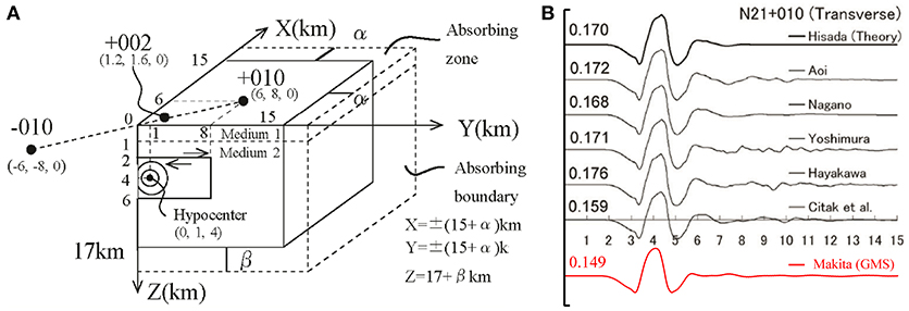
Figure A1. Verification of the present computational method through comparison with benchmark test. (A) Fault plane and recording points (Yoshimura et al., 2011). (B) Comparison between the result due to the GMS and benchmark test (Partly from Yoshimura et al., 2011).
The three-dimensional difference grids are set as 30km × 30km × 17km (−15 km ≤ X ≤ 15 km, −15 km ≤ Y ≤ 15 km, 0 km ≤ Z ≤ 17km) . Figure A1A shows 1/4 of the total model. The material properties of soil layer and source layer are shown in the reference. The effective frequency is 0–1 Hz. Since inhomogeneous grids are used in GMS, the grid interval in the soil layer, and the source layer are 50 m and 150 m, respectively. The absorbing zones are set at the side and bottom of the object region to damp the reflected wave as shown in Figure A1A (60grids). The time duration is 15 (s) and the time increment is 0.005 (s). The number of time steps is 3,000.
Figure A1B presents the comparison (the observation point +010) between the result due to the GMS [designated by “Makita (GMS)”] and the benchmark test. Although the amplitude of the present GMS is slightly smaller than the benchmark test result, the overall velocity wave exhibits a similar property. This indicates the validity of the used software GMS.
Keywords: critical ground motion, worst input, fault rupture, finite difference method (FDM), response surface method, spline interpolation, long-period structure, robustness
Citation: Makita K, Kondo K and Takewaki I (2019) Finite Difference Method-Based Critical Ground Motion and Robustness Evaluation for Long-Period Building Structures Under Uncertainty in Fault Rupture. Front. Built Environ. 5:2. doi: 10.3389/fbuil.2019.00002
Received: 26 November 2018; Accepted: 03 January 2019;
Published: 22 January 2019.
Edited by:
Ehsan Noroozinejad Farsangi, Graduate University of Advanced Technology, IranReviewed by:
Aleksandra Bogdanovic, Institute of Earthquake Engineering and Engineering Seismology, MacedoniaCopyright © 2019 Makita, Kondo and Takewaki. This is an open-access article distributed under the terms of the Creative Commons Attribution License (CC BY). The use, distribution or reproduction in other forums is permitted, provided the original author(s) and the copyright owner(s) are credited and that the original publication in this journal is cited, in accordance with accepted academic practice. No use, distribution or reproduction is permitted which does not comply with these terms.
*Correspondence: Izuru Takewaki, dGFrZXdha2lAYXJjaGkua3lvdG8tdS5hYy5qcA==
Disclaimer: All claims expressed in this article are solely those of the authors and do not necessarily represent those of their affiliated organizations, or those of the publisher, the editors and the reviewers. Any product that may be evaluated in this article or claim that may be made by its manufacturer is not guaranteed or endorsed by the publisher.
Research integrity at Frontiers
Learn more about the work of our research integrity team to safeguard the quality of each article we publish.