 Tsai Yachun1
 Pan Peng
- 1Civil Engineering Department, Tsinghua University, Beijing, China
- 2Key Laboratory of Civil Engineering Safety and Durability of China Education Ministry, Tsinghua University, Beijing, China
Shaking table tests are the most direct experimental way to evaluate structure performance in earthquake engineering. Because of the complexity of the control systems and the influence of specimen behavior, it is difficult for a conventional controller, whose parameters are fixed, to achieve accurate tracking performance for different reference input signals under different payloads. In this paper, a two-loop control method is proposed by combining three-variable control and model reference adaptive control based on Lyapunov stability theory. The proposed control method can adjust the time-domain drive signal adaptively to improve the tracking accuracy and the robustness to specimen uncertainties. Numerical simulations of a small-scale shaking table are used to verify the effectiveness, and the performance of the controller is compared with that of the conventional three-variable control controller. The simulation results demonstrate that the proposed two loop control method provides better performance in both the time and frequency domains.
Introduction
Shaking table tests are the most direct experimental way to evaluate structure performance in earthquake engineering. Typically, a shaking table test system is composed of one or multiple servo-hydraulic actuators, a hydraulic power supply, a rigid table, and a control system. The purpose of the control system of a shaking table is to reproduce reference accelerations that were recorded during an earthquake. However, because of the inherent nonlinearities in hydraulic servo systems and control-structure interaction (CSI) effects, high-fidelity control of a shaking table remains challenging (Dyke et al., 1995; Venanzi et al., 2016; Zhang and Ou, 2016). In the context of shaking table tests, CSI is the coupling of the dynamics of the shaking table with the dynamics of the specimen. The interaction can become more problematic if a specimen changes behavior and its mass is large relative to the mass of the shaking table (Phillips et al., 2014). Hence, a controller that deals with CSI effects is needed.
In addition to the complexity of the shaking table system, the tracking performance of the shaking table in following a specified signal is another challenge. Because acceleration measurements cannot detect constant-velocity motion, direct acceleration feedback control is unstable (Nakata, 2010), and a closed-loop feedback controller is required to stabilize the motion of the shaking table. Traditionally, the hydraulic actuators used in shaking table systems run in a displacement controlled mode, and adopt a proportional-integral-differential (PID) control algorithm. The PID controller can provide reasonable performance in the low-frequency range, but the accuracy of acceleration reproduction is not guaranteed over certain frequency. Thus, the three-variable control (TVC) method was proposed to improve the disadvantages of PID controller. A controller based on TVC consists of feedback and feedforward parts and thus six parameters need to be adjusted. The concept of a TVC controller is to use displacement, velocity and acceleration compensation techniques to improve the dynamics of the shaking table system (Stoten and Shimizu, 2007; Xu et al., 2008; Shen et al., 2011a). Compared to a conventional hydraulic proportional position controller, the TVC controller can enlarge the frequency bandwidth of the acceleration response and increase the system damping ratio. However, the TVC is still a fixed-gain control method, and cannot adjust properly, when the system characteristic of controlled plant changes.
Various control methods for shaking table tests have been proposed to improve the tracking performance of the shaking table. Enokida et al. (2014) introduced a nonlinear signal-based control method(NSBC) to for nonlinear control. NSBC was found to provide the most accurate input identification in all the examined cases of linear or nonlinear single-input, single-output and single-input, multi-output (SIMO) systems. Spencer Jr and Yang (1998) proposed the transfer-function iteration method based on a linearized shaking table model to describe the relationship between the command signal and the measured acceleration. The command signal could be generated beforehand from the desired acceleration by using the inverse model. Twitchell and Symans (2003) used an analytical transfer function for the shaking table dynamics, which was calibrated using a system identification test to simplify offline displacement tracking, and the study demonstrated improved displacement tracking. Phillips et al. (2014) presented a model-based multi-metric control strategy to improve acceleration tracking performance and the susceptibility of the shaking table to specimen dynamics by using both displacement and acceleration measurements. Nakata (2010) developed a method for acceleration trajectory tracking control, which combined an acceleration feedforward controller, displacement feedback, command shaping, and a Kalman filter for the displacement measurement. Stoten (Enokida et al., 2015) applied composite filters to earthquake engineering test systems and prove that composite filters are effective for signal synthesis noise suppression and performance improvement. Yang et al. (2015) proposed a hierarchical control strategy that using sliding mode control to compensate for structural nonlinearities and uncertainties. In recent years there has been a lot of studies for dynamical substructure testing: the hybrid scheme (HS) and the dynamically substructured system (DSS) scheme. Enokida and Stoten (Stoten, 2017a) compared these schemes via test, with a prime focus on the effect of pure time delays. Later, Stoten (2017b) carried out a unification of two methods for controlling dynamically substructured systems. However, the frequency response characteristic of the shaking table system will change with change of payload, and the applicability of the aforementioned methods is limited without consideration being given to the specimen and variation of the payload.
Recently, adaptive control methods have been used to control shaking table systems. Offline iterative control (OIC) requires sufficient data to shape the command signal and reduce the acceleration tracking error. Repetitive excitations may cause premature damage to the specimen (Pipeleers and Swevers, 2010), while the adaptive controller allows online adjustment of its parameters to obtain the desired output. The commonly used ones include minimal control synthesis (MCS) (Stoten and Gómez, 2001; Gizatullin and Edge, 2007; Stoten and Shimizu, 2007; Shen et al., 2011b) adaptive inverse control (AIC) (Salehzadeh-Nobari et al., 1997; Karshenas et al., 2000; Shen et al., 2011a,b; Gang et al., 2013) and self-tuning control (Ghalibafian et al., 2004; Plummer, 2007a,b). Adaptive algorithms achieve high-accuracy performance after the adaptive parameters have converged to the optimal solution. However, they may exhibit poor performance with the initial transient parameters.
This paper proposes a two-loop control method that consists of an inner-loop TVC controller and an outer-loop controller based on model reference adaptive control (MRAC). Compared with the conventional fixed-gain controller (e.g., PID or TVC controller), the two-loop control method can adjust the parameters adaptively during the control process, and has better acceleration performance even when the payload of system changes. The two-loop control method also uses inner-loop controller to deal with the initial transient problem of adaptive algorithm, and the shaking table system achieves high-accuracy performance more quickly. In this paper, open-loop transfer functions are first presented to simulate the uniaxial shaking table system and analyse its stability and controllability. Then, the two-loop control method combining the TVC controller and the MRAC controller is outlined. The TVC controller consists of feedforward and feedback parts, and MRAC controller is based on Lyapunov stability theory. The objective of this combined method is to improve the acceleration output accuracy as well as the robustness to interaction between the shaking table and the specimen. Finally, the effectiveness of the proposed strategy is verified by shaking table tests with different payloads, particularly for cases in which the mass of the specimen is relatively large compared to that of the table.
System Modeling
The shaking table is driven by the hydraulic system shown in Figure 1, which includes a servo valve, a hydraulic actuator and a power supply. The connections among those subsystems make the dynamics of the hydraulic actuators complex and nonlinear. A mathematical model of the physical system can be obtained from De Silva (1988); Conte and Trombetti (2000); Plummer (2007a,b); Shen et al. (2012). In this section, we derive the dynamics and interactions among the components in the hydraulic shaking table system.
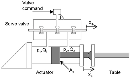
Figure 1. Schematic of hydraulic systems.
Hydraulic Actuator Modeling
The command to the valve controls the position of the valve spool that regulates the oil flux to the actuator chambers and drives the hydraulic actuator. First, we formulate a relationship between the valve command to the servo valve and the oil flux to the actuator chambers. Equation (1) is an empirical linear model of the valve dynamics in terms of a second-order lag plus a delay:
where xq is the valve spool displacement, uq is the valve command, ζq and ωq are the damping ratio and natural frequency of the servo valve, respectively, τ is the time delay and s is a Laplace variable.
The linearized oil flux QL which is defined as QL = (Q1 + Q2)/ 2, can be expressed as
where kq is the gain of the servo valve and pL = p1 − p2 is the pressure drop across the actuator chambers. The term KC is the flow pressure coefficient, which can be expressed as
where Cd is the discharge coefficient, w is the constant area gradient of the servo valve orifice, ρ is the mass density of the fluid and pS is the hydraulic supply pressure.
Using the flow continuity equation, the oil flux, which is the driving source of the hydraulic actuator, can be obtained as
where Ap is the effective piston area, xa is the actuator displacement, Va is the volume of the actuator chambers, β is the bulk modulus of the hydraulic fluid and s is a Laplace variable. The term Ctc is the total leakage coefficient of the actuator, which comprises the internal leakage coefficient Cip and the external leakage coefficient Cep, and is defined as Ctc = Cip + Cep/2. Equation (4) shows that the oil flux is influenced by the piston movement, the chamber volume change and the oil leakage. A block diagram of the hydraulic actuator system is shown in Figure 2.
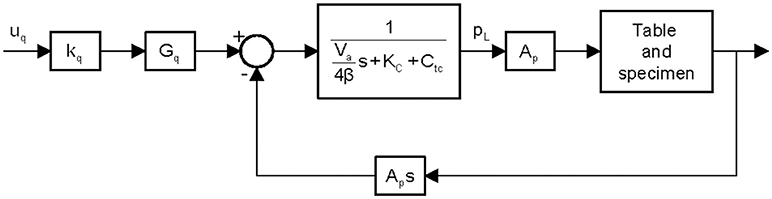
Figure 2. Block diagram of hydraulic systems.
Governing Equation of Table Motion
A simplified unidirectional shaking table system, which consists of a rigid table and a specimen with a single degree of freedom, is shown in Figure 3. Here, dt is the relative displacement of the shaking table with respect to the ground, ds is the relative displacement of the specimen with respect to the table, mt and ms are the masses of the shaking table and the specimen, respectively, and Fa represents the force of the actuator. To maintain the centring capacity of the table, the shaking table is connected to a reaction wall by a linear spring whose stiffness is k. The equation of motion can be written as
where csand ks are the damping and elastic stiffness of the specimen, respectively. Equations (5) and (6) can be transformed into Equaion (7), which can be expressed as the state-space representation shown in Equation (8):
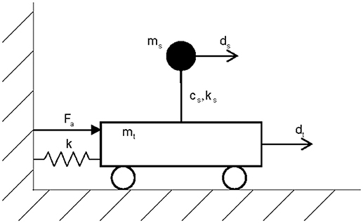
Figure 3. Schematic of single-degree-of-freedom shake-table system.
Two-Loop Control Method
An innovative two-loop control method combining the MRAC and TVC is proposed for uniaxial shaking table tests. The block diagram of the two-loop control method is shown in Figure 4. In the figure, um(t) is the reference signal, us(t) is the MRAC signal, u(t) is the control signal of the controlled plant, xs(t) and xm(t) are the state vectors of the outputs of the controlled plant and reference model, respectively, Kp and Ku are the adaptive gains and ex(t) is the state error.
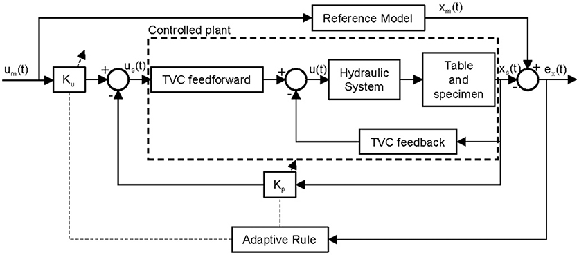
Figure 4. Block diagram of proposed control Strategy.
As shown in Figure 4, the two-loop control method uses an inner-loop controller and an outer-loop controller based on TVC and MRAC, respectively. The two-loop control method uses MRAC for the outer loop instead of OIC to reduce the tracking error and avoid causing premature damage to the specimen. The MRAC controller can adjust its parameters online to improve the robustness of the system dynamics. The two-loop control method also uses TVC for the inner loop to accelerate convergence of the adaptive algorithm. This is because the initial variation of the adaptive gains is often accompanied by poor transient response if only MRAC is adopted. In addition, using a TVC controller can enlarge the frequency bandwidth and improve the stability of the control system (Xu et al., 2008; Gang et al., 2013). In the two-loop control method, only the table and the specimen are modeled and the others, e.g., the hydraulic system and the TVC controller, are not included in reference model, so that the movement of the table is identical with the input ground motions. Furthermore, the reference model is designed for a specimen whose mass is small relative to that of the shaking table to minimize interaction with the specimen dynamics, whereas a real controlled plant may have a specimen with a large mass. The adaptive rule is expected to ensure that the controlled plant tracks the response of the reference model even if the specimen mass differs between the reference model and the controlled plant.
Three-Variable Controller Design
The TVC controller is commonly used to generate the earthquake excitations of shaking tables (Tagawa and Kajiwara, 2007). Block diagrams of the reference signal generator and the TVC controller are shown in (Figures 5A,B), respectively. As shown in Figure 5A, the reference signal generator uses the reference acceleration signal to generate the reference states. These mainly include the reference displacement, velocity and acceleration, which are denoted by rd, ṙd and , respectively (Gang et al., 2013). The transfer function of the signal generator can be expressed as
where Kg is the acceleration gain, ξ0 is the damping ratio of the acceleration control, ω0 is the natural frequency of the acceleration and d0 and v0 are the integral constants for rd and ṙd, respectively. In TVC, d0 and v0 are commonly taken to be and 2ξ0ω0, respectively.
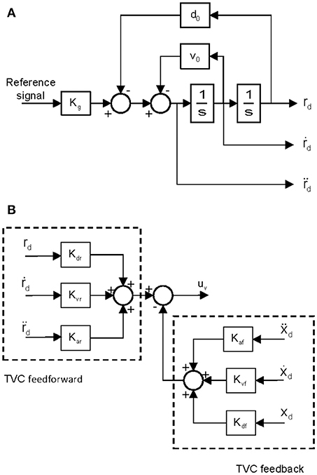
Figure 5. Three-variable controller. (A) Block diagrams of the reference signal generator. (B) Block diagrams of TVC controller.
As shown in Figure 5B, the TVC can be separated into a feedforward controller and a feedback controller. Terms xd, ẋd and ẍd are the measured displacement, velocity and acceleration, respectively, and uv is the TVC output. The feedback part can improve the control stability by means of feedback loops whose feedback gains are Kdf, Kvf, and Kaf for displacement, velocity and acceleration, respectively. The feedforward part can extend the acceleration frequency and improve the reference tracking accuracy by adjusting the feedforward gains Kdr, Kvr, and Kar, which are gains for displacement, velocity and acceleration, respectively, in the feedforward loop. Note that the TVC controller is an inner-loop controller that is in the control chain of the MRAC controller. The signal is first processed by the outer-loop MRAC controller, and then passed to the TVC controller.
Model Reference Adaptive Controller Design
Based on Lyapunov stability theory, MRAC was originally proposed in the 1960s (Parks, 1966; Landau, 1984). The method involves creating a closed-loop controller that works on the principle of adjusting the controller parameters by measuring the difference between the outputs of the controlled plant and the reference model, so that the controlled plant can follow the behavior of the reference model. In this study, MRAC based on Lyapunov stability theory is applied to improve the accuracy of tracking and robustness against CSI. A shaking table system with a small loading specimen is used for the reference model; its output is tracked by the controlled plant, which can be a shaking table system with a large loading specimen.
The governing equations of the controlled plant including the TVC controller and the shaking table system are
where xs(t) is the state vector of the table and specimen as defined in Equation (7), us(t) is the adaptive control input signal, ys(t) is the output vector of the table and specimen for the controlled plant, As is the 4 × 4 state matrix of the controlled plant, Bs is its 4 × 1 input matrix, and Cs is its 2 × 4 output matrix.
The governing equations of the reference model are
where xm(t) is the state vector of the reference model, um(t) is the reference input signal, which is commonly a reference acceleration time-history record, ym(t) is the output vector of the table and specimen for the reference model, Am is the 4 × 4 state matrix of the reference model, Bm is its 4 × 1 input matrix (as defined in Equation 8) and Cs is its 2 × 4 output matrix. The output matrices Cm and Cs are
In this study, the output vectors take only the displacement and velocity of the table into account.
The tracking error and state error are denoted by ey(t) and ex(t), respectively:
The MRAC signal is defined as
where Kp[ex(t), t] and Ku[ex(t), t] are time-variant gainmatrices. Substituting Equation (15) into Equation (10), we obtain
Then, we assume that and exist and satisfy
where and are the corresponding parameters for the MRAC input signal when the state vector of the controlled plant matches that of the reference model exactly.
In this paper, we use Lyapunov stability theory to design the MRAC. Substituting Equations (10, 11, 15, 17) into Equation (14) yields
where and are the error signals of the controller parameters and are defined as
From Lyapunov stability theory, the state matrix of the reference model Am is the Hurwitz matrix; in other words, Am is asymptotically stable. Thus, there exists a symmetric positive-definite solution P to Equation (20) for any choice of symmetric positive-definite matrix Q:
We consider a positive-definite quadratic Lyapunov candidate function that contains the state error vector and the error signal of the controller parameters, namely
where and are symmetric positive-definite constant matrices with appropriate dimensions.
The derivative of the Lyapunov candidate function and the details of the associated proof procedure are given in the Appendix. Because V(t) is positive definite and is negative definite, Lyapunov stability theory guarantees that ex(t) will approach zero asymptotically and that the tracking error ey(t) will also vanish asymptotically. The adaptive gains can be designed as
Numerical Simulations
A small-scale electro-hydraulic shaking table was selected to verify the effectiveness of the proposed controller, namely MRAC combined with TVC. As shown in Figure 3, the simplified unidirectional shaking table system consists of a rigid table and a specimen with a single degree of freedom. The mass of the shaking table was 6,000 kg. Four different loading specimens, two with relatively small mass and two with relatively large mass compared with the mass of the shaking table, were used in the numerical simulations to investigate the CSI effects. The performance of the two-loop controller combining MRAC and TVC is assessed by comparing the table motion and the input earthquake ground motion.
The simulation evaluation analysis was performed in MATLAB/Simulink. The parameters for the hydraulic actuator model, the shaking table system and the TVC controller gains used in the simulations are listed in Table 1. In this study, the specimen was assumed to be linearly elastic. Its mass for the MRAC reference model was taken to be 6 kg (i.e., 1/1000 the table mass) to minimize any interaction due to the dynamics of the specimen. The state matrices of the reference model were obtained using Equation (11), and those of the controlled plant were determined from Equation (10) once the payload was chosen. The symmetric positive-definite matrix P was obtained from Equation (20), and the adaptive gains Kp[ex(t), t] and Ku[ex(t), t] were obtained from Equation (22).
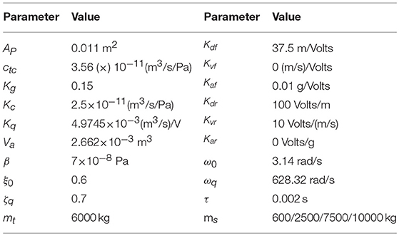
Table 1. Main parameters of shaking table system.
The TVC is commonly used in shaking table test, and it can improve the stability of the control system. In this study, a conventional TVC control method was implemented for the purpose of comparison. The parameters of for the MRAC controller were optimized by using the genetic algorithm. For the optimization, we adopted the bare-table case, in which the mass of the specimen is zero, subjected to a synthesized ground motion NAcc1 (refer to Table 2), and the parameters were optimized by minimizing the RMS of tracking error of acceleration in time domain. The optimized parameters were used for all the cases with different specimen masses. Note that the parameters remaining unchanged for TVC, whereas they served only as initial values and kept updating for MRAC.
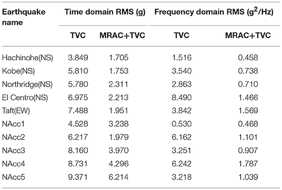
Table 2. RMS of acceleration error for a payload of 10,000 kg in time and frequency domains.
The mass of the specimen is first considered as 7,500 kg, and the ground motions recorded during the Northridge and Taft earthquakes are taken as the reference signals. Figures 6, 7 show the simulation results for Northridge and Taft, respectively. As shown in Figures 6A,B, both controllers are able to track the reference acceleration in general. However, comparing the curves shown in Figures 6C,D reveals that MRAC combined with TVC achieves much better accuracy. Figure 7 shows the comparison in the frequency domain. Both controllers perform well at frequencies lower than 6 Hz but the two-loop control combining MRAC and TVC has better performance, particularly at medium and high frequencies. We conclude that the proposed control strategy offers better performance for acceleration control in both the time and frequency domains.
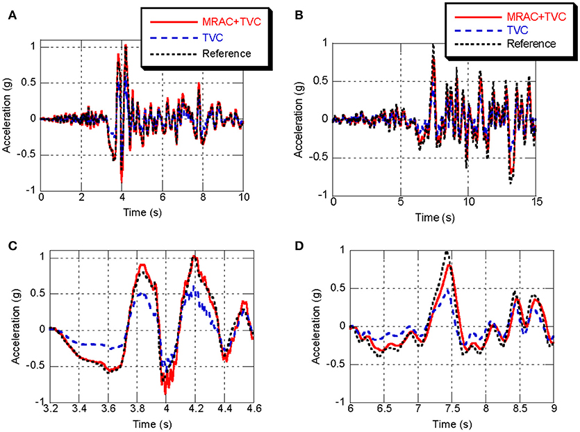
Figure 6. Comparison of table performance in time domain. (A,C) Wide and narrow views of acceleration tracking for the Northridge earthquake. (B,D) Wide and narrow views of acceleration tracking for the Taft earthquake.
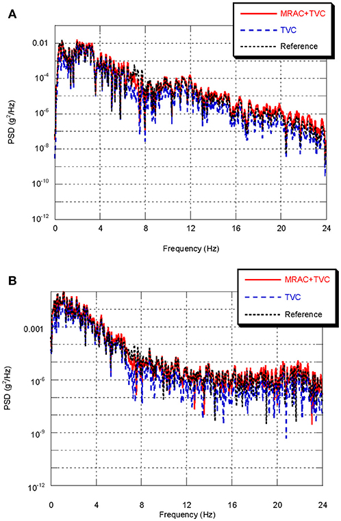
Figure 7. Comparison of table performance in frequency domain. Acceleration power spectral density for (A) Northridge earthquake and (B) Taft earthquake.
Next, we consider five cases in which the mass of the specimen is zero, 600, 2,500, 7,500, and 10,000 kg. Simulations for the five cases were carried out using 10 instances of ground motion. Detailed simulation results for the case with a specimen mass of 10,000 kg are given in Table 2. There, the root mean square (RMS) of the tracking error between the reference and measured table motions is compared between the conventional control method and the proposed one in both the time and frequency domains. Note that the RMS of the tracking error is normalized against the maximum absolute value of the reference acceleration record. In the time domain, it can be observed that the tracking errors for the proposed control method are all smaller than those obtained from the conventional control method.
Table 3 compares the median and standard deviation of the errors between the conventional control method and the proposed one for the five cases in both the time and frequency domains. From Table 3, it can be found that the tracking errors increase with the increase of the specimen mass, demonstrating that the CSI effects cannot be neglected. In all cases, the median value and standard deviation of the acceleration tracking errors of the proposed control method are smaller than those of the conventional control method. In addition, comparing the RMS of the bare-table case with that of the case with the maximum payload, it increased by roughly 15% under the TVC, which adopts fixed gains, whereas it increases by only roughly 7% under MRAC. The results show that the proposed controller performs much better than the conventional TVC controller, not only improving the accuracy of the shaking table system but also providing good robustness against CSI effects and specimen uncertainties.
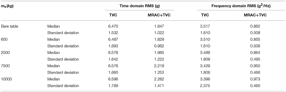
Table 3. Median and standard deviation of RMS.
Equations (15) and (22) indicate that Kp[ex(t), t] and Ku[ex(t), t] adjust their values according to the variation of the entire state error. In this study, the output vectors take the displacement and velocity of the shaking table into account. Furthermore, the MRAC parameters are designated as Kp[ey(t), t] and Ku[ey(t), t], which are two-dimensional and one-dimensional vectors, respectively:
Figures 8, 9 show the adjustment of Kp[ey(t), t] and Ku[ey(t), t] for the proposed control method. The specimen mass is 7,500 kg and the ground motions recorded during the Northridge and Taft earthquakes are taken as the reference signals. From both figures, it can be observed that the values of Kp[ey(t), t] and Ku[ey(t), t] vary with time during the simulation process, and gradually become stable when the output difference between the controlled plant and the reference model becomes smaller.
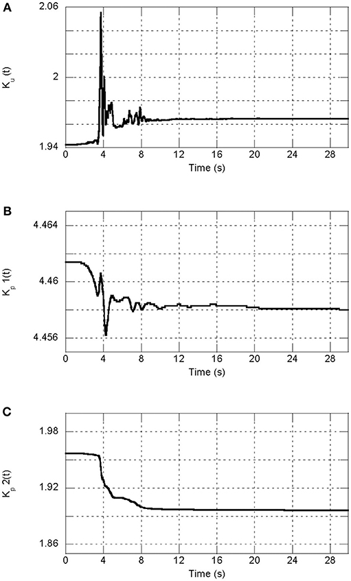
Figure 8. Adjustment of MRAC controller parameters for the Northridge earthquake. (A) Adjustment of Ku[ey(t), t]. (B,C) Adjustment of Kp[ey(t), t].
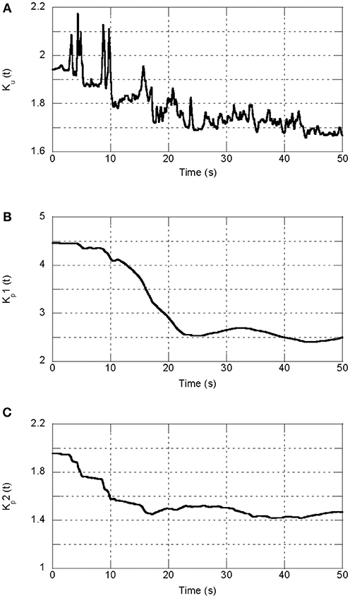
Figure 9. Adjustment of MRAC controller parameters for the Taft earthquake. (A) Adjustment of Ku[ey(t), t]. (B,C) Adjustment of Kp[ey(t), t].
The adaptive algorithm achieves high-accuracy performance after the adaptive parameters have converged to the optimal solution, but it may exhibit poor performance in the beginning if it adopts inappropriate initial parameters. In this study, the TVC controller is used as an inner-loop controller, not only to improve the stability of the shaking table system but also to deal with the initial transients. Figure 10 shows a comparison of tracking error convergence during the simulation process between the proposed control method and the MRAC-only controller. The tracking error was investigated using the same specimen and ground motion, namely 7,500 kg and the Northridge earthquake, respectively. As shown in Figure 10, either with or without the TVC controller, satisfactory performance is achieved with high control accuracy after the adaptive algorithm converges. However, the tracking error with the proposed strategy is even smaller than that with the MRAC controller and takes only half the time to converge. Thus, it can be concluded that using the inner-loop TVC controller improves the initial poor transient response of MRAC and converges to the optimal solution more quickly.
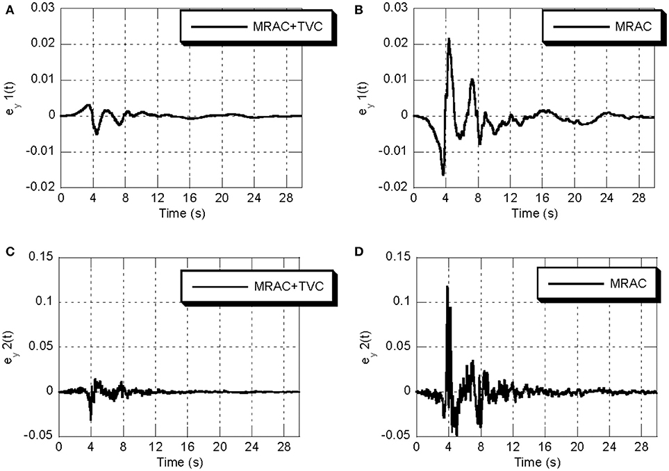
Figure 10. Comparison of tracking error convergence of adaptive algorithm for the Northridge earthquake. (A,C) Using combined strategy. (B,D) Using only MRAC.
Conclusions
An innovative two-loop control method consisting of an inner-loop TVC controller and an outer-loop MRAC controller was proposed to improve the acceleration tracking performance of a shaking table. An adaptive MRAC rule was developed based on Lyapunov stability theory. The proposed control method was applied to a small-scale shaking table for different payloads in numerical simulations. The conventional TVC controller was used for comparison to verify the effectiveness. A MRAC controller was also used for comparison to show that the inner-loop TVC controller could deal with the problem of the initial transients of the adaptive algorithm. The major conclusions obtained from this study are as follows.
(1) Compared with the conventional fixed-gain controller (e.g., TVC controller), the two-loop control method can adjust the parameters adaptively during the control process, and has better performance for acceleration control in both the time and frequency domains.
(2) For different payloads, the RMS of the tracking errors under two-loop control is consistently smaller than that obtained from the conventional control method. This shows that the proposed method has good robustness against specimen uncertainties and CSI effects.
(3) Compared with the MRAC method, the adaptive algorithm in the two-loop control method takes half the time to converge to the optimal solution. Hence, the controlled plant achieves high-accuracy performance more quickly.
(4) Accurate information about the controlled plant is not required for the two-loop control method. Furthermore, the shaking table system will follow the desired reference signal without causing premature damage to the specimen.
Author Contributions
TY and PP proposed the conception of work. TY, ZD, and ZY developed the two-loop control method and carried out the numerical simulation of shaking table. TY and ZD analyzed the uniaxial shaking table system. PP, TY, ZD and ZY wrote the manuscript.
Conflict of Interest Statement
The authors declare that the research was conducted in the absence of any commercial or financial relationships that could be construed as a potential conflict of interest.
Acknowledgments
Financial supports from the Natural Science Foundation of China [grant numbers 51422809 and 51578314], the Beijing Science and Technology Program [grant number Z161100001216015] and the Tsinghua University Initiative Scientific Research Program [grant number 2014Z22067], are gratefully acknowledged.
References
Conte, J., and Trombetti, T. (2000). Linear dynamic modeling of a uni-axial servo-hydraulic shaking table system. Earthq. Eng. Struct. Dyn. 29, 1375–1404. doi: 10.1002/1096-9845(200009)29:9<1375::AID-EQE975>3.0.CO;2-3
Dyke, S., Spencer Jr B. F., Quast, P., and Sain, M. K., (1995). Role of control-structure interaction in protective system design. J. Eng. Mech. 121, 322–338. doi: 10.1061/(ASCE)0733-9399(1995)121:2(322)
Enokida, R., Stoten, D., and Kajiwara, K. (2015). Stability analysis and comparative experimentation for two substructuring schemes, with a pure time delay in the actuation system. J. Sound Vib. 346, 1–16. doi: 10.1016/j.jsv.2015.02.024
Enokida, R., Takewaki, I., and Stoten, D. (2014). A nonlinear signal-based control method and its applications to input identification for nonlinear SIMO problems. J. Sound Vib. 333, 6607–6622. doi: 10.1016/j.jsv.2014.07.014
Gang, S., Zhen-Cai, Z., Lei, Z., Yu, T., Chi-fu, Y., Jin-Song, Z., et al. (2013). Adaptive feed-forward compensation for hybrid control with acceleration time waveform replication on electro-hydraulic shaking table. Control Eng. Pract. 21, 1128–1142. doi: 10.1016/j.conengprac.2013.03.007
Ghalibafian, H., Bhuyan, G. S., Ventura, C., Rainer, J.H., Borthwick, D., Stewart, R.P., et al. (2004). Seismic behaviour of flexible conductors connecting substation equipment-Part II: shake table tests. IEEE Trans. Power Deliv. 19, 1680–1687. doi: 10.1109/TPWRD.2004.832387
Gizatullin, A., and Edge, K. (2007). Adaptive control for a multi-axis hydraulic test rig. Proc. Instit. Mech. Eng. Part I 221, 183–198. doi: 10.1243/09596518JSCE314
Karshenas, M., Dunnigan, M., and Williams, B. (2000). Adaptive inverse control algorithm for shock testing. IEE Proc. Control Theory Appl. 147, 267–276. doi: 10.1049/ip-cta:20000166
Landau, Y. D. (1984). Adaptive control: the model reference approach. IEEE Trans. Syst. Man Cybern. 169–170. doi: 10.1109/TSMC.1984.6313284
Nakata, N. (2010). Acceleration trajectory tracking control for earthquake simulators. Eng. Struct. 32, 2229–2236. doi: 10.1016/j.engstruct.2010.03.025
Parks, P. (1966). Liapunov redesign of model reference adaptive control systems. IEEE Trans. Automat. Contr. 11, 362–367. doi: 10.1109/TAC.1966.1098361
Phillips, B. M., Wierschem, N. E., and Spencer, B. (2014). Model-based multi-metric control of uniaxial shake tables. Earthq. Eng. Struct. Dyn. 43, 681–699. doi: 10.1002/eqe.2366
Pipeleers, G., and Swevers, J. (2010). Optimal feedforward controller design for periodic inputs. Int. J. Control 83, 1044–1053. doi: 10.1080/00207170903552067
Plummer, A. (2007a). Robust electrohydraulic force control. Proc. Instit. Mech. Eng. Part I 221, 717–731. doi: 10.1243/09596518JSCE370
Plummer, A. (2007b). Control techniques for structural testing: a review. Proc. Instit. Mech. Eng. Part I 221, 139–169. doi: 10.1243/09596518JSCE295
Salehzadeh-Nobari, S., Chambers, J. A., Green, T. C., Goodfellow, J. K., and Smith, W. E. D. (1997). “Implementation of frequency domain adaptive control in vibration test products,” in Fifth International Conference on Factory 2000 - The Technology Exploitation Process (Cambridge, UK).
Shen, G., Lv, G. M., Ye, Z. M., Cong, D. C., and Han, J. W. (2011b). Implementation of electrohydraulic shaking table controllers with a combined adaptive inverse control and minimal control synthesis algorithm. IET control theory applications, 5, 1471–1483. doi: 10.1049/iet-cta.2010.0198
Shen, G., Lv, G. M., Ye, Z. M., Cong, D. C., and Han, J. W. (2012). Feed-forward inverse control for transient waveform replication on electro-hydraulic shaking table. J. Vib. Control 18, 1474–1493. doi: 10.1177/1077546311417743
Shen, G., Zheng, S. T., Ye, Z. M., Yang, Z. D., Zhao, Y., Han, J. W., et al. (2011a). Tracking control of an electro-hydraulic shaking table system using a combined feedforward inverse model and adaptive inverse control for real-time testing. Proc. Instit. Mech. Eng. Part I 225, 647–666. doi: 10.1177/2041304110394529
Spencer, Jr, B., and Yang, G. (1998). “Earthquake simulator control by transfer function iteration,” in Proceedings of the 12th ASCE Engineering Mechanics Conference (La Jolla, CA).
Stoten, D., and Shimizu, N. (2007). The feedforward minimal control synthesis algorithm and its application to the control of shaking-tables. Proc. Instit. Mech. Eng. Part I 221, 423–444. doi: 10.1243/09596518JSCE246
Stoten, D. P. (2017a). A comparative study and unification of two methods for controlling dynamically substructured systems. Earthq. Eng. Struct. Dyn. 46, 317–339. doi: 10.1002/eqe.2797
Stoten, D. P. (2017b). Generalised formulation of composite filters and their application to earthquake engineering test systems. Earthq. Eng. Struct. Dyn. 46, 2619–2635. doi: 10.1002/eqe.2921
Stoten, D. P., and Gómez, E. G. (2001). Adaptive control of shaking tables using the minimal control synthesis algorithm. Philos. Trans. R. Soc. London A 359, 1697–1723. doi: 10.1098/rsta.2001.0862
Tagawa, Y., and Kajiwara, K. (2007). Controller development for the E-Defense shaking table. Proc. Instit. Mech. Eng. Part I 221, 171–181. doi: 10.1243/09596518JSCE331
Twitchell, B. S., and Symans, M. D. (2003). Analytical modeling, system identification, and tracking performance of uniaxial seismic simulators. J. Eng. Mech. 129, 1485–1488. doi: 10.1061/(ASCE)0733-9399(2003)129:12(1485)
Venanzi, I., Ierimonti, L., and Ubertini, F. (2016). Effects of control-structure interaction in active mass driver systems with electric torsional servomotor for seismic applications. Bull. Earthq. Eng. 15, 1543–1557. doi: 10.1007/s10518-016-0021-6
Xu, Y., Hua, H., and Han, J. (2008). Modeling and controller design of a shaking table in an active structural control system. Mech. Syst. Signal Process. 22, 1917–1923. doi: 10.1016/j.ymssp.2008.02.003
Yang, T., Li, K., Lin, J. Y., Li, Y., and Tung, D. P. (2015). Development of high-performance shake tables using the hierarchical control strategy and nonlinear control techniques. Earthq. Eng. Struct. Dyn. 44, 1717–1728. doi: 10.1002/eqe.2551
Zhang, C., and Ou, J. (2016). Control structure interaction of electromagnetic mass damper system for structural vibration control. J. Eng. Mech. 134, 428–437. doi: 10.1061/(ASCE)0733-9399(2008)134:5(428)
Appendix
Taking the derivative of the positive-definite quadratic Lyapunov candidate function of Equation (21) gives
Substituting Equations (18, 20) into Equation (A1), can be expressed as
Because every term in Equation (A2) is a real number, and using
we can obtain
If and are defined as
then
Because V(t) is positive definite and is negative definite, Lyapunov stability theory guarantees that the entire state error ex(t) will approach 0 asymptotically, and that the tracking error ey(t) will vanish asymptotically. By Equations (19) and (A5), the adaptive gains can be designed as
Keywords: adaptive control, model reference adaptive control, lyapunov stability theory, three-variable control, hydraulic actuator, shaking table test
Citation: Yachun T, Peng P, Dongbin Z and Yi Z (2018) A Two-Loop Control Method for Shaking Table Tests Combining Model Reference Adaptive Control and Three-Variable Control. Front. Built Environ. 4:54. doi: 10.3389/fbuil.2018.00054
Received: 20 June 2018; Accepted: 21 September 2018;
Published: 16 October 2018.
Edited by:
Tomaso Trombetti, Università degli Studi di Bologna, ItalyCopyright © 2018 Yachun, Peng, Dongbin and Yi. This is an open-access article distributed under the terms of the Creative Commons Attribution License (CC BY). The use, distribution or reproduction in other forums is permitted, provided the original author(s) and the copyright owner(s) are credited and that the original publication in this journal is cited, in accordance with accepted academic practice. No use, distribution or reproduction is permitted which does not comply with these terms.
*Correspondence: Pan Peng, cGFucGVuZ0BtYWlsLnRzaW5naHVhLmVkdS5jbg==