Gaussian Process Time-Series Models for Structures under Operational Variability

A wide range of vibrating structures are characterized by variable structural dynamics resulting from changes in environmental and operational conditions, posing challenges in their identification and associated condition assessment. To tackle this issue, the present contribution introduces a stochastic modeling methodology via Gaussian Process (GP) time-series models. In the presently introduced approach, the vibration response is represented by means of a random coefficient time-series model, whose coefficients comply with a GP regression on the environmental and operational parameters. The approach may be implemented in conjunction to any type of linear-in-the-parameters time-series model, ranging from simple AR models to more complex non-linear or non-stationary time-series models. The obtained GP time-series modeling approach provides an effective and compact global representation of the vibrational response of a structure under a wide span of environmental and operational conditions. The effectiveness of the postulated GP time-series models is demonstrated through two case studies: the first involves the identification of the vertical vibration response of the Humber bridge, evaluated over a period of three years; the second considers the long-term simulated vibration response of a wind turbine featuring non-stationary dynamics stemming from the rotor speed. In both cases, the variation of the average wind speed is the main driver of uncertainty, while, through application of the proposed GP time-series models, it is possible to track the resulting variation in modal quantities.

1. Introduction

Several types of vibrating structures by default operate in constantly varying environmental and operational conditions, which inevitably results in variability of the induced structural dynamics. This is the case for wind turbines, bridges, high rise buildings and more. This issue poses a practical challenge related to the identification and analysis of the vibrational response of these structures, as well as for the health monitoring, fatigue assessment and control of the induced vibrations.

In order to construct a robust model of the dynamic response of the structure, it is not only necessary to accurately model the short-term response of the structure, but it is further necessary to effectively capture the long-term trends underlying the induced dynamics. This issue, in the particular case of data-based time-series models, has been extensively researched in recent years, resulting in the formulation of different strategies, including projection methods, and deterministic or stochastic functional dependence models. Projection methods, also referred to as data normalization methods, aim at projecting characteristic quantities associated with the time-series model representing the short-term response of the structure, into a subspace where the influence of Environmental and Operational Parameters (EOPs) may be easily removed (Yan et al., 2005; Sohn, 2007; Deraemaeker et al., 2008). On the other hand, deterministic functional dependence models aim at capturing the long-term variability in the dynamics by assuming a deterministic functional relationship from EOPs to the characteristic quantities of the time-series model describing the dynamics of the response. Typically, such a deterministic functional relationship is captured via a functional series expansion. Methods falling into this class include the regression/interpolation methods discussed in Worden et al. (2002) and Sohn (2007), as well as the Functionally Pooled (FP) time-series models explained in Kopsaftopoulos et al. (2018) and Sakellariou and Fassois (2016). These methods are particularly effective when a direct relationship exists between measurable input EOPs and the characteristic quantities of the time-series models. Nonetheless, uncertainty in the EOPs and in the dynamic response introduces variability in the characteristic quantities of the basic time-series model, which may not be effectively captured by means of a deterministic relationship. Instead, random or stochastic functions may be more effective in capturing the uncertainty on the characteristic quantities of the time-series model.

In this sense, a third class of methods, referred to as stochastic functional dependence models, aim at capturing the long-term variability by assuming that the characteristic quantities of the basic time-series model are stochastic variables depending on the EOPs. Toward this end, recent works have postulated either Random Coefficient (RC) (Avendaño-Valencia and Fassois, 2015, 2017a,b; Avendaño-Valencia et al., 2015a) or Polynomial Chaos Expansions (PCE) (Spiridonakos and Chatzi, 2014, 2015; Avendaño-Valencia et al., 2015b; Spiridonakos et al., 2016) to represent the variability of the characteristic quantities of a model. In particular, RC time-series models represent the variability in the dynamics as randomness in the parameters of the time-series model. Then, apart from the selection of the specific time-series model, a further user-defined choice pertains to the definition of an appropriate distribution model for its respective coefficients, which in several cases can become very complex. On the other hand the PCE approach exploits the probabilistic knowledge of the EOPs to build the most effective functional representation of the time-series parameters. However, it is also considered that the randomness in the model parameters originates solely on the randomness of the EOPs. Therefore, other sources of uncertainty may be misrepresented.

In this regard, this work provides a framework for the global (short and long term) identification of the dynamic response of a structure, of unknown properties or a given a priori numerical model, under variable operational and environmental conditions by representing the short-term dynamics via a linear-in-the parameters regressive time-series model (which may assume the form of an AutoRegressive, AutoRegressive with eXogenous input or similar model), and a Gaussian Process (GP) regression to represent the stochastic dependence of the parameters of the basic time-series model on the EOPs, which in turn, describes the long-term variability on the dynamics of the structural response. Contrary to deterministic functional dependence models and PCE-based methods, where the EOPs are considered as the sole source of variability on the time-series model parameters, the appraised GP approach is further capable of capturing and quantifying the additional uncertainty stemming from other unmeasurable sources. Likewise, the obtained GP time-series model is totally linear-in-the-parameters, which facilitates the identification, parameter estimation and posterior model-based analysis. The issue of model identification is addressed by the Maximum Likelihood principle, which is solved by means of an Expectation-Maximization method adapted to the particular structure of the Gaussian Process time-series model. In addition, Gaussian Process Principal Component Regression (GP-PCR) is introduced as an optional improvement to the basic GP time-series model aiming at reducing the number of variables in the representation and to improve the numerical stability of the parameter estimation and optimization.

The methods discussed here are demonstrated on two dedicated case-studies. The first one pertains to the identification of actual data corresponding to the vertical acceleration response in the Humber bridge measured over 21 non-consecutive days in the period from May 19, 2011, to March 24, 2013. The second one corresponds to the identification of the long-term vibration response of a wind turbine, employing simulations obtained via the FAST wind turbine aeroelastic simulation code, which are characterized by non-stationary dynamics and long-term variability induced by variable wind speed.

The remainder of this paper is organized as follows: Section 2 initially provides a summary of traditional linear-in-the-parameters time-series models, pointing out their limitations in long-term identification, and offering their natural extension via GP regression. In addition, principal component regression is introduced as an alternative to reduce the number of identified parameters. Subsequently, Section 3 is devoted to the identification of the GP time-series model based on a set of dynamic responses, including the estimation of the parameters of individual realizations, the estimation of the hyper-parameters of the representation and the assessment and validation of the obtained model. Finally, Section 4 provides the two aforementioned case studies, i.e., the Humber bridge and wind turbine simulated vibrational response, while Section 5 concludes the study.

2. Models of the Dynamic Response of Structures

2.1. Traditional Linear-in-the-Parameters Regressive Time-Series Models

Consider the dynamic response of a structure y[t] ∈ ℝ defined over the normalized discrete time t = 1, 2, …, N and sampled with a sampling rate f_s. The response is assumed to obey the linear-in-the-parameters regressive time-series model:

$y\left[t\right]={\mathit{\varphi }}^T\left(\mathit{z}\left[t\right]\right)\cdot \mathit{\theta }+w\left[t\right],w\left[t\right]\sim \mathtt{\text{NID}}\left(0,{\mathrm{\sigma }}_w^2\right)$ (1)

where ϕ (z [t]) ∈ ℝⁿ is the regression vector, $\mathit{z}\left[t\right]\in {\mathbb{R}}^{n_z}$ is the vector of regressed variables, $\mathit{\theta }\in \mathbb{R}$ⁿ is the parameter vector and w[t] is a Normally and Identically Distributed (NID) innovations of mean zero and variance ${\mathrm{\sigma }}_w^2$. The vector of regressed variables z [t] may contain previous values of the dynamic response y[t], excitation inputs $\mathit{x}\left[t\right]$ and innovations w[t], according to the model type. Accordingly, equation (1) corresponds to the case of either an output-only or a Multiple Input Single Output (MISO) model. However, the Multiple Input Multiple Output (MIMO) case can be cast into the presently discussed framework through the proper rearrangement of the regression and parameter vectors, as well as the redefinition of the dynamic response and innovations as column vectors. In addition, linear state space representations may be considered when observation errors are an important component of the dynamic response measurements.

The linear-in-the-parameters regressive time-series model of equation (1) encompasses a large group of time-series models, which differ in the specific form of the regression vector and the vector of regressed variables. A few important examples are summarized next:

• AutoRegressive (AR) models: the simplest case corresponds to the AR model, for which the regression vector is of the form ((Ljung, 1999) Ch. 4):

$\mathit{\varphi }\left(\mathit{z}\left[t\right]\right)=\mathit{z}\left[t\right]={\left[\begin{array}{cccc}\hfill y\left[t-1\right]\hfill & \hfill y\left[t-2\right]\hfill & \hfill \cdots \hfill & \hfill y\left[t-n_a\right]\hfill \end{array}\right]}^T$ (2)

where n_a is the order of the AR model.

• AutoRegressive Moving Average (ARMA) models: ARMA models further include previous values of the innovations in the vector of regressed variables, and thus (Ljung, 1999):

$\mathit{\varphi }\left(\mathit{z}\left[t\right]\right)=\mathit{z}\left[t\right]={\left[\begin{array}{cccccc}\hfill y\left[t-1\right]\hfill & \hfill \cdots \hfill & \hfill y\left[t-n_a\right]\hfill & \hfill w\left[t-1\right]\hfill & \hfill \cdots \hfill & \hfill w\left[t-n_c\right]\hfill \end{array}\right]}^T$ (3)

where n_a and n_c are the orders of the AR and MA parts of the model.

• AutoRegressive with eXogenous variable (ARX) models: ARX models combine previous values of the dynamic response and the excitation vector $\mathit{x}\left[t\right]\in {\mathbb{R}}^{n_x}$, and thus ((Ljung, 1999) Ch. 4):

$\mathit{\varphi }\left(\mathit{z}\left[t\right]\right)=\mathit{z}\left[t\right]={\left[\begin{array}{cccccc}\hfill y\left[t-1\right]\hfill & \hfill \cdots \hfill & \hfill y\left[t-n_a\right]\hfill & \hfill {\mathit{x}}^T\left[t-1\right]\hfill & \hfill \cdots \hfill & \hfill {\mathit{x}}^T\left[t-n_b\right]\hfill \end{array}\right]}^T$ (4)

where n_a and n_b are the orders of the AR and exogenous parts of the model.

• Linear Parameter Varying AR (LPV-AR) models: LPV-AR models are a class of time-dependent AR models, which correspond to a generalization of the simple AR model, where the parameters of the AR model are dependent on an external scheduling variable β[t] determining the values of these parameters at time t. The regression vector in the case of LPV-AR models is of the form (Avendaño-Valencia and Fassois, 2017b):

$\mathit{z}\left[t\right]={\left[\begin{array}{cccc}\hfill y\left[t-1\right]\hfill & \hfill y\left[t-2\right]\hfill & \hfill \cdots \hfill & \hfill y\left[t-n_a\right]\hfill \end{array}\right]}^T$ (5a)

$\mathit{\varphi }\left(\mathit{z}\left[t\right]\right)=\mathit{z}\left[t\right]\otimes {\left[\begin{array}{cccc}\hfill g_{b_1}\left(\mathrm{\beta }\left[t\right]\right)\hfill & \hfill g_{b_2}\left(\mathrm{\beta }\left[t\right]\right)\hfill & \hfill \cdots \hfill & \hfill g_{b_p}\left(\mathrm{\beta }\left[t\right]\right)\hfill \end{array}\right]}^T$ (5b)

where n_a is the AR order, ⊗ denotes the Kronecker product, $g_{b_j}\left(\mathrm{\beta }\left[t\right]\right)$ is the j-th functional expansion basis, and p is the order of the functional expansion basis. The closely related Functional Series TAR (FS-TAR) models form a special case of the LPV-AR model where the scheduling variable is time, i.e., β[t] ≡ t (Poulimenos and Fassois, 2006).

• Non-linear AR (NAR) models: NAR models correspond to the non-linear counterpart of AR models, where the dynamic response is regressed on non-linear functions of its previous values, so that the regression vector assumes the form (Spiridonakos and Chatzi, 2015):

$\mathit{\text{z}}\left[t\right]={\left[\begin{array}{cccc}\hfill y\left[t-1\right]\hfill & \hfill y\left[t-2\right]\hfill & \hfill \cdots \hfill & \hfill y\left[t-n_a\right]\hfill \end{array}\right]}^T$ (6a)

$\mathit{\varphi }\left(\mathit{z}\left[t\right]\right)={\left[\begin{array}{cccc}\hfill g_1\left(\mathit{z}\left[t\right]\right)\hfill & \hfill g_2\left(\mathit{z}\left[t\right]\right)\hfill & \hfill \cdots \hfill & \hfill g_n\left(\mathit{z}\left[t\right]\right)\hfill \end{array}\right]}^T$ (6b)

where n_a is the AR order, and g_j (z [t]) is the j–th non-linear term of the vector of regressed variables.

Equation (1) may be expressed alternatively as follows:

$w\left[t\right]=y\left[t\right]-{\mathit{\varphi }}^T\left(\mathit{\text{z}}\left[t\right]\right)\cdot \mathit{\theta }=y\left[t\right]-y\left[t|t-1\right]$ (7)

where y[t|t – 1]: = E{y[t]|θ, ϕ (z [t])} is the one-step-ahead prediction of the dynamic response, with associated variance $E\left\{\left(y\left[t_1\right]-y\left[t_1|t_1-1\right]\right)\cdot \left(y\left[t_2\right]-y\left[t_2|t_2-1\right]\right)\right\}={\mathrm{\sigma }}_w^2\cdot \mathrm{\delta }\left[t_1-t_2\right]$, where t₁, t₂ are two analysis instants, and δ[t] denotes the Kronecker delta. Hence, under the NID assumption of the innovations w[t], the conditional probability of the dynamic response y[t] given the parameter vector θ and the regression vector ϕ (z [t]) is Gaussian with mean y[t|t–1] and variance ${\mathrm{\sigma }}_w^2$, or more specifically:

$p\left(y\left[t\right]|\mathit{\theta },\mathit{\varphi }\left(\mathit{z}\left[t\right]\right)\right)={\mathcal{N}}_{y\left[t\right]}\left(y\left[t|t-1\right],{\mathrm{\sigma }}_w^2\right),y\left[t|t-1\right]={\mathit{\varphi }}^T\left(\mathit{z}\left[t\right]\right)\cdot \mathit{\theta }$ (8)

where ${\mathcal{N}}_x\left(x_o,{\mathrm{\sigma }}_x^2\right)$ denotes a Gaussian distribution for the random variable x with mean x_o and variance ${\mathrm{\sigma }}_x^2$. Moreover, by virtue of the NID nature of the innovations, it follows that the probability for an entire vibration response realization of length N aggregated in the vector y = [y[1] y[2] ⋅ ⋅ ⋅ y[N]]^T, is:

$p\left(\mathit{y}|\mathit{\theta },\mathbf{\Phi }\right)={\displaystyle \prod _{t=1}^N}p\left(y\left[t\right]|\mathit{\theta },\mathit{\varphi }\left(\mathit{z}\left[t\right]\right)\right)={\displaystyle \prod _{t=1}^N}{\mathcal{N}}_{y\left[t\right]}\left(y\left[t|t-1\right],{\mathrm{\sigma }}_w^2\right)$ (9)

where Φ = [ϕ (z [1]) ϕ (z [2]) ⋯ ϕ (z [N])] ∈ ℝ^{n × N} is the N-sample long regression matrix. Then, by introduction of equation 8, and by virtue of the properties of exponential functions, it follows that (see Appendix A.1):

$p\left(\mathit{y}|\mathit{\theta },\mathbf{\Phi }\right)={\mathcal{N}}_y\left({\mathbf{\Phi }}^T\cdot \mathit{\theta },{\mathrm{\sigma }}_w^2\cdot {\mathit{I}}_N\right)$ (10)

where I_N indicates the N-size identity matrix. The conditional PDF p(y |θ, Φ), seen as a function of the parameter vector θ, determines the likelihood of the parameter vector ℒ(θ | y, Φ). Furthermore, after assuming that the coefficient vector θ is a deterministic variable, Maximum Likelihood (ML) estimates may be obtained by determining the values that maximize the likelihood ℒ(θ | y, Φ) ((Ljung, 1999), Sec. 7.4).

2.2. Limitations of the Traditional Linear Regressive Models

Although the linear-in-the-parameters regressive time-series model shown in equation (1) is useful for representing diverse classes of time-series, including stationary, non-stationary and non-linear, it lacks the flexibility to effectively represent variable dynamics stemming from variable Environmental and Operational Conditions (EOCs). For instance, it is known that the elasticity modulus of a material may change with temperature, and in turn, a change in this variable would modify the natural frequencies and damping ratios associated with the dynamic response of the structure. Hence, the model in equation (1) with a fixed parameter vector θ, would fail to effectively represent the dynamic response of the structure over a long period of analysis.

Instead, it may be considered that during a given period of time, say T = N ⋅ f_s, the EOCs remain more or less constant, and consequently, the physical parameters of the structure would also remain constant. Under these conditions, the linear regression model of equation (1) is a valid representation of the dynamic response of the structure for such analysis period, while the parameter vector θ would change according to the EOCs. Two main questions may be identified in this regard, the first is on how to select the length of the period where it is considered that the structural parameters remain more or less constant; the second is on how to represent the variability in the parameters as a function of the EOCs. The selection of the period of pseudoconstant dynamics may be obtained empirically by means of stationarity tests, as described for example in Kay (2008), Basu et al. (2009), and Borgnat et al. (2010). On the other hand, the representation of the variability in the dynamics of the structure as an effect of the EOCs is the main problem addressed in this work, for which a Gaussian Process Regression approach is postulated, as shown in the remainder of this work.

2.3. Gaussian Process Time-Series Model

The key assumption in the Gaussian Process (GP) regression approach is that the parameter vector of the time-series model follows a Gaussian distribution. Therefore, the linear-in-the-parameters regressive time-series model of equation (1), is complemented as follows:

$y\left[t\right]={\mathit{\varphi }}^T\left(z\left[t\right]\right)\cdot \mathit{\theta }+w\left[t\right],w\left[t\right]\sim \mathtt{\text{NID}}\left(0,{\mathrm{\sigma }}_w^2\right)$ (11a)

$\mathit{\theta }={\mathit{\theta }}_o\left(\mathit{\xi },\mathit{M}\right)+\mathit{u},\mathit{u}\sim \mathtt{\text{NID}}\left({\mathbf{\text{0}}}_{n\times 1},{\mathbf{\Sigma }}_{\mathrm{\theta }}\right)$ (11b)

where ξ ∈ ℝ^m is the Environmental and Operational Parameter (EOP) vector determining the EOCs in the analysis period, θ₀(ξ, M) = E{θ |ξ, M} is the mean parameter vector indicating the expected value of the parameter vector given the EOP ξ and the matrix of projection coefficients M ∈ ℝ^{n × p}, and u is an NID random vector with mean zero and covariance Σ_θ. The model is completed by the following functional series expansion of the mean parameter vector:

${\mathit{\theta }}_o\left(\mathit{\xi },\mathit{M}\right)={\displaystyle \sum _{j=1}^p}{\mathit{\mu }}_j\cdot g_{b_j}\left(\mathit{\xi }\right)=\mathit{M}\cdot \mathit{g}\left(\mathit{\xi }\right)$ (12)

where p is the order of the functional series expansion and:

$\mathit{M}=\left[\begin{array}{ccc}\hfill {\mathit{\mu }}_1\hfill & \hfill \cdots \hfill & \hfill {\mathit{\mu }}_p\hfill \end{array}\right]\in {\mathbb{R}}^{n\times p}\mathit{g}\left(\mathit{\xi }\right)=\left[\begin{array}{c}\hfill g_{b_1}\left(\mathit{\xi }\right)\hfill \\ \hfill ⋮\hfill \\ \hfill g_{b_p}\left(\mathit{\xi }\right)\hfill \end{array}\right]\in {\mathbb{R}}^{p\times 1}$ (13)

are the matrix of projection coefficients and the functional basis vector containing the basis with indices $\mathit{b}={\left[\begin{array}{ccc}\hfill b_1\hfill & \hfill \cdots \hfill & \hfill b_p\hfill \end{array}\right]}_{p\times 1}^T$, b_j ∈ ℕ. Note that any type of non-linear function may have been used to describe the parameter variation, however, a linear-in-the-parameter structure has been selected—again—in equation (12) to facilitate the estimation and analysis of the model. A time-series model obeying equation (11) shall be referred to as a Gaussian Process (GP) time-series model and is characterized by a set of deterministic parameters, referred to as hyper-parameters $\mathcal{P}=\left\{\mathit{M},{\mathbf{\Sigma }}_{\mathit{\theta }},{\mathrm{\sigma }}_w^2\right\}$, consisting of the matrix of projection coefficients, the parameter covariance matrix and the innovations variance.

For a GP time-series model, the instantaneous value of the dynamic response y[t] and the parameter vector θ are jointly distributed Gaussian variables, with the joint PDF conditioned on the regression vector, the EOP vector and the hyper-parameters shown next:

$p\left(y\left[t\right],\mathit{\theta }|\mathit{\varphi }\left[t\right],\mathit{\xi },\mathcal{P}\right)=p\left(y\left[t\right]|\mathit{\varphi }\left[t\right],\mathit{\theta },\mathit{\xi },\mathcal{P}\right)\cdot p\left(\mathit{\theta }|\mathit{\varphi }\left[t\right],\mathit{\xi },\mathcal{P}\right)$ (14)

where, from equation (11), it follows that:

$p\left(y\left[t\right]|\mathit{\theta },\mathit{\varphi }\left[t\right],\mathit{\xi },\mathcal{P}\right)={\mathcal{N}}_{y\left[t\right]}\left(y\left[t|t-1\right],{\mathrm{\sigma }}_w^2\right)$ (15a)

$p\left(\mathit{\theta }|\mathit{\varphi }\left[t\right],\mathit{\xi },\mathcal{P}\right)={\mathcal{N}}_{\mathit{\theta }}\left({\mathit{\theta }}_o\left(\mathit{\xi },\mathcal{M}\right),{\mathbf{\Sigma }}_{\mathit{\theta }}\right)$ (15b)

Similarly, when the dynamic response over the complete period of analysis of length N, namely y, is considered, the respective joint conditional PDF takes the form:

$p\left(\mathit{y},\mathit{\theta }|\mathbf{\Phi },\mathit{\xi },\mathcal{P}\right)={\displaystyle \prod _{t=1}^N}p\left(y\left[t\right],\mathit{\theta }|\mathit{\varphi }\left[t\right],\mathit{\xi },\mathcal{P}\right)={\displaystyle \prod _{t=1}^N}p\left(y\left[t\right]|\mathit{\theta },\mathit{\varphi }\left[t\right],\mathit{\xi },\mathcal{P}\right)\cdot p\left(\mathit{\theta }|\mathit{\varphi }\left[t\right],\mathit{\xi },\mathcal{P}\right)$ (16)

which, under the Gaussianity of both p(y[t]|θ, ϕ [t], ξ, 𝒫) and p(θ |ϕ [t], ξ, 𝒫), becomes:

$p\left(\mathit{y},\mathit{\theta }|\mathbf{\Phi },\mathit{\xi },\mathcal{P}\right)=\underset{\mathit{p}\left(y|\mathit{\theta },\mathbf{\Phi },\mathit{\xi },\mathcal{P}\right)}{\underbrace{{\mathcal{N}}_y\left({\mathbf{\Phi }}^T\cdot \mathit{\theta },{\mathrm{\sigma }}_w^2\cdot {\mathit{I}}_N\right)}}\cdot \underset{p\left(\mathit{\theta }|\mathbf{\Phi },\mathit{\xi },\mathcal{P}\right)}{\underbrace{{\mathcal{N}}_{\mathit{\theta }}\left({\mathit{\theta }}_o\left(\mathit{\xi },\mathit{M}\right),N^{-1}\cdot {\mathbf{\Sigma }}_{\mathit{\theta }}\right)}}$ (17)

In addition, according to the conditional density axiom, the joint PDF may be decomposed as follows ((Rasmussen and Williams, 2006), p. 9):

$p\left(\mathit{y},\mathit{\theta }|\mathbf{\Phi },\mathit{\xi },\mathcal{P}\right)=p\left(y|\mathit{\theta },\mathbf{\Phi },\mathit{\xi },\mathcal{P}\right)\cdot p\left(\mathit{\theta }|\mathbf{\Phi },\mathit{\xi },\mathcal{P}\right)=p\left(\mathit{\theta }|y,\mathbf{\Phi },\mathit{\xi },\mathcal{P}\right)\cdot p\left(\mathit{y}|\mathbf{\Phi },\mathit{\xi },\mathcal{P}\right)$ (18)

where $p\left(\mathit{\theta }\text{|}\mathit{y},\mathbf{\Phi },\mathit{\xi },\mathcal{P}\right)$ is the posterior PDF of the parameter vector after observing the dynamic response, and p(y | Φ, ξ, 𝒫) is the marginal probability of the dynamic response, comprising a function of the hyper–parameters and is referred to as the marginal likelihood of the hyper-parameters ℒ(𝒫 | y, Φ, ξ). The latter is obtained by marginalizing the joint conditional PDF p(y, θ |Φ, ξ, 𝒫) with respect to all the possible values of θ (Rasmussen and Williams, 2006), p. 9). Given that both distributions p(y | θ, Φ, ξ, 𝒫) and p(θ |Φ, ξ, 𝒫) are Gaussian, the posterior parameter PDF and marginal likelihood are Gaussian as well, of the form (Rasmussen and Williams, 2006), p. 9):

$p\left(\mathit{\theta }|\mathit{y},\mathbf{\Phi },\mathit{\xi },\mathcal{P}\right)={\mathcal{N}}_{\mathit{\theta }}\left(\widehat{\mathit{\theta }},P_{\mathit{\theta }}\right)$ (19a)

$\mathcal{L}\left(\mathcal{P}|\mathit{y},\mathbf{\Phi },\mathit{\xi }\right)=p\left(\mathit{y}|\mathbf{\Phi },\mathit{\xi },\mathcal{P}\right)={\mathcal{N}}_{\mathit{\text{y}}}\left({\mathbf{\Phi }}^T\cdot {\mathit{\theta }}_o\left(\mathit{\xi },M\right),{\Sigma }_{{\mathrm{\epsilon }}_k}\right)$ (19b)

where

$\widehat{\mathit{\theta }}=\mathtt{\text{E}}\left\{\mathit{\theta }|\mathit{y},\mathbf{\Phi },\mathit{\xi },\mathcal{P}\right\}={\mathit{\theta }}_o\left(\mathit{\xi },\mathit{M}\right)+\mathit{K}\cdot \left(\mathit{y}-{\mathbf{\Phi }}^T\cdot {\mathit{\theta }}_o\left(\mathit{\xi },\mathit{M}\right)\right)$ (20a)

${\mathit{P}}_{\mathit{\theta }}=\mathtt{\text{E}}\left\{\left(\mathit{\theta }-\widehat{\mathit{\theta }}\right)\cdot {\left(\mathit{\theta }-\widehat{\mathit{\theta }}\right)}^T\mathrm{|}\mathit{y},\mathbf{\Phi },\mathit{\xi },\mathcal{P}\right\}=\left({\mathit{I}}_n-\mathit{K}\cdot {\mathbf{\Phi }}^T\right)\cdot {\mathbf{\Sigma }}_{\mathit{\theta }}$ (20b)

$\mathit{K}={\mathbf{\Sigma }}_{\mathit{\theta }}\cdot \mathbf{\Phi }\cdot {\mathbf{\Sigma }}_{\mathrm{\epsilon }}^{-1}$ (20c)

${\mathbf{\Sigma }}_{\mathrm{\epsilon }}={\mathrm{\sigma }}_w^2\cdot {\mathit{I}}_N+{\mathbf{\Phi }}^T\cdot {\mathbf{\Sigma }}_{\mathit{\theta }}\cdot \mathbf{\Phi }$ (20d)

In the previous equations $\widehat{\mathit{\theta }}\in {\mathbb{R}}^n$ corresponds to the posterior parameter mean with the associated posterior parameter covariance matrix P_θ ∈ ℝ^{n × n}. Moreover, the quantities:

$\tilde{y}\left[t|t-1\right]:={\mathit{\varphi }}^T\left(\mathit{z}\left[t\right]\right)\cdot {\mathit{\theta }}_o\left(\mathit{\xi },\mathit{M}\right),\mathrm{\epsilon }\left[t\right]:=y\left[t\right]-\tilde{y}\left[t|t-1\right]$ (21a)

$y\left[t|t-1\right]:={\mathit{\varphi }}^T\left(\mathit{z}\left[t\right]\right)\cdot \widehat{\mathit{\theta }},e\left[t\right]:=y\left[t\right]-y\left[t|t-1\right]$ (21b)

are referred to as the prior and posterior one-step-ahead predictions, respectively, with associated prior and posterior prediction errors ε[t] and e[t]. In addition, Σ_ε ∈ ℝ^{N × N} is the covariance matrix of the prior prediction error. The main difference between the prior and posterior predictions, is that the prior predictions correspond to the best guess of the dynamic response in the absence of knowledge of the actual parameter vector at the period of analysis, while the posterior predictions are the best guess of the dynamic response based on (an estimate of) the actual parameter vector.

2.3.1. Remark – Unknown or Non-Measurable Sources of Uncertainty

The GP time-series model may also be used in the context where the EOP vector is either unknown or unmeasurable. If that is the case, the functional series expansion of the mean parameter vector in equation (12) is limited to a single constant term, so that θ₀(ξ, M): = θ₀ = μ₁⋅1, while the parameter PDF reduces to the conventional multivariate Gaussian model, so that $\mathit{\theta }\sim \mathcal{N}$_θ (θ₀, Σ_θ). Such a case has been explored in Avendaño-Valencia et al. (2015a).

2.4. Regression on a Reduced Parameter Set via Principal Component Regression

A potential difficulty in the adoption of the GP time-series models lies in the computational cost due to the large number of parameters that need to be estimated. Moreover, a coefficient vector covariance matrix Σ_θ with full structure implies that several of the estimated parameters are redundant and/or unnecessary. A potential solution to this problem is to use a dimensionality reduction scheme for the regression matrix, such as in Principal Component Regression (PCR), which is explained next.

To start with, consider the matrix ${\overline{\mathbf{\Phi }}}_K={\left[{\mathbf{\Phi }}_1{\mathbf{\Phi }}_2\cdots {\mathbf{\Phi }}_K\right]}^T\in {\mathbb{R}}^{n\times \left(N\cdot K\right)}$ containing the regression matrices associated with the set of dynamic responses 𝒴_K, which possesses the Singular Value Decomposition (SVD) $\overline{\mathbf{\Phi }}=\mathit{\text{U}}\cdot \mathbf{\Lambda }\cdot {\mathit{\text{V}}}^T$, where U ∈ ℝ^{n × m} and V ∈ ℝ^{(N⋅K) × m} are orthogonal matrices, and Λ ∈ ℝ^{m × m}, with m = min{(N ⋅ K – 1), n} designating the rank of ${\overline{\mathbf{\Phi }}}_K$, is a diagonal singular value matrix with entries λ₁ ≥ λ₂ ≥ ⋯ ≥ λ_m. Moreover, consider the vector $\mathit{d}={\left[\begin{array}{cccc}\hfill d_1\hfill & \hfill d_2\hfill & \hfill \cdots \hfill & \hfill d_{\tilde{m}}\hfill \end{array}\right]}^T$ of dimension $\tilde{m}\le m$ containing the indices of selected singular values, and the truncated eigenvector matrices $\tilde{\mathit{U}}\in {\mathbb{R}}^{n\times \tilde{m}}$ and $\tilde{\mathit{V}}\in {\mathbb{R}}^{\left(N\cdot K\right)\times \tilde{m}}$ built from the columns of U and V corresponding to the indices in d.

Hence, if the regression vector ϕ (z [t]) is projected into the column Eigen-space, so that:

$\tilde{\mathit{U}}\cdot \tilde{\mathit{\varphi }}\left(\mathit{z}\left[t\right]\right)=\mathit{\varphi }\left(\mathit{z}\left[t\right]\right)\leftrightarrow \tilde{\mathit{\varphi }}\left(\mathit{z}\left[t\right]\right)={\tilde{\mathit{U}}}^T\cdot \mathit{\varphi }\left(\mathit{z}\left[t\right]\right)$ (22)

Then, upon replacement of the previous result into the original regression model, the alternative Principal Component Gaussian Process Regression (PC-GP) time-series model is obtained:

$y\left[t\right]={\tilde{\mathit{\varphi }}}^T\left(\mathit{z}\left[t\right]\right)\cdot \mathrm{\vartheta }+w\left[t\right],w\left[t\right]\sim \mathtt{\text{NID}}\left(0,{\mathrm{\sigma }}_w^2\right)$ (23a)

$\mathit{\vartheta }={\mathit{\vartheta }}_o\left(\mathit{\xi },\tilde{M}\right)+\tilde{\mathit{u}},\tilde{\mathit{u}}\sim \mathtt{\text{NID}}\left({\mathbf{\text{0}}}_{\tilde{m}\times 1},{\mathbf{\Sigma }}_{\mathit{\vartheta }}\right)$ (23b)

where $\mathit{\vartheta }={\tilde{\mathit{U}}}^T\cdot \mathit{\theta }\in {\mathbb{R}}^{\tilde{m}}$ is a reduced dimensionality parameter vector. Note that the matrix U and the scaled singular values Λ²/N correspond to the matrix of principal vectors and the matrix of principal values of the Principal Component Analysis (PCA) of the covariance matrix estimate $\overline{\mathbf{\Phi }}\cdot {\overline{\mathbf{\Phi }}}^T/N$, thus the name Principal Component Regression (PCR) ((Bair et al., 2006; Hastie et al., 2009), Section 3.5).

Two main advantages are obtained through the use of the PC-GP method (Hastie et al., 2009): (i) the dimension of the parameter vector is reduced from n to $\tilde{m}$; (ii) since the regression is built on orthogonal regressors (contained in the matrix $\tilde{\mathit{U}}$), the reduced parameter vector ϑ is also uncorrelated, and thus the corresponding covariance matrix Σ_ϑ is diagonal. Consequently, only the diagonal elements of the matrix need to be estimated. Additionally, the original parameter vector may be retrieved via the operation:

$\mathit{\theta }=\tilde{\mathit{U}}\cdot \mathit{\vartheta }$ (24)

3. Identification of the GP Time-Series Model

The identification of a GP time-series model may be stated as the problem of determining the hyper-parameters 𝒫 and the structural parameters (consisting of the model and basis orders) that best fit a given a set of K dynamic responses, say 𝒴_K = {y_1, y₂, …, y_K}. Additionally, according to the model type, a corresponding set of excitation inputs 𝒳_K = {x₁, x₂, …, x_K} and EOP vectors Ξ_K = {ξ₁, ξ₂, …, ξ_K} are provided. Additionally, it may be of interest to determine the parameter vectors associated with each one of the realizations, i.e., each one of the parameter vectors θ_k for all k = 1, …, K. These three topics are analyzed next.

3.1. Estimation of the Parameter Vectors of Individual Realizations

Maximum A Posteriori (MAP) estimates of the parameter vector of the GP time-series model for a single realization y_k are obtained by evaluating the values that maximize the posterior PDF p(θ_k | y_k, Φ_k, ξ_k, 𝒫) in equation (19a). Given that the posterior distribution is Gaussian, the MAP estimates correspond to the posterior mean (equal to the mode of the Gaussian distribution), which may be computed via equation (20) for given values of 𝒫.

3.2. Estimation of the Hyperparameters

3.2.1. Maximum Likelihood Estimation of the Hyperparameters

Maximum likelihood estimates of the hyperparameters are obtained via optimization of the marginalized hyper-parameter likelihood for the complete set of data. Accordingly, ML estimates are obtained from the optimization problem ((Rasmussen and Williams, 2006), ch. 5; (Shumway and Stoffer, 2011), ch. 6):

$\widehat{\mathcal{P}}=\underset{\mathcal{P}}{\text{arg max}}{\displaystyle \sum _{k=1}^K}\text{ln }\mathcal{L}\left(\mathcal{P}|{\mathit{y}}_k,{\mathbf{\Phi }}_k,{\mathit{\xi }}_k\right)$ (25a)

${\displaystyle \sum _{k=1}^K}\text{ln }\mathcal{L}\left(\mathcal{P}|{\mathit{y}}_k,{\mathbf{\Phi }}_k,{\mathit{\xi }}_k\right)=-\frac{N\cdot K}{2}\ln \mathrm{2\pi }-\frac{1}{2}{\displaystyle \sum _{k=1}^K}\left(\ln \left|{\mathbf{\Sigma }}_{{\mathrm{\epsilon }}_k}\right|+{\mathit{\epsilon }}_k^T\cdot {\mathbf{\Sigma }}_{{\mathrm{\epsilon }}_k}^{-1}\cdot {\mathit{\epsilon }}_k\right)$ (25b)

where ${\mathit{\epsilon }}_k={\left[\begin{array}{cccc}\hfill {\mathrm{\epsilon }}_k\left[1\right]\hfill & \hfill {\mathrm{\epsilon }}_k\left[2\right]\hfill & \hfill \cdots \hfill & \hfill {\mathrm{\epsilon }}_k\left[N\right]\hfill \end{array}\right]}_{N\times 1}^T$ is the vector of prior prediction errors, with ε_k[t] defined in equation (21a). Although it is possible to analytically solve the ML optimization problem in equation (25a) for some of the hyper-parameters (in particular for a constant parameter mean), the problem becomes intractable for other quantities. Alternatively, the Expectation-Maximization (EM) algorithm constitutes a powerful tool to solve this optimization problem.

3.2.2. Expectation-Maximization Algorithm for Efficient Computation of the ML Estimates

The Expectation-Maximization (EM) algorithm attempts to maximize the conditional expectation of the logarithm of the joint conditional PDF p(y_k, θ_k | Φ_k, ξ_k, 𝒫), with respect to available data ((Shumway and Stoffer, 2011), ch. 6). Formally expressed, the EM algorithm aims at maximizing the expected log-likelihood:

$Q\left(\mathcal{P}|{\mathcal{P}}^{\left(-\right)}\right)={\mathtt{\text{E}}}_{\mathit{\theta }|\mathcal{D},{\mathcal{P}}^{\left(-\right)}}\left\{-{\displaystyle \sum _{k=1}^K}\text{ln }p\left({\mathit{y}}_k,{\mathit{\theta }}_k|{\mathbf{\Phi }}_k,{\mathit{\xi }}_k,\mathcal{P}\right)\right\}$ (26)

where $E_{\mathit{\theta }|\mathcal{D},{\mathcal{P}}^{\left(-\right)}}\left\{\cdot \right\}$ denotes the conditional expectation of the argument with respect to the space of θ given data 𝒟 = {y_k, Φ_k, ξ_k}, ∀ k = 1, …, K and hyper-parameters 𝒫⁽⁻⁾, and where:

$\begin{array}{l}{\displaystyle \sum _{k=1}^K}\text{ln }p\left({\mathit{y}}_k,{\mathit{\theta }}_k|{\mathbf{\Phi }}_k,{\mathit{\xi }}_k,\mathcal{P}\right)=-\frac{1}{2}{\displaystyle \sum _{k=1}^K}(N\cdot \text{ln }{\mathrm{\sigma }}_w^2+{\mathrm{\sigma }}_w^{-2}{\left({\mathit{y}}_k-{\mathbf{\Phi }}_k^T\cdot {\mathit{\theta }}_k\right)}^T\cdot \left({\mathit{y}}_k-{\mathbf{\Phi }}_k^T\cdot {\mathit{\theta }}_k\right)\hfill \\ +\text{ln }\left|{\mathbf{\Sigma }}_{\mathit{\theta }}\right|+{\left({\mathit{\theta }}_k-{\mathit{\theta }}_o\left({\mathit{\xi }}_k,\mathit{M}\right)\right)}^T\cdot {\Sigma }_{\mathit{\theta }}^{-1}\cdot \left({\mathit{\theta }}_k-{\mathit{\theta }}_o\left({\mathit{\xi }}_k,\mathit{M}\right)\right))\hfill \end{array}$ (27)

Thus, after evaluating the expectation, the expected log-likelihood of the GP time-series model becomes:

$Q\left(\mathcal{P}|{\mathcal{P}}^{\left(-\right)}\right)=Q_1\left(\mathcal{P}|{\mathcal{P}}^{\left(-\right)}\right)+Q_2\left(\mathcal{P}|{\mathcal{P}}^{\left(-\right)}\right)$ (28)

$Q_1\left(\mathcal{P}|{\mathcal{P}}^{\left(-\right)}\right)=-\frac{K\cdot N}{2}\text{ln }{\mathrm{\sigma }}_w^2-\frac{1}{2{\mathrm{\sigma }}_w^2}{\displaystyle \sum _{k=1}^K}\left({\left({\mathit{e}}_k^{\left(-\right)}\right)}^T\cdot {\mathit{e}}_k^{\left(-\right)}+\text{tr}\left({\mathbf{\Phi }}_k^T\cdot {\mathit{P}}_k^{\left(-\right)}\cdot {\mathbf{\Phi }}_k\right)\right)$

$Q_2\left(\mathcal{P}|{\mathcal{P}}^{\left(-\right)}\right)=-\frac{K}{2}\text{ln}\mathrm{|}{\mathbf{\Sigma }}_{\mathit{\theta }}\mathrm{|}-\frac{1}{2}{\displaystyle \sum _{k=1}^K}\left({\left({\mathit{\delta }}_k^{\left(-\right)}\right)}^T\cdot {{\mathbf{\Sigma }}_{\mathit{\theta }}}^{-1}\cdot {\mathit{\delta }}_k^{\left(-\right)}+\text{tr}\left({{\mathbf{\Sigma }}_{\mathit{\theta }}}^{-1}\cdot {\mathit{P}}_k^{\left(-\right)}\right)\right)$

where tr(⋅) denotes the trace operation, and:

${\mathit{e}}_k^{\left(-\right)}={\mathit{y}}_k-{\mathbf{\Phi }}_k^T\cdot {\widehat{\mathit{\theta }}}_k^{\left(-\right)},{\mathit{e}}_k^{\left(-\right)}\in {\mathbb{R}}^N$ (29a)

${\mathit{\delta }}_k^{\left(-\right)}={\widehat{\mathit{\theta }}}_k^{\left(-\right)}-{\mathit{\theta }}_o\left({\mathit{\xi }}_k,{\mathit{M}}^{\left(-\right)}\right),{\mathit{\delta }}_k^{\left(-\right)}\in {\mathbb{R}}^n$ (29b)

and ${\widehat{\mathit{\theta }}}_k^{\left(-\right)}$ and ${\mathit{P}}_k^{\left(-\right)}$ are the MAP estimates of the mean and covariance of the coefficient vector given the hyperparameter values ${\mathcal{P}}^{\left(-\right)}=\left\{{\mathit{M}}^{\left(-\right)},{\mathbf{\Sigma }}_{\mathit{\theta }}^{\left(-\right)},{\mathrm{\sigma }}_w^{2\left(-\right)}\right\}$ obtained with equation (20).

The Expectation-Maximization algorithm operates by selecting some initial hyperparameter values 𝒫⁽⁰⁾, and then, at each iteration i = 1, 2, …, the following two steps are performed:

3.2.3. Expectation Step (E-Step)

The expected log-likelihood is evaluated based on the previous hyper-parameter values, 𝒫⁽ⁱ⁻¹⁾. This translates into the evaluation of the mean and covariance matrix of the posterior coefficient PDF, by applying equation (20) on all the available dynamic response realizations k = 1, …, K.

3.2.4. Maximization Step (M-Step)

Updated hyper-parameter values are obtained by computing the values that maximize the expected log-likelihood function, this is to say:

${\mathcal{P}}^{\left(i\right)}=\underset{\mathcal{P}}{\text{arg max }}Q\left(\mathcal{P}|{\mathcal{P}}^{\left(i-1\right)}\right)$ (30)

which leads to the update equations:

${\mathit{M}}^{\left(i\right)}=\left({\displaystyle \sum _{k=1}^K}{\widehat{\mathit{\theta }}}_k^{\left(i-1\right)}\cdot {\mathit{g}}^T\left({\mathit{\xi }}_k\right)\right)\cdot {\left({\displaystyle \sum _{k=1}^K}\mathit{g}\left({\mathit{\xi }}_k\right)\cdot {\mathit{g}}^T\left({\mathit{\xi }}_k\right)\right)}^{-1}$ (31a)

${\widehat{\mathbf{\Sigma }}}_{\mathit{\theta }}^{\left(i\right)}=\frac{1}{K}{\displaystyle \sum _{k=1}^K}\left({\mathit{\delta }}_k^{\left(i-1\right)}\cdot {\left({\mathit{\delta }}_k^{\left(i-1\right)}\right)}^T+{\mathit{P}}_k^{\left(i-1\right)}\right)$ (31b)

${\widehat{\mathrm{\sigma }}}_w^{2\left(i\right)}=\frac{1}{K\cdot N}{\displaystyle \sum _{k=1}^K}\left({\left({\mathit{e}}_k^{\left(i-1\right)}\right)}^T\cdot {\mathit{e}}_k^{\left(i-1\right)}+\text{tr}\left({\mathbf{\Phi }}_k^T\cdot P_k^{\left(i-1\right)}\cdot {\mathbf{\Phi }}_k\right)\right)$ (31c)

Moreover, if the parameter vector is constant, then the update equation for the mean parameter vector reduces to:

${\mathit{\theta }}_o^{\left(i\right)}=\frac{1}{K}{\displaystyle \sum _{k=1}^K}{\widehat{\mathit{\theta }}}_k^{\left(i-1\right)}$ (32)

In addition, in the case of the PC-GP time-series model, the diagonal structure of the coefficient covariance matrix leads to the simplified update equation:

${\mathrm{\sigma }}_{{\mathrm{\vartheta }}_j}^{2\left(i\right)}=\frac{1}{K}{\displaystyle \sum _{k=1}^K}\left({\left({\mathrm{\vartheta }}_j^{\left(i-1\right)}-{\mathrm{\vartheta }}_{j,o}^{\left(i-1\right)}\right)}^2+{\left[{\mathit{P}}_k^{\left(i-1\right)}\right]}_{j,j}\right),\forall j=1,2,\dots ,\tilde{m}$ (33)

where [M ]_a,b is the entry of matrix M on row a and column b.

The E and M steps are iterated until a specific number of iterations, say N_iter, is reached, or until convergence, which may be assessed by evaluating if the norm of the difference between the current and previous values of the marginal likelihood and hyperparameter estimates is lower than a pre-specified threshold. The later translates into monitoring if any of the following conditions is true:

${\mathrm{\Delta }}_P\ge \mathrm{|}{\mathcal{P}}^{\left(i\right)}-{\mathcal{P}}^{\left(i-1\right)}\mathrm{|}$ (34a)

${\mathrm{\Delta }}_{\mathcal{L}}\ge \mathrm{|}\text{ ln }\mathcal{L}\left(P^{\left(i\right)}\mathrm{|}{\mathcal{Y}}_K\right)-\text{ln }\mathcal{L}\left({\mathcal{P}}^{\left(i-1\right)}\mathrm{|}{\mathcal{Y}}_K\right)\mathrm{|}$ (34b)

$N_{\text{iter}}\ge i$ (34c)

where Δ_p and Δ_ℒ are thresholds on the absolute difference of hyperparameters and the marginal likelihood updates.

The EM algorithm has been demonstrated to maximize the marginal likelihood (equation (25b)) at every step and to converge to a local maximum of the marginal likelihood located in the neighborhood of the given initial values (Shumway and Stoffer, 2011). In order to facilitate the convergence toward the global maximum, it is essential to provide a suitable set of initial hyper-parameter values, which may be derived from an initial set of estimates of the coefficient vectors θ_k obtained with traditional least squares or maximum likelihood methods as explained for example in Ljung (1999).

3.3. Model Assessment and Validation

Once the GP time-series model has been estimated, it is important to determine the performance of the model. Likewise, it may be of interest to compare with other model structures and determine which one is best for the data. For that purpose, the main tool for evaluating the performance is the marginal likelihood shown in equation (25b). However, precise evaluation of the marginal likelihood may be non-trivial, in particular because the prior prediction error covariance matrix is unknown. Instead, it may be preferable to evaluate the Residual Sum of Squares normalized by the Series Sum of Squares (RSS/SSS) based on the prior estimation residuals $\widehat{\mathrm{\epsilon }}\left[t\right]$, as follows:

$\mathit{RSS}/{\mathit{SSS}}_{\left(\mathit{prior}\right)}=\left({\displaystyle \sum _{k=1}^K}{\displaystyle \sum _{t=1}^N}{\widehat{\mathrm{\epsilon }}}_k^2\left[t\right]\right)/\left({\displaystyle \sum _{k=1}^K}{\displaystyle \sum _{t=1}^N}{y}_k^2\left[t\right]\right),{\widehat{\mathrm{\epsilon }}}_k\left[t\right]=y_k\left[t\right]-{\mathit{\varphi }}_k^T\left(\mathit{z}\left[t\right]\right)\cdot {\mathit{\theta }}_o\left({\mathit{\xi }}_k,\widehat{\mathit{M}}\right)$ (35)

where $\widehat{\mathit{M}}$ corresponds to the estimates of the matrix of coefficients of projection.

Alternatively, a validation error can be evaluated in order to assess the representation effectiveness and generalization ability of the GP time-series model. In this sense, consider the validation set ${\mathcal{Y}}_L^{\left(v\right)}=\left\{{\mathit{y}}_1^{\left(v\right)},\cdots ,{\mathit{y}}_L^{\left(v\right)}\right\}$ consisting of L dynamic responses, whose elements are independent from the set 𝒴_K used for estimation (training) of the model. Then, the prior RSS/SSS in equation (35) may be evaluated based on the validation set, where the prior estimation residuals are replaced by the validation error ${\widehat{\mathrm{\epsilon }}}_l^{\left(v\right)}\left[t\right]$, so that:

$\mathit{RSS}/{\mathit{SSS}}_{\left(\mathit{prior}\right)}^{\left(v\right)}=\left({\displaystyle \sum _{l=1}^L}{\displaystyle \sum _{t=1}^N}{\left({\widehat{\mathrm{\epsilon }}}_l^{\left(v\right)}\left[t\right]\right)}^2\right)/\left({\displaystyle \sum _{l=1}^L}{\displaystyle \sum _{t=1}^N}{\left(y_l^{\left(v\right)}\left[t\right]\right)}^2\right),{\widehat{\mathrm{\epsilon }}}_l^{\left(v\right)}\left[t\right]=y_l^{\left(v\right)}\left[t\right]-{\mathit{\varphi }}_k^T\left({\mathit{z}}_l^{\left(v\right)}\left[t\right]\right)\cdot {\mathit{\theta }}_o\left({\mathit{\xi }}_l^{\left(v\right)},\widehat{\mathit{M}}\right)$ (36)

The validation RSS/SSS may be associated with the empirical risk ((Vapnik, 2000), ch. 1) for the loss function $L\left(y_k\left[t\right],y_k\left[t|t-1\right]\right)={\widehat{\mathrm{\epsilon }}}_k^2\left[t\right]\cdot {\left({\sum }_{k=1}^K{\sum }_{t=1}^N{y}_k^2\left[t\right]\right)}^{-1}$.

4. Case Studies

4.1. Long-term Identification of the Acceleration Response in the Humber Bridge

4.1.1. Data Description and Preprocessing

The Humber Bridge is a long span suspension bridge joining the small towns of Hessle (north) and Barton (south) in the UK. The main span of the bridge comprises 1,410 m and is built on aerodynamic steel box girders and inclined hangers, and supported by two reinforced concrete towers rising 155.5 m above the caisson foundations. The bridge is exposed to prevailing south-westerly cyclonic winds that can reach hurricane force (exceeding 32.7 m/s), with atmospheric temperatures ranging from −10 to 30°C. Further details of the structure of the Humber bridge may be found in Rahbari et al. (2015). The bridge has been instrumented with various sensors, including GPS antennas, accelerometers, inclinometers and extensometers. In addition, various environmental variables including wind speed and temperature at different locations of the bridge are also measured. The monitoring campaign comprised a three year period starting from January 11, 2011, to December 2, 2013. In the present study, the vertical acceleration response signal measured at the midspan on the east side of the deck is selected for analysis, while the wind speed is used as EOP.

The vertical acceleration response signal is originally sampled at 20 Hz. For the present study however, it is down-sampled to 2 Hz in order to focus the analysis on the main structural frequencies, located under 1 Hz, while at the same time reducing the model complexity. Acceleration and wind speed signal segments of 250 s (N = 500 samples) are extracted every 30 min, thus resulting in a maximum of 48 segments per day. In the analysis presented here, the average wind speed on each analysis period is considered as the unique EOP for the construction of a GP-AR model of the vertical vibration of the bridge. Hence, in order to reduce the parameter uncertainty and the computational cost in the construction of the model, only the vibration records corresponding to the main wind direction (about 90 ± 20°) are utilized in the construction of the model. Note, however, that a more comprehensive representation of the vibration response of the bridge may be appraised by considering also the wind direction as an EOP in the GP-AR model. This issue shall be appraised in a future work. Thus, after the selection of the vibration records corresponding to the main wind direction and the removal of artifacts due to problems of the measuring system, a total of 7,000 signal segments are finally obtained for the construction of the model.

In Figure 1 is provided a histogram of the average wind speed corresponding to the selected vibration signals. In addition, Figure 2 displays a typical daily variation of the power spectral density (PSD) of the vertical acceleration response and the average wind speed (irrespective of the wind direction). The obtained PSDs demonstrate that the main natural frequencies remain relatively stable, although the amplitude of the vibration evidences large variations even during a single day. In particular, it is evident that during the low wind speed period observed on the first 4 h of the analyzed period, the power of the vibration is much lower in comparison with later hours where the wind speed increases.

FIGURE 1

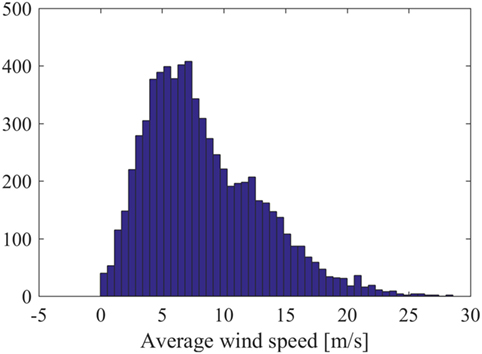
Figure 1. Histogram displaying the distribution of the average wind speeds available for the identification of the model.

FIGURE 2

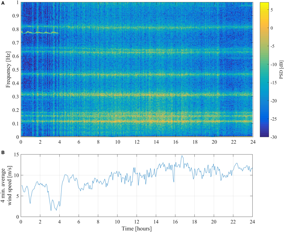
Figure 2. Typical 1-day variation of the PSD of the acceleration response and the average wind speed: (A) PSD (spectrogram)–Hamming window, length 8,192 samples, overlap 5,792 samples; (B) 2 min average wind speed.

4.1.2. Model Identification

4.1.2.1. Modeling of the Short-term Response

An AutoRegressive (AR) model structure is selected to represent the acceleration response on short, 250 s, intervals. The order of the AR model is selected by evaluating different model structures with orders in the range n_a = [1, …, 100]. A subset of 7 days of data is selected to determine the model order. The prior RSS/SSS and Bayesian Information Criterion (BIC) curves, as well as the frequency stabilization plot, displaying the natural frequencies and damping ratios associated with the estimated AR models for increasing orders, are shown in Figure 3. It may be observed that the RSS/SSS tends to favor large AR orders, while the BIC clearly demonstrates several minima, and a global minimum found for the value n_a = 72. The frequency stabilization plot seems to confirm these findings, by demonstrating that the main frequency peaks found in the PSD are accommodated by AR models with order around n_a = 72. Thus, according to the frequency stabilization plot and the BIC curve, the selected model order for subsequent analysis is n_a = 72.

FIGURE 3

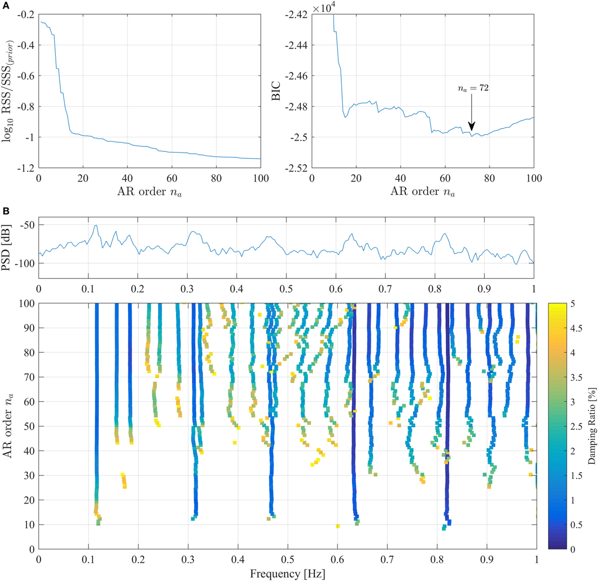
Figure 3. Selection of the order of the AR model. (A) Prior RSS/SSS and BIC curves for increasing model orders n_a = 1, 2, …, 100; (B) frequency stabilization plot of the AR model for increasing model orders with the Welch PSD estimate–Hamming window, length 512 samples, 256 samples overlap.

4.1.2.2. Modeling of the Long-term Response

The long-term acceleration response of the bridge is represented by means of a GP-AR model where the 250 s average wind speed is used as EOP, this is to say ξ. For this purpose, the average wind speed is normalized from the range [0, 30] m/s to the range [0,1] by making ξ = AWS/30, where AWS stands for the 250 s Average Wind Speed. The functional basis used for the expansion of the parameter vector of the model corresponds to the class of Hermite orthogonal polynomials, which satisfy the recurrence relation:

$g_{j+1}\left(\mathit{\xi }\right)=H_j\left(\mathit{\xi }\right)=\mathit{\xi }\cdot H_{j-1}\left(\mathit{\xi }\right)-\left(j-1\right)\cdot H_{j-2}\left(\mathit{\xi }\right),\forall j\ge 2$ (37)

$g_1\left(\mathit{\xi }\right)=H_o\left(\mathit{\xi }\right)=1,g_2\left(\mathit{\xi }\right)=H_1\left(\mathit{\xi }\right)=\mathit{\xi }$

Thus, GP-AR(72) models are estimated using the EM algorithm for increasing basis orders in the range of p = 1, …, 6. For the application of the EM algorithm and validation of the performance of the obtained models, the whole dataset consisting of 7,000 segments of 250 s is separated into training and validation subsets. The training subset is composed by the initial 3,000 segments, while the validation subset is composed by the remaining 4,000 segments. It should be noted that the GP-AR(72) model with p = 1 would correspond to the case when the EOP variable is ignored and the parameter vector is assumed to be Gaussian with constant mean and covariance matrix. The settings used for the application of the EM algorithm are shown in Table 1. Note that the threshold Δ_RSS/SSS is presently utilized instead of Δ_ℒ, as suggested in equation (34), since the RSS/SSS is used to evaluate the convergence of the optimization procedure. Figure 4 shows the RSS/SSS based on prior and posterior residuals, as well as for the training and validation subsets obtained with the GP-AR(72) model with basis orders p = 1, …, 6. The obtained results demonstrate that a GP-AR(72) model with basis order p = 4 provides the best fit in all cases. Furthermore, the validation error results slightly elevated when compared against the training error, thus demonstrating the generalization capability of the model.

FIGURE 4

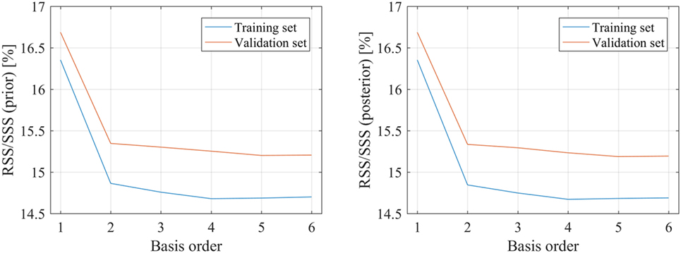
Figure 4. Selection of the basis order of the GP-AR(72) model. Left: prior RSS/SSS obtained for the training and validation subsets; Right: posterior RSS/SSS obtained for the training and validation subsets.

TABLE 1

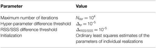
Table 1. Settings of the EM algorithm.

The prior and posterior estimates of the parameter vector as a function of the AWS are shown in Figure 5. The dependency of the parameter estimates on the AWS is evident and is consistent on both the prior and posterior parameter estimates. Nonetheless, in some cases the posterior estimates tend to deviate from the prior at higher AWS values, especially for higher wind speeds. This effect may be due to the reduced amount of signal segments available for higher wind speeds in the construction of the model, as evident in the histogram of wind speeds shown in Figure 1.

FIGURE 5

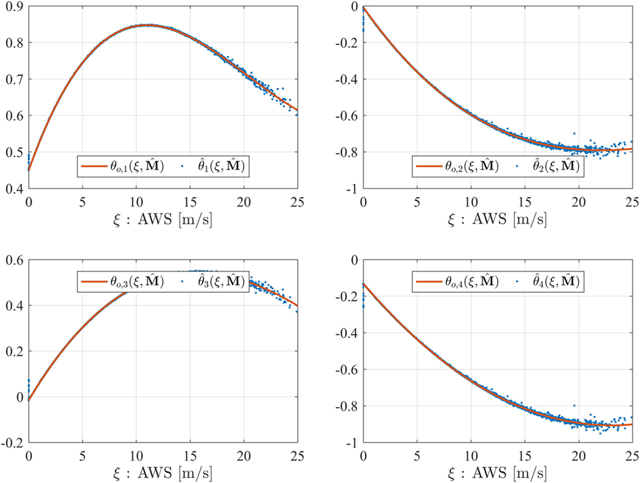
Figure 5. Prior and posterior estimates of the first four parameters of the GP-AR(72)_p=4 model for the average wind speed range from 0 to 25 m/s.

4.1.3. Model-Based Analysis

Once the GP-AR(72)_{p= 4} model has been identified, it is possible to analyze the dynamic characteristics of the acceleration response of the bridge as a function of the average wind speed. In particular, the Power Spectral Density, the natural frequencies and damping ratios are extracted from the identified GP-AR(72)_{p = 4} model. Each one of these quantities are evaluated as follows:

$\text{Characteristic polynomial}:A\left(z,\mathit{\xi }\right)=1+{\displaystyle \sum _{i=1}^{n_a}}{â}_i\left(\mathit{\xi }\right)\cdot z^{-i}$ (38a)

$\text{PSD}:P_{\mathit{yy}}\left(f,\mathit{\xi }\right)=\frac{{\mathrm{\sigma }}_w^2}{{\left|A\left({\text{e}}^{j\mathrm{2\pi }f},\mathit{\xi }\right)\right|}^2}$ (38b)

$\text{Poles}:\left\{{\mathrm{\lambda }}_i\left(\mathit{\xi }\right)\in \mathbb{C},i=1,\dots ,n_a:A\left(\mathrm{\lambda },\mathit{\xi }\right)=0\right\}$ (38c)

$\text{Natural frequencies}:f_{n,i}\left(\mathit{\xi }\right)=\frac{f_s}{\mathrm{2\pi }}\cdot \mathrm{|}\text{ln }{\mathrm{\lambda }}_i\left(\mathit{\xi }\right)\mathrm{|}$ (38d)

$\text{Damping ratios}:{\mathrm{\zeta }}_i\left(\mathit{\xi }\right)=-\text{cos}\left(\text{arg}\left(\text{ln }{\mathrm{\lambda }}_i\left(\mathit{\xi }\right)\right)\right)$ (38e)

Figure 6 shows the GP-AR(72)_{p = 4} model-based PSD, natural frequencies and damping ratios obtained for the range of average wind speeds from 0 to 25 m/s, while frequencies and damping ratios are limited to the ranges [0,500] mHz and [0,10]%, respectively. The model-based PSD and modal quantities demonstrate that both the amplitude and frequency of the vibration are directly influenced by the average wind speed.

FIGURE 6

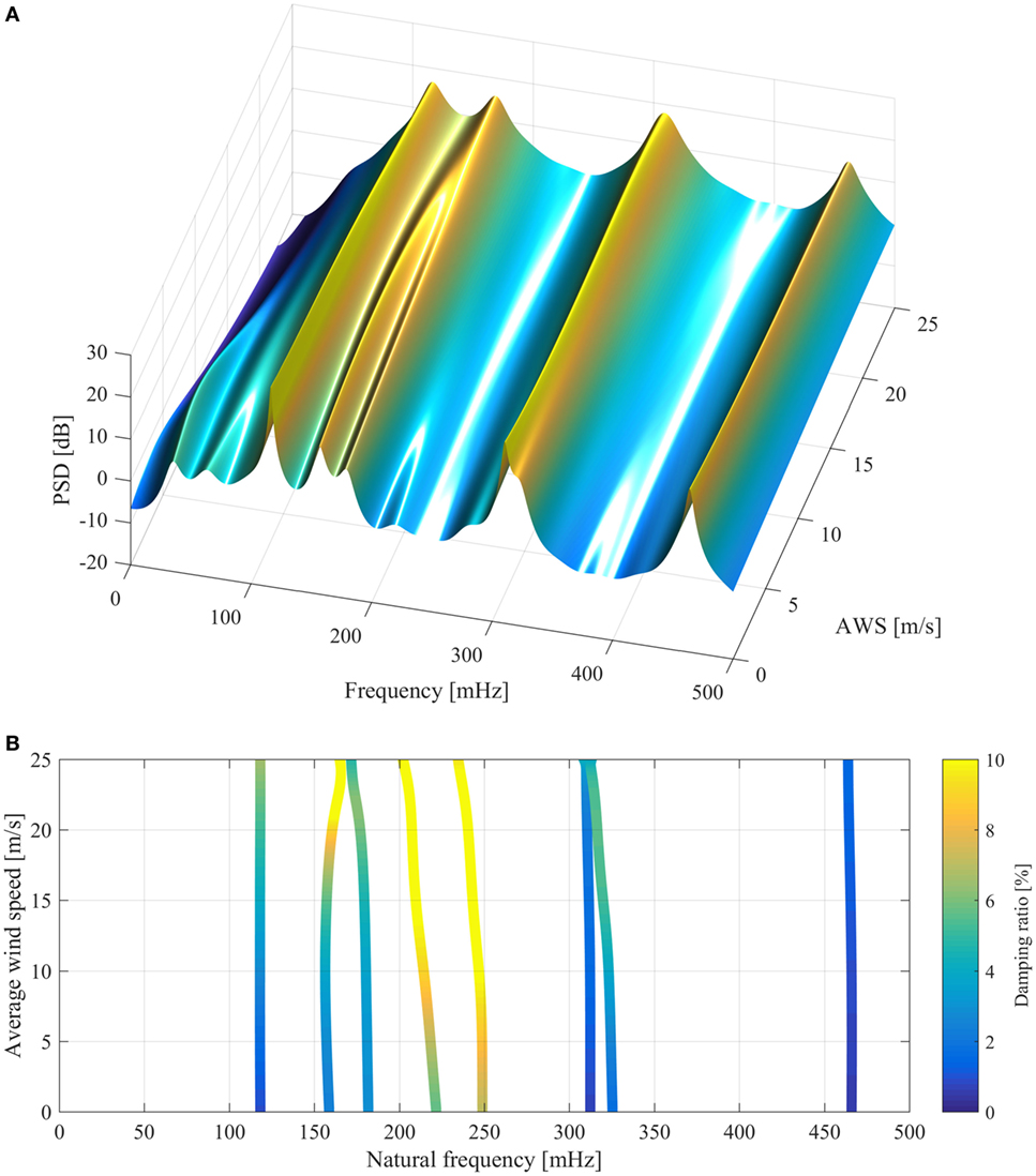
Figure 6. GP-AR(72)_p=4 model-based PSD, natural frequencies, and damping ratios as a function of the average wind speed in the range 0–25 m/s. Frequency range and damping ratio limited to [0, 500] mHz and [0, 10]%, respectively. (A) PSD of the bridge vibration as a function of AWS; (B) natural frequencies and damping ratios as a function of AWS.

A more detailed analysis of the first six natural frequencies and damping ratios obtained from prior and posterior parameter estimates is presented in Figure 7. The posterior estimates are calculated for the complete set of vibration segments based on the estimated GP-AR model. The dispersion of the modal quantities tends to blow up for increasing wind speeds, which in part may be due to the effect of wind and turbulence on the structure. In addition, the difference between prior and posterior estimates of the modal quantities tends to increase when the wind speed is larger than 20 m/s. This effect may be due to the lesser amount of samples acquired from higher wind speeds, which may be leading to increased uncertainty in the parameter estimates. The modal analysis results obtained with the GP-AR model may be contrasted with those previously reported on (Diana et al., 1992; Brownjohn et al., 1994, 2010). In particular, it appears that the modes displayed in Figure 7 correspond to the first, second, third, and eight vertical modes (f_n,1, f_n,2,f_n,3, and f_n,5 respectively), and the first torsional mode of the bridge (f_n,4). Nonetheless, the predicted variation in the first torsional mode appears to be different to that one found with the GP-AR model.

FIGURE 7

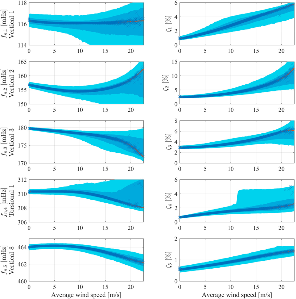
Figure 7. Distribution of selected natural frequencies and damping ratios obtained from the GP-AR(72)_p=4 model. Solid line, modal quantities from prior parameter estimates; dots, modal quantities from posterior parameter estimates; shaded areas, 50 and 90% confidence intervals derived from the parameter mean and covariance matrix. Left column: natural frequencies in mHz; right column: damping ratios.

Confirmation of the modal analysis results shall be sought in a future work, where a vector AR model would be used to represent the two vertical and the horizontal vibration response of the bridge. However, the relatively simpler model utilized in this analysis can be used to track and assess the variability in the modes of the bridge when the wind is blowing from the main direction.

4.2. Simulated Vibration of Operating Wind Turbine Blades

4.2.1. Data Description and Preprocessing

This application focuses on the identification and analysis of the vibration acceleration signals obtained via simulations of a fully operational wind turbine. For a PCE-based treatment on actual tower measurements obtained from an operated wind turbine, the interested reader is referred to Bogoevska et al. (2017). The analyzed wind turbine is the NREL 5 MW reference offshore wind turbine, fully described in Jonkman et al. (2009). The simulation is performed by means of the FAST wind turbine aeroelastic code, which uses a turbulent wind excitation simulated with TurbSim (Jonkman and Buhl, 2005). Acceleration signals are measured at different locations along the span of on one of the blades of the wind turbine on the flap wise direction, as depicted in Figure 8. From these, the acceleration signals measured on the tip of the blade (node 6) are used for further analysis.

FIGURE 8

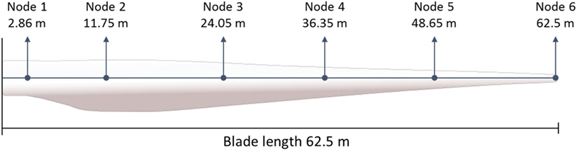
Figure 8. Location of the sensors in the blade of the wind turbine. Acceleration signals are measured on the flapwise direction of the blade (normal to the surface of the page).

Simulations of both turbulent wind and vibration response are computed for a period of 10 min (600 s) with a sampling rate of 200 Hz. Moreover, the instantaneous rotor azimuth is also extracted, which shall be used as the scheduling variable in the model for representation of the short-term response. The obtained acceleration signals are subsequently downsampled at 12.5 Hz for further analysis and processing. An antialiasing low-pass filter is applied before down-sampling. The filter consists of a 100 order FIR filter with cutoff frequency of 5 Hz. The cutoff frequency has been selected in order to preserve the structural modes which are under 4 Hz, and is applied in a forward–backward fashion to compensate the phase delay by using the MATLAB command filtfilt.

A set of 100 simulations is obtained under different 10 min average wind speeds in the range from 5 to 26 m/s. For that purpose, the Latin hypercube sampling algorithm is used to create a set of 100 random average wind speeds within the specified range. Then, a turbulent wind speed time-series is simulated for each 10 min average wind speed, which is subsequently used as input to the FAST simulation software.

It is noted that the present simulated data bears important differences with those published in the previous work (Avendaño-Valencia and Fassois, 2017a), which are summarized as follows: (i) The turbulent wind excitation is simulated over an 8 × 8 grid, in comparison with the 2 × 2 grid used in the previous work. Therefore, the excitation is richer while the vibration response may be more complex. (ii) The sampling rate used for simulation is extended from 25 to 200 Hz so as to improve the convergence of the numerical integration algorithm. (iii) The analysis is performed in a sensor in the blade tip instead of the blade root. A consequence of the previous selections is that the structure of the obtained models may differ significantly with that reported (Avendaño-Valencia and Fassois, 2017a).

4.2.2. Model Identification

4.2.2.1. Modeling of the Short-term Response

The blade vibration signal is represented via a Linear Parameter Varying AR (LPV-AR) model, which uses the instantaneous rotor azimuth as scheduling variable (Avendaño-Valencia and Fassois, 2017a). The selection structure of the LPV-AR model follows the procedure described in Avendaño-Valencia and Fassois (2017a), while the selection of the LPV-AR model structure is guided by the BIC. The obtained BIC curves are shown in Figure 9, from which the model order n_a = 17 and basis order p_a = 5 are selected.

FIGURE 9

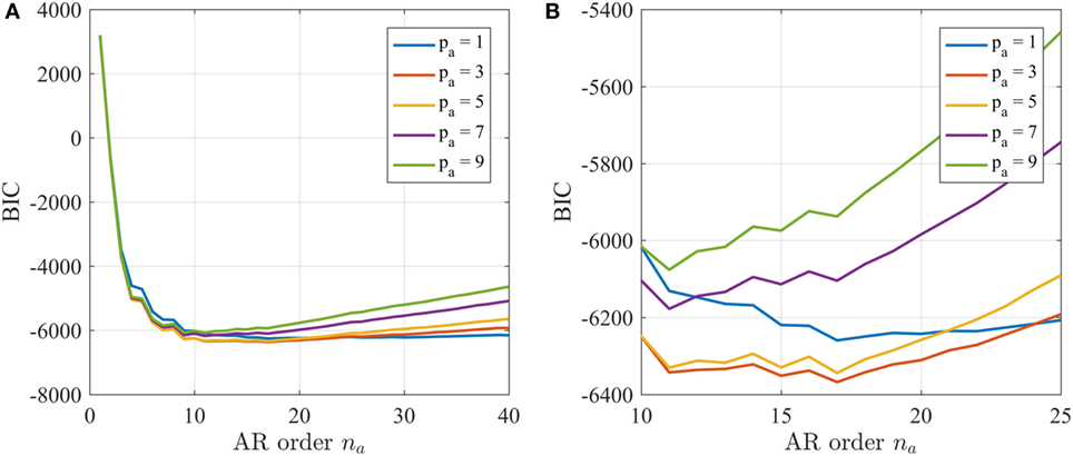
Figure 9. Selection of the LPV-AR model structure: BIC curves for increasing model orders n_a = 1, 2, …, 40 and for different basis orders p_a = 1, 3, …, 9: (A) whole range; (B) detail in the range n_a = [10, 25].

4.2.2.2. Modeling of the Long-term Response

A GP-LPV-AR model is constructed for the representation of the long term response of the blade. For this purpose, the EOP variable ξ is defined as the 10 minute average wind speed (lying in the range [0,30] m/s) normalized within the range [0,1]. The parameter vector of the model is expanded on the Hermite polynomials defined in equation (37).

GP-LPV-AR(17)₅ models with GP basis orders in the range p = 0, 1, …, 6 are estimated using the EM algorithm. The settings of the EM algorithm are similar to those used in the previous example and summarized in Table 1; however, in the present case the thresholds for finalization of the optimization are defined as Δ_p = Δ_RSS/SSS = 10^–6. Figure 10A shows the RSS/SSS based on the prior and posterior prediction errors for increasing orders of the functional basis expansion of the GP. The plot shows totally different behaviors of the prior and posterior errors. In particular, it is evident that the prior prediction error depends on the order of the functional expansion, while the posterior error does not show a significant dependence. This behavior may be expected, since the prior estimates are based solely on the model predictions, while the posterior estimates are adjusted to the observed vibration response. For that same reason, the prior error is a better tool to evaluate the model capabilities. In the present case, according to the prior RSS/SSS curve, a basis order p = 5 is selected.

FIGURE 10

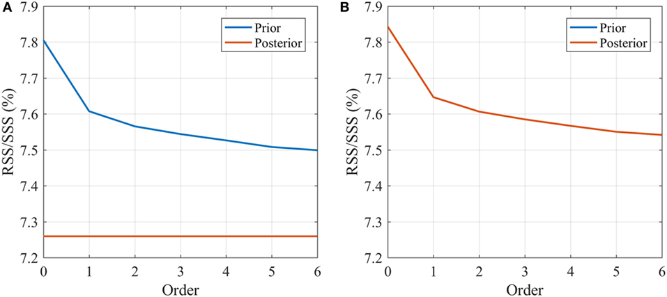
Figure 10. Selection of the order of the GP-LPV-AR models: prior and posterior RSS/SSS curves for increasing GP basis orders p = 0, 1, …, 6, for (A) GP-LPV-AR model; (B) GP-LPV-AR model with principal component regression.

Similarly, a PC-GP-LPV-AR model (based on a Principal Component representation of the regression matrix of the LPV-AR model, as explained in Section 2.4) is used for the long-term identification of the response of the wind turbine. The PC-GP-LPV-AR model is further estimated by means of the EM algorithm, using the same settings applied in the previous GP-LPV-AR model. The Principal Component representation of the regression matrix is carried out using all the components (without dimensionality reduction), however, the covariance matrix of the model parameters is in the present case, diagonal, thus a lower number of hyper-parameters have to be estimated. The obtained prior and posterior RSS/SSS curves obtained with the PC-GP-LPV-AR model are shown in Figure 10B. In this case, the prior and posterior error curves are almost the same, while the overall error is slightly higher than that obtained with the GP-LPV-AR model.

4.2.3. Model-Based Analysis

The dynamics of the wind turbine are analyzed based on the identified GP-LPV-AR(17)_5,5 model. For that purpose, the analysis of the dynamics is based on the “frozen” Power Spectral Density, natural frequencies and damping ratios, which are calculated by means of the following equations:

$\text{“Frozen” characteristic polynomial}:A\left(z,\mathrm{\beta },\mathit{\xi }\right)=1+{\displaystyle \sum _{i=1}^{n_a}}{â}_i\left(\mathrm{\beta },\mathit{\xi }\right)\cdot z^{-i}$ (39a)

$\text{PSD}:P_{\mathit{yy}}\left(f,\mathrm{\beta },\mathit{\xi }\right)=\frac{{\mathrm{\sigma }}_w^2}{{\left|A\left({\text{e}}^{j\mathrm{2\pi }f},\mathrm{\beta },\mathit{\xi }\right)\right|}^2}$ (39b)

$\text{Poles}:\left\{{\mathrm{\lambda }}_i\left(\mathrm{\beta },\mathit{\xi }\right)\in \mathbb{C},i=1,\dots ,n_a:A\left(\mathrm{\lambda },\mathrm{\beta },\mathit{\xi }\right)=0\right\}$ (39c)

$\text{Natural frequencies}:f_{n,i}\left(\mathrm{\beta },\mathit{\xi }\right)=\frac{f_s}{\mathrm{2\pi }}\cdot \mathrm{|}\text{ln}{\mathrm{\lambda }}_i\left(\mathrm{\beta },\mathit{\xi }\right)\mathrm{|}$ (39d)

$\text{Damping ratios}:{\mathrm{\zeta }}_i\left(\mathrm{\beta },\mathit{\xi }\right)=-\text{cos}\left(\text{arg}\left(\text{ln }{\mathrm{\lambda }}_i\left(\mathrm{\beta },\mathit{\xi }\right)\right)\right)$ (39e)

For the present application, these quantities are functions of two variables, namely the instantaneous rotor angle β and the 10 minute average wind speed ξ. In that sense, the “frozen” PSD, natural frequencies and damping ratios are calculated for a single period of rotation of the blades and for the whole range of wind speeds (3–25 m/s). Figure 11 shows the obtained “frozen” PSDs for different wind speeds in the range. The figure indicates that the variability of the characteristics of the dynamic response of the wind turbine both as the rotor azimuth changes, and as the wind speed increases. In particular, it can be observed that for all the wind speeds, an important increment in the power of the vibration response is evident at about two-thirds of a full rotation. This event may be associated with the blade passing in front of the tower. Moreover, it is also evident that as the wind speed increases, the overall power of the vibration response increases as well. The total power difference when the wind speed changes from 5 to 25 m/s is about 20 dB or a whole magnitude level.

FIGURE 11

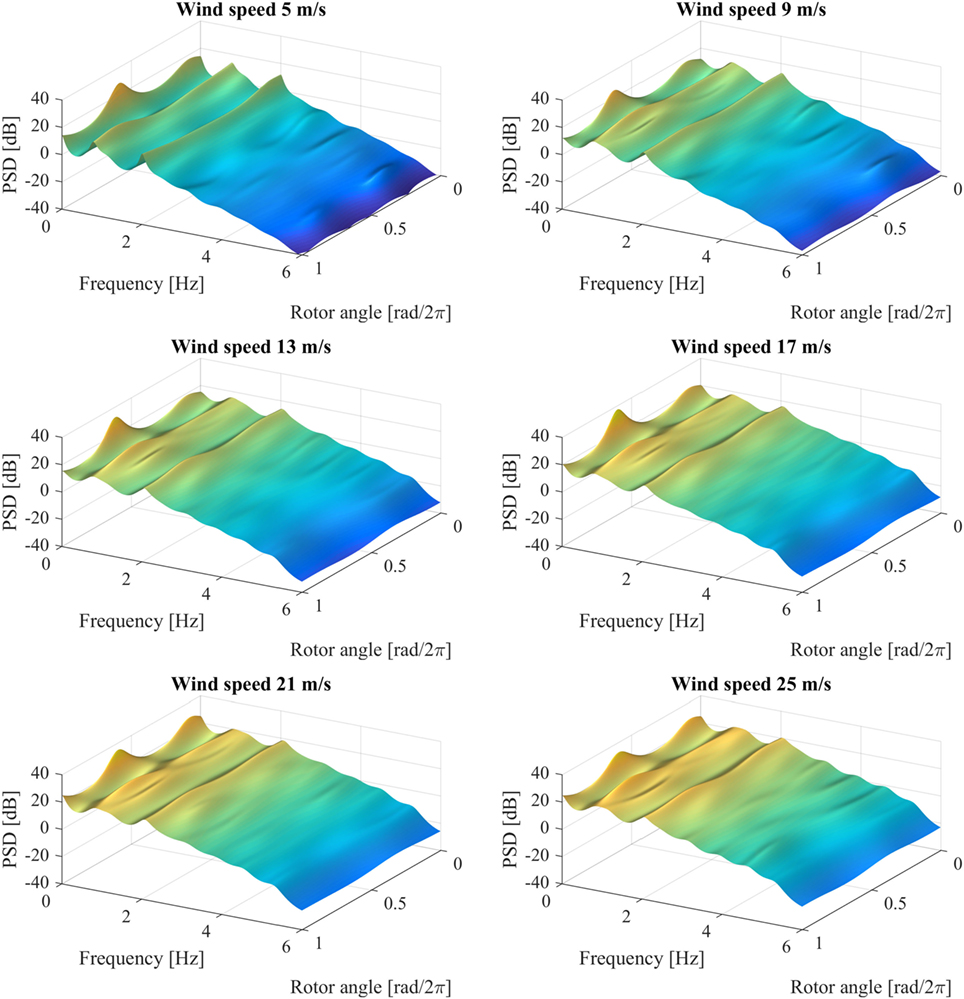
Figure 11. GP-LPV-AR model-based “frozen” Power Spectral Density evaluated for a full rotation period of the wind turbine blade, and for increasing wind speeds.

Average values of the “frozen” natural frequencies and damping ratios and their respective confidence intervals may be drawn from the obtained GP-LPV-AR model. The procedure is similar to that performed in the previous application example. Three modes are selected for this analysis, namely the pair of modes located around 1 Hz, and the mode located around 2 Hz. The selected average “frozen” natural frequencies and damping ratios are shown in Figure 12. In the obtained curves is clear the dependency of both natural frequency and damping ratio on the wind speed. Particularly, for modes 1 and 3 there is an increase on the damping ratio, while for mode 2 the damping ratio tends to decrease as the wind speed does. In addition, the natural frequencies tend to increase with the wind speed as well. The confidence intervals are in general well bounded, and in particular it is clear that the estimates of the damping ratios are reliable.

FIGURE 12

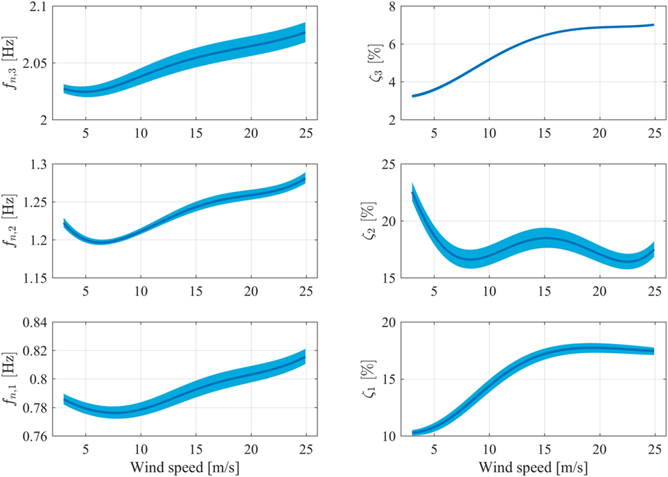
Figure 12. GP-LPV-AR model-based average “frozen” natural frequencies and damping ratios of the wind turbine blade response evaluated for increasing wind speeds. Solid line indicates the average value, while shaded areas indicate estimates of the 95% confidence intervals.

5. Concluding Remarks

This work has been devoted to a Gaussian Process time-series modeling framework for the representation of the long-term dynamics of structures operating under variable environmental and operational conditions. The model definitions plus an identification method based on the Expectation-Maximization algorithm have been presented. In addition, an optional parameter reduction technique based on Principal Component Regression has been introduced as a method to reduce the number of parameters to be estimated in the representation. The resulting GP time-series methods provide an appealing alternative for the representation of the complex dynamics of vibrating structures operating under variable environmental and operational conditions.

A potential limitation of the GP time-series modeling methodology, as presented in this work, is that the innovations variance of the time-series model is assumed to be constant. The adoption of a constant innovations variance may hinder the representation of changing power in the vibrational response of the structure according to environmental and operational conditions. A solution for this limitation is to define a GP to represent the dependence of the innovations variance on the EOPs, in the same manner as already explained for the coefficients of the time-series model. Toward this end, it would be further necessary to modify the EM algorithm for the estimation of the parameters of the innovations variance GP.

The proposed GP time-series modeling method offers a promising tool for assimilation in damage diagnosis algorithms. For this purpose, a key element lies in formalizing the selection of the conditions used for training of the model, namely, specification of the range of environmental and operational conditions under which the GP time-series model is able to lead to a robust decision. An exploratory study on this issue can be found in Avendaño-Valencia and Chatzi (2017), and will be extended as future work.

Author Contributions

LA-V has developed the mathematical techniques involved in this work and performed the simulations shown in the case studies. He has further carried out the major part of the writing and organization of the text. EC has collaborated on the method’s development, writing, and proof-reading of the document and has cross-checked the mathematical techniques. JB has provided the vibration data of the Humber bridge and has further contributed to the scientific writing. KK contributed to the revised version of the work by providing the complete bridge vibration data used in the application example on the Humber bridge. In addition, he participated in the revision of the manuscript pre-prints and in the approval of the finalized version.

Conflict of Interest Statement

The authors declare that the research was conducted in the absence of any commercial or financial relationships that could be construed as a potential conflict of interest.

Funding

The authors gratefully acknowledge the support of the ETH Zurich Postdoctoral Fellowship FEL-45 14-2 “A data-driven computational framework for damage identification and life-cycle management of wind turbine facilities.” In addition, EC would further like to acknowledge the ERC Starting Grant award (ERC-2015-StG 679843) on the topic of “Smart Monitoring, Inspection and Life-Cycle Assessment of Wind Turbines.”

References

Avendaño-Valencia, L., and Chatzi, E. (2017). “Sensitivity driven robust vibration-based damage diagnosis under uncertainty through hierarchical bayes time-series representations,” in Proceedings of X International Conference on Structural Dynamics, EURODYN 2017, Rome, Italy.

Google Scholar

Avendaño-Valencia, L. D., Chatzi, E. N., and Spiridonakos, M. D. (2015a). “Non-stationary random coefficient models for vibration-based shm in structures influenced by strong operational and environmental variability,” in International Workshop on Structural Health Monitoring 2015, Stanford, CA, USA.

Google Scholar

Avendaño-Valencia, L. D., Chatzi, E. N., and Spiridonakos, M. D. (2015b). “Surrogate modeling of nonstationary systems with uncertain properties,” in Proceedings of the European Safety and Reliability Conference ESREL, 2015, Zürich, Switzerland.

Google Scholar

Avendaño-Valencia, L. D., and Fassois, S. D. (2015). “On multiple-model linear-parameter-varying based shm for time-dependent structures under uncertainty,” in International Conference Surveillance 8 (France: Roanne Institute of Technology).

Google Scholar

Avendaño-Valencia, L. D., and Fassois, S. D. (2017a). Damage/fault diagnosis in an operating wind turbine under uncertainty via a vibration response Gaussian mixture random coefficient model based framework. Mech. Syst. Signal Process. 91, 326–353. doi: 10.1016/j.ymssp.2016.11.028

CrossRef Full Text | Google Scholar

Avendaño-Valencia, L. D., and Fassois, S. D. (2017b). Gaussian mixture random coefficient model based framework for SHM in structures with time-dependent dynamics under uncertainty. Mech. Syst. Signal Process. 97, 59–83. doi:10.1016/j.ymssp.2017.04.016

CrossRef Full Text | Google Scholar

Bair, E., Hastie, T., Paul, D., and Tibshirani, R. (2006). Prediction by supervised principal components. J. Am. Stat. Assoc. 101, 119–137. doi:10.1198/016214505000000628

CrossRef Full Text | Google Scholar

Basu, P., Rudoy, D., and Wolfe, P. J. (2009). “A nonparametric test for stationarity based on local Fourier analysis,” in IEEE International Conference on Acoustics, Speech and Signal Processing, Taipei, 3005–3008.

Google Scholar

Bogoevska, S., Spiridonakos, M., Chatzi, E. N., Dumova-Jovanoska, E., and Höffer, R. (2017). A data-driven diagnostic framework for wind turbine structures: a holistic approach. Sensors 17, 1–28. doi:10.3390/s17040720

PubMed Abstract | CrossRef Full Text | Google Scholar

Borgnat, P., Flandrin, P., Honeine, P., Richard, C., and Xiao, J. (2010). Testing stationarity with surrogates: a time-frequency approach. IEEE Trans. Signal Process. 58, 3459–3470. doi:10.1109/TSP.2010.2043971

CrossRef Full Text | Google Scholar

Brownjohn, J., Boccionlone, M., Curami, A., Falco, M., and Zasso, A. (1994). Humber bridge full-scale measurement campaigns 1990-1991. J Wind Eng. Ind. Aerodyn. 52, 185–218. doi:10.1016/0167-6105(94)90047-7

CrossRef Full Text | Google Scholar

Brownjohn, J., Magalhaes, F., Caetano, E., and Cunha, A. (2010). Ambient vibration re-testing and operational modal analysis of the Humber Bridge. Eng. Struct. 32, 2003–2018. doi:10.1016/j.engstruct.2010.02.034

CrossRef Full Text | Google Scholar

Deraemaeker, A., Reynders, E., Roeck, G. D., and Kullaa, J. (2008). Vibration-based structural health monitoring using output-only measurements under changing environment. Mech. Syst. Signal Process. 22, 34–56. doi:10.1016/j.ymssp.2007.07.004

CrossRef Full Text | Google Scholar

Diana, G., Cheli, F., Zasso, A., Collina, A., and Brownjohn, J. (1992). Suspension bridge parameter identification in full scale test. J. Wind Eng. Ind. Aerodyn. 41-44, 165–176. doi:10.1016/0167-6105(92)90404-X

CrossRef Full Text | Google Scholar

Hastie, T., Tibshirani, R., and Friedman, J. (2009). The Elements of Statistical Learning, Data Mining, Inference, and Prediction. Springer Series in Statistics. New York: Springer.

Google Scholar

Jonkman, J. M., and Buhl, M. L. (2005). FAST User’s Guide. Technical Report. Battelle, CO: National Renewable Energy Laboratory, U.S. Department of Energy, Office of Energy Efficiency and Renewable Energy.

Google Scholar

Jonkman, J. M., Butterfield, S., Musial, W., and Scott, G. (2009). Definition of a 5-MW Reference Wind Turbine for Offshore System Development. Technical Report. Battelle, CO: National Renewable Energy Laboratory, U.S. Department of Energy, Office of Energy Efficiency and Renewable Energy.

Google Scholar

Kay, S. (2008). A new nonstationarity detector. IEEE Trans. Signal Process. 56, 1440–1451. doi:10.1109/TSP.2007.909346

CrossRef Full Text | Google Scholar

Kopsaftopoulos, F., Nardari, R., Li, Y.-H., and Chang, F.-K. (2018). A stochastic global identification framework for aerospace structures operating under varying flight states. Mech. Syst. Signal Process. 98, 425–447. doi:10.1016/j.ymssp.2017.05.001

CrossRef Full Text | Google Scholar

Ljung, L. (1999). System Identification: Theory for the User, 2nd Edn. Prentice Hall PTR.

Google Scholar

Poulimenos, A., and Fassois, S. D. (2006). Parametric time-domain methods for non-stationary random vibration modeling and analysis: a critical survey and comparison. Mech. Syst. Signal Process. 20, 763–816. doi:10.1016/j.ymssp.2005.10.003

CrossRef Full Text | Google Scholar

Rahbari, R., Niu, J., Brownjohn, J., and Koo, K.-Y. (2015). Structural identification of Humber Bridge for performance prognosis. Smart Struct. Syst. 15, 665–682. doi:10.12989/sss.2015.15.3.665

CrossRef Full Text | Google Scholar

Rasmussen, C., and Williams, C. (2006). Gaussian Processes for Machine Learning. MIT Press.

Google Scholar

Sakellariou, J. S., and Fassois, S. D. (2016). Functionally pooled models for the global identification of stochastic systems under different pseudo-static operating conditions. Mech. Syst. Signal Process. 72-73, 785–807. doi:10.1016/j.ymssp.2015.10.018

CrossRef Full Text | Google Scholar

Shumway, R. H., and Stoffer, D. S. (2011). Time Series Analysis and Its Applications. New York: Springer.

Google Scholar

Sohn, H. (2007). Effects of environmental and operational variability on structural health monitoring. Philos. Trans. A Math. Phys. Eng. Sci. 365, 539–560. doi:10.1098/rsta.2006.1935

PubMed Abstract | CrossRef Full Text | Google Scholar

Spiridonakos, M. D., and Chatzi, E. N. (2014). “Polynomial chaos expansion models for SHM under environmental variability,” in Proceedings of the 9th International Conference on Structural Dynamics (EURODYN 2014), Porto, Portugal, 2393–2398.

Google Scholar

Spiridonakos, M. D., and Chatzi, E. N. (2015). Metamodeling of dynamic nonlinear structural systems through polynomial chaos NARX models. Comput. Struct. 157, 99–113. doi:10.1016/j.compstruc.2015.05.002

CrossRef Full Text | Google Scholar

Spiridonakos, M. D., Chatzi, E. N., and Sudret, B. (2016). Polynomial Chaos expansion models for the monitoring of structures under operational variability. ASCE-ASME J. Risk Uncertain. Eng. Syst. A Civ. Eng. 2, B4016003. doi:10.1061/AJRUA6.0000872

CrossRef Full Text | Google Scholar

Vapnik, V. N. (2000). The Nature of Statistical Learning Theory. New York: Springer.

Google Scholar

Worden, K., Sohn, H., and Farrar, C. (2002). Novelty detection in a changing environment: regression and interpolation approaches. J. Sound Vibr. 258, 741–761. doi:10.1006/jsvi.2002.5148

CrossRef Full Text | Google Scholar

Yan, A.-M., Kerschen, G., Boe, P. D., and Golinval, J.-C. (2005). Structural damage diagnosis under varying environmental conditions. Part I: a linear analysis. Mech. Syst. Signal Process. 19, 847–864. doi:10.1016/j.ymssp.2004.12.003

CrossRef Full Text | Google Scholar

Appendix

A. Demonstrations

A.1. Demonstration of the PDF in Equation (10)

This section aims to demonstrate the PDF of the dynamic response vector $\mathit{y}={\left[\begin{array}{ccc}\hfill y\left[1\right]\hfill & \hfill \cdots \hfill & \hfill y\left[N\right]\hfill \end{array}\right]}^T$ given the parameter vector θ and the regression matrix $\mathbf{\Phi }={\left[\begin{array}{ccc}\hfill \mathit{\varphi }\left(\mathit{z}\left[1\right]\right)\hfill & \hfill \cdots \hfill & \hfill \mathit{\varphi }\left(\mathit{z}\left[N\right]\right)\hfill \end{array}\right]}^T$. For that purpose, consider the PDF:

$p\left(\mathit{y}|\mathit{\theta },\mathbf{\Phi }\right)={\displaystyle \prod _{t=1}^N}p\left(y\left[t\right]|\mathit{\theta },\mathit{\varphi }\left(\mathit{z}\left[t\right]\right)\right)$ (A1)

substituting equation (8) and displaying the Gaussian distribution as an exponential function, yields:

$p\left(\mathit{y}|\mathit{\theta },\mathbf{\Phi }\right)={\displaystyle \prod _{t=1}^N}{\mathcal{N}}_{y\left[t\right]}\left(y\left[t|t-1\right],{\mathrm{\sigma }}_w^2\right)={\displaystyle \prod _{t=1}^N}{\left(\mathrm{2\pi }{\mathrm{\sigma }}_w^2\right)}^{-1/2}\cdot \exp \left(-\frac{1}{2{\mathrm{\sigma }}_w^2}{\left(y\left[t\right]-{\mathit{\varphi }}^T\left(\mathit{z}\left[t\right]\right)\cdot \mathit{\theta }\right)}^2\right)$ (A2)

applying the product operator, yields:

$\begin{array}{l}p\left(\mathit{y}|\mathit{\theta },\mathbf{\Phi }\right)={\left(\mathrm{2\pi }{\mathrm{\sigma }}_w^2\right)}^{-N/2}\cdot \text{exp}\left(-\frac{1}{2{\mathrm{\sigma }}_w^2}{\displaystyle \sum _{t=1}^N}\left(y\left[t\right]-{\mathit{\varphi }}^T\left(\mathit{z}\left[t\right]\right)\cdot \mathit{\theta }\right)\right)\hfill \\ ={\left(\mathrm{2\pi }\right)}^{-N/2}\cdot \mathrm{|}{\mathrm{\sigma }}_w^2\cdot {\mathit{I}}_N{\mathrm{|}}^{-1/2}\cdot \exp \left(-\frac{1}{2{\mathrm{\sigma }}_w^2}{\displaystyle \sum _{t=1}^N}{\left(y\left[t\right]-{\mathit{\varphi }}^T\left(\mathit{z}\left[t\right]\right)\cdot \mathit{\theta }\right)}^2\right)\hfill \end{array}$ (A3)

Then, operating in the sum inside of the exponential function, leads to:

$\begin{array}{l}{\displaystyle \sum _{t=1}^N}{\left(y\left[t\right]-{\mathit{\varphi }}^T\left(\mathit{z}\left[t\right]\right)\cdot \mathit{\theta }\right)}^2={\displaystyle \sum _{t=1}^N}\left(y\left[t\right]-{\mathit{\varphi }}^T\left(\mathit{z}\left[t\right]\right)\cdot \mathit{\theta }\right)\cdot \left(y\left[t\right]-{\mathit{\varphi }}^T\left(\mathit{z}\left[t\right]\right)\cdot \mathit{\theta }\right)\hfill \\ ={\left[\begin{array}{c}\hfill y\left[1\right]-{\mathit{\varphi }}^T\left(\mathit{z}\left[1\right]\right)\cdot \mathit{\theta }\hfill \\ \hfill y\left[2\right]-{\mathit{\varphi }}^T\left(\mathit{z}\left[2\right]\right)\cdot \mathit{\theta }\hfill \\ \hfill ⋮\hfill \\ \hfill y\left[N\right]-{\mathit{\varphi }}^T\left(\mathit{z}\left[N\right]\right)\cdot \mathit{\theta }\hfill \end{array}\right]}^T\cdot \left[\begin{array}{c}\hfill y\left[1\right]-{\mathit{\varphi }}^T\left(\mathit{z}\left[1\right]\right)\cdot \mathit{\theta }\hfill \\ \hfill y\left[2\right]-{\mathit{\varphi }}^T\left(\mathit{z}\left[2\right]\right)\cdot \mathit{\theta }\hfill \\ \hfill ⋮\hfill \\ \hfill y\left[N\right]-{\mathit{\varphi }}^T\left(\mathit{z}\left[N\right]\right)\cdot \mathit{\theta }\hfill \end{array}\right]\hfill \\ ={\left(\left[\begin{array}{c}\hfill y\left[1\right]\hfill \\ \hfill y\left[2\right]\hfill \\ \hfill ⋮\hfill \\ \hfill y\left[N\right]\hfill \end{array}\right]-\left[\begin{array}{c}\hfill {\mathit{\varphi }}^T\left(\mathit{z}\left[1\right]\right)\hfill \\ \hfill {\mathit{\varphi }}^T\left(\mathit{z}\left[2\right]\right)\hfill \\ \hfill ⋮\hfill \\ \hfill {\mathit{\varphi }}^T\left(\mathit{z}\left[N\right]\right)\hfill \end{array}\right]\cdot \mathit{\theta }\right)}^T\cdot \left(\left[\begin{array}{c}\hfill y\left[1\right]\hfill \\ \hfill y\left[2\right]\hfill \\ \hfill ⋮\hfill \\ \hfill y\left[N\right]\hfill \end{array}\right]-\left[\begin{array}{c}\hfill {\mathit{\varphi }}^T\left(\mathit{z}\left[1\right]\right)\hfill \\ \hfill {\mathit{\varphi }}^T\left(\mathit{z}\left[2\right]\right)\hfill \\ \hfill ⋮\hfill \\ \hfill {\mathit{\varphi }}^T\left(\mathit{z}\left[N\right]\right)\hfill \end{array}\right]\cdot \mathit{\theta }\right)\hfill \end{array}$ (A4)

and thus:

${\displaystyle \sum _{t=1}^N}{\left(\mathit{y}\left[t\right]-{\mathit{\varphi }}^T\left(\mathit{z}\left[t\right]\right)\cdot \mathit{\theta }\right)}^2={\left(\mathit{y}-{\mathit{\varphi }}^T\cdot \mathit{\theta }\right)}^T\cdot \left(\mathit{y}-{\mathbf{\Phi }}^T\cdot \mathit{\theta }\right)$ (A5)

Then, after putting everything together, the following result is obtained:

$\begin{array}{l}p\left(\mathit{y}\mathrm{|}\mathit{\theta },\mathbf{\Phi }\right)={\left(\mathrm{2\pi }\right)}^{-N/2}\cdot \mathrm{|}{\mathrm{\sigma }}_w^2\cdot {\mathit{I}}_N{\mathrm{|}}^{-1/2}\cdot \exp \left(-\frac{1}{2{\mathrm{\sigma }}_w^2}{\left(\mathit{y}-{\mathbf{\Phi }}^T\cdot \mathit{\theta }\right)}^T\cdot \left(\mathit{y}-{\mathbf{\Phi }}^T\cdot \mathit{\theta }\right)\right)\hfill \\ ={\mathcal{N}}_y\left({\mathbf{\Phi }}^T\cdot \mathit{\theta },{\mathrm{\sigma }}_w^2\cdot {\mathit{I}}_N\right)\hfill \end{array}$ (A6)