- 1Department of Civil, Environmental and Architectural Engineering, University of Colorado Boulder, Boulder, CO, United States
- 2United States Geological Survey, Golden, CO, United States
- 3Department of Civil and Environmental Engineering, University of Western Ontario, London, ON, Canada
Earthquake ground motions induced by a scenario event are spatially (partially) correlated and (partially) coherent. Simulated ground motion records can be used to carry out nonlinear inelastic time history analysis for a portfolio of buildings to estimate the seismic loss, which is advantageous as there is no need to develop and apply empirical ground motion prediction equations and the ductility demand rules, or to search the scenario-compatible recorded records at selected sites that may not exist. Further, if the structures being considered are sensitive to the orientation of the excitation, multiple-component ground motion records are needed. For the simulation of such ground motion records, previous studies have shown that correlation and coherency between any pair of ground motion components need to be incorporated. In this study, the seismic loss of a portfolio of hypothetical buildings in downtown Vancouver under bidirectional horizontal ground motions due to a scenario Cascadia event is estimated by using simulated bidirectional ground motion records that include realistic correlation and coherency characteristics. The hysteretic behaviors of the buildings are described by bidirectional Bouc–Wen model. The results show that the use of unidirectional ground motions and single-degree-of-freedom system structural model may underestimate the aggregated seismic loss.
Introduction
Seismic loss estimation for a portfolio of buildings under scenario events generally requires three sets of information. The first one is the scenario event and its associated multiple component ground motions at the spatially distributed sites of the buildings. The second set is associated with non-linear inelastic dynamic characteristics of the buildings and their responses or degree of damage under seismic excitations. The third set contains the damage loss functions for different structure types and degree of damage. For simplicity, seismic loss estimation for a portfolio of buildings is often carried out by using the ground motion measures such as the peak ground acceleration (PGA) and spectral acceleration (SA) for random orientation. The structural responses and damage are then represented using predetermined fragility curves based on experience, expert opinion, or numerical analysis and experimental investigation [HAZUS-Earthquake, Federal Emergency Management Agency (FEMA) and the National Institute of Building Sciences (NIBS), 2003; Whitman et al., 1997]. The seismic risk of a portfolio of buildings is then estimated by incorporating the (uncertainty in the) ground motion measures of the scenario event, the fragility curves, and the damage cost functions. Therefore, significant computing task in this approach, in terms of structural responses, is to establish the fragility curves for generic structures of different structural types. Instead of using fragility curves, Goda and Hong(2008a,b) considered that each building can be approximated as a non-linear inelastic single-degree-of-freedom (SDOF) system, and the spatially distributed buildings are subjected to spatially correlated ground motion measures. To assess the degree of damage, use of the ductility demand rules for bilinear systems developed based on selected ground motions (Hong and Hong, 2007) were considered. It was shown that the consideration of realistic spatial correlation is crucial in assessing the tail of the probability distribution of seismic loss of a portfolio of buildings. The approach avoids the need for predetermining the fragility curve of the degree of damage conditioned on the ground motion measure such as SA, and approximately takes into account dynamic and inelastic characteristics of each of the buildings. However, the ductility demand rules could be affected by records from different earthquake types (Hong et al., 2010).
To avoid the need to develop empirical ductility demand rules for structures having different hysterical behavior and different ground motion characteristics, Liu and Hong (2015a) considered that the structural responses and damage levels can be estimated directly through the time history analysis under spatially correlated and coherent ground motion excitations. Their study, again, showed the importance of considering realistic spatial correlation in assessing the tail of the probability distribution of seismic loss of a portfolio of buildings. The approach of using time history analysis is also advantageous as there is no need to develop and apply empirical ground motion prediction equations. Furthermore, the use of the simulated ground motion records avoids the search for the scenario compatible actual records at the considered building sites that are unlikely to be available in the existing database of ground motion records.
For the simulation of the ground motion records, both the spatial correlation (Goda and Hong, 2008a; Jayaram and Baker, 2009; Liu et al., 2012) and spatial coherency (Abrahamson et al., 1991; Zerva, 2009) need to be taken into account. The coherency between two ground motion record components can be estimated from the power spectral density functions of the records; it represents the correlation between the random phase variations. The spatial correlation is used to measure the correlation of ground motion measures such as the PGA or SA at two sites. Furthermore, seismic events cause multidirectional ground motions. Methodology for the simulation of ground motion records that considers both spatial correlation and coherency for multidirectional excitations at multiple sites was presented in Hong and Liu (2014), Liu and Hong(2015a,b) based on stochastic simulations (e.g., point source model and finite-fault model) (Motazedian and Atkinson, 2005; Atkinson et al., 2009). These methods apply partially (and directional-dependent) coherent white noises generated using spectral representation method as the input for stochastic simulation techniques and incorporates spatially correlated Fourier amplitude spectra (FAS).
It must be emphasized that although multidirectional synthetic ground motion record components at multiple sites can be simulated, the estimation of seismic loss by considering multidirectional excitations for a portfolio of buildings for a scenario event has not been investigated. This can be important as the seismic response of buildings could be sensitive to multidirectional excitations (Clough and Penzien, 2003; Zerva, 2009), and a building could be modeled approximately by using a non-linear inelastic 2-degree-of-freedom (2DOF) system in lieu of a SDOF system, where each degree of freedom is associated with one of the two orthogonal horizontal directions. The hysteretic behavior of the 2DOF system could be modeled by the Bouc–Wen model (Wen, 1976; Lee and Hong, 2010), which can be used to reproduce sophisticated inelastic behavior of structural components/systems under cyclic loadings.
The main objectives of this study are to provide an overall framework to estimate seismic loss of a group of buildings under multidirectional excitations, and to investigate the effect of bidirectional ground motions on the aggregate seismic loss of buildings for a scenario event. The tasks include (a) simulating ground motion record components in two horizontal orthogonal directions at multiple sites for a scenario event such as that from the Cascadia subduction zone considering spatial (and directional) correlation and coherency models derived from historical records; (b) applying the simulated records in estimating seismic responses, and aggregate losses of a portfolio of buildings for the scenario event. In the following, first, the framework to estimate the aggregate seismic loss for a portfolio of buildings under multidirectional ground motions is described. The overall framework is then illustrated by a numerical example focused on the estimation of the seismic loss of a portfolio of buildings located in downtown Vancouver under a scenario Cascadia event, though we expect the conclusions of this study are independent of the study area.
Framework for Estimating Seismic Loss of a Portfolio of Buildings Considering Bidirectional Horizontal Ground Motions
In this section, the proposed framework to estimate the aggregate seismic loss of a group of buildings is presented. The procedure consists of three major components: the simulation of ground motion records (or field); the approximation of structural modeling and nonlinear inelastic analysis, and the estimation and characterization of aggregate seismic loss using the damage cost functions. For the simulation of ground motion records, approach and empirical correlation and coherency models among ground motion components given in the literature (Hong and Liu, 2014; Liu and Hong, 2015b) are considered, except that the reference FAS and time modulation function of the records are defined using the stochastic finite-fault method (Atkinson et al., 2009). For efficiency, the bidirectional Bouc–Wen model is used to calculate the non-linear inelastic response of the 2DOF system and the damage factor; the aggregated seismic loss for the portfolio of buildings is estimated by adopting cost functions in the literature.
Simulation of Bidirectional Ground Motion Records at Multiple Sites
For the simulation of ground motion record components in two horizontal orthogonal directions at multiple sites, it is considered that the reference FAS and the time modulating functions for a random horizontal component can be defined based on the finite-fault model (Motazedian and Atkinson, 2005; Atkinson et al., 2009). As the two horizontal orthogonal ground motion components at a site are considered to be random with respect to the source-to-site orientation, both the reference FAS and the time modulating function for one direction that is perpendicular to the other orientation is considered to be the identical.
To obtain the reference FAS and time modulating function at the j-th site, simulation by using the finite-fault model is carried out nG times for a considered scenario event with moment magnitude M. For each simulated record component, the FAS is evaluated and the time window profile (i.e., time modulating function) is estimated using the Hilbert transform. The reference FAS denoted as yj(M, Rj, f), and the time modulating function are then calculated by averaging over nG simulations, where f is the frequency in Hz and Rj is the distance from the j-th site to finite-fault source (i.e., closest distance to the fault plane). Based on the obtained reference yj(M, Rj, f), and the time modulating function, the simulation of the ground motion record components in two horizontal orthogonal directions are carried out as illustrated in Figure 1 and outlined below (Hong and Liu, 2014):
(a) Generate two band-limited noises with 0 mean and unit variance at each considered site that are compatible with a specified target spatial coherency;
(b) Apply the corresponding time modulating function to the sampled noises at each site;
(c) Calculate and normalize the FAS of each time-modulated time series of the noises by its square-root of the mean squared amplitude spectrum;
(d) Multiply the normalized spectrum by its corresponding reference FAS and by the sampled spatial correlated scaling factor; and,
(e) Apply the inverse Fourier transform to the spectra obtained in step (d) to compute the acceleration ground motion time history.
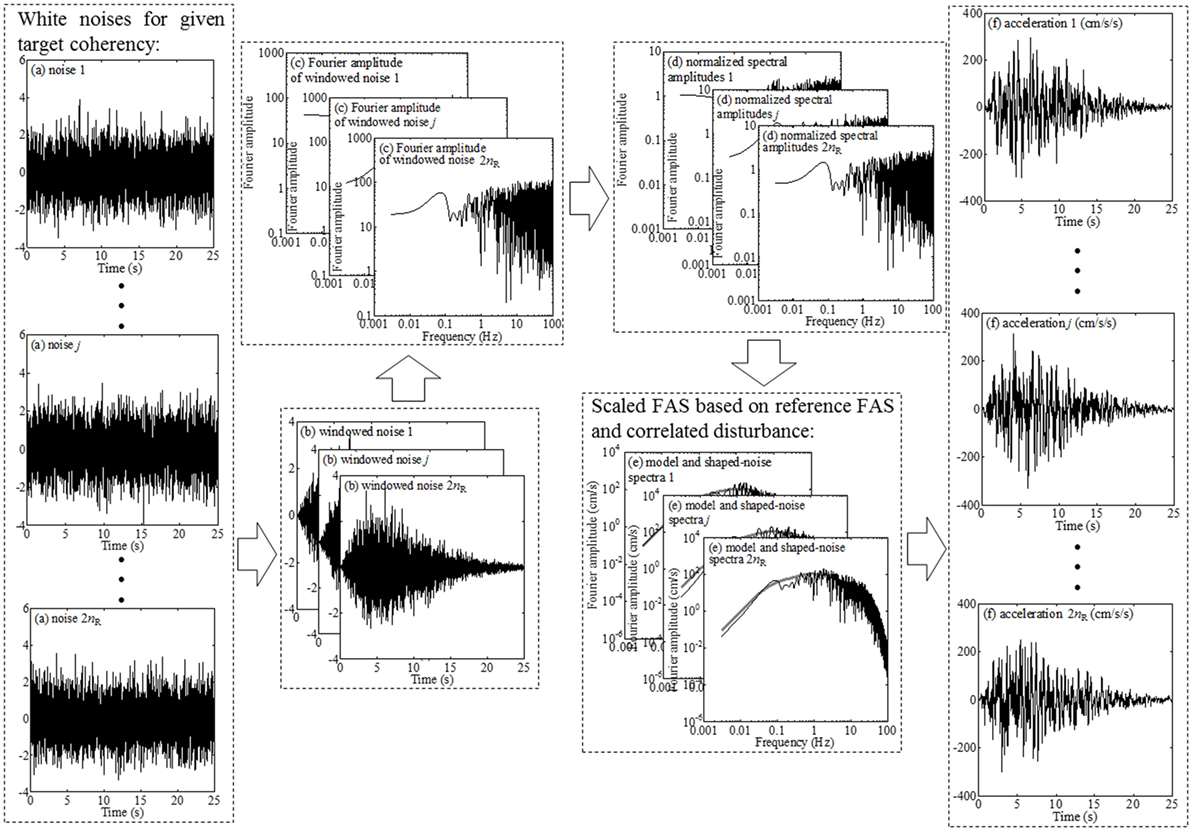
Figure 1. Illustration of simulating spatially correlated and coherent record using the extended finite-fault model.
The target coherency functions needed in Step (a) by considering the j-th and k-th sites is denoted by , where j, k = 1, …, nR represents the sites, p, q = 1 or 2 represents the first and second horizontal ground motion component (for a common coordinate system) and Δ (kilometers) is the distance between the j-th and k-th sites. By taking into account the symmetry and the fact that by definition, there are six remaining coherency functions need to be considered: , , , , , and . The coherency function for two ground motion components along the same orientation (i.e., or ), can be expressed as (Harichandran and VanMarcke, 1986),
where ΔP is the projection of the separation distance Δ in the direction of wave propagation; vap (kilometer per second) represents the apparent velocity; 2πf ΔP/vap represents phase angle of the wave passage effect (Der Kiureghian, 1996); the lagged coherency is given by (Harichandran and VanMarcke, 1986),
in which , and A, α0, k, f0, and B are model parameters.
According to Hong and Liu (2014) and Liu and Hong (2015b), the lagged coherency for two horizontal orthogonal components can be considered to be independent of Δ, and can be approximated by
where c0 and c1 are model parameters. A set of typical parameters for the model shown in Eqs 1–3 are listed in Table 1. Note that these parameters are developed based on data from Taiwan. However, previous studies did not show dependency on geographical locations (Harichandran and VanMarcke, 1986; Hong and Liu, 2014; Liu and Hong, 2015a). Furthermore, to the authors knowledge, there is no literature discussed the impact of different geological and seismic settings on (spatial) coherency.

Table 1. Typical model parameters for spatial correlation and coherency models based on Hong and Liu (2014).
The generation of band-limited noises for given can be carried out by applying the spectral representation method (Shinozuka and Jan, 1972) and using Eigen decomposition (Shinozuka et al., 1990) or square root decomposition.
Using the sampled time series of the noises, the analyses for Steps (b) and (c) are straight forward. To incorporate the spatial correlation structure of the FAS for two horizontal orthogonal directions, it is considered that the FAS of the p-th direction at the j-th site equals rAp ,j× yj(M, Rj, f), where rAp ,j (p = 1, 2) denotes the correlated random (scaling) disturbance of yj(M, Rj, f). Similar to the case of the spatial coherency, the (intraevent) correlation coefficient between ln(rAp ,j) and ln(rAq ,k) for j and k = 1,…, nR, p and q = 1 or 2, denoted as ρmn,jk(Δ) is defined by six elements. The results of statistical analysis (Liu and Hong, 2013; Hong and Liu, 2014) suggested that ln(rAp ,j) could be modeled as a normal variate with the SD equals 0.523 and ρmm,jk(Δ) can be modeled using,
for the record components along the same direction and
for the record components along the orthogonal direction, where a1, b2, r0, a2, and b2 are model parameters. Typical values of r0, a2, and b2 are listed in Table 1. The suggested values shown in Table 1 are developed based on records obtained from stations with separation greater than 100 m, which are considered to be adequate for the present study, although parameters for a closely separation (i.e., Δ < 100 m) can be found in Liu and Hong (2015b).
Samples of rAp ,j can be simulated based on the above specified probabilistic model and the values of rAp ,j× yj(M, Rj, f) (i.e., reference FAS) can be calculated. Using the obtained reference FAS for the p-th direction at the j-th site, scaling of the FAS is carried out in Step (d), and the application of inverse Fourier transformation in Step (e) results in a set of record components for a considered scenario event. Multiple simulation cycles for the same scenario events can be carried out by repeating Steps (a)–(e).
Scenario Earthquake
It must be noted that although the selection of a scenario event is not a trivial task, it can be carried out based on seismic hazard deaggregation for a specified probability of exceedance (Bazzurro and Cornell, 1999; Hong and Goda, 2006). It can also be assigned based on engineering judgment and emergency preparedness planning requirements. Alternatively, it can be identified based on geological and seismological investigation of seismic source zones if results of such investigation are available. In this study, a scenario earthquake event described in Atkinson and Macias (2009) was adopted. The scenario is an interface event with a moment magnitude M8.5 and a rupture plane of 380 km × 90 km, placed symmetrically about a perpendicular line from the Juan de Fuca trench to the city of Vancouver. The top corner of the fault plane is placed at [47.1°N, 124.5°W], and 10 km deep from the sea level. The strike and dip angle are equal to 310° and 10°, respectively. A map showing the surface projection of the rupture plane is produced in Figure 9 in Atkinson and Macias (2009). The parameters used in the finite-fault model for this event and the site amplification factors are shown in Tables 1 and 2 in Liu and Hong (2015a). These model parameters differ from those used by Atkinson and Macias (2009) because a newer version of the program for the finite-fault model that included several changes (Atkinson et al., 2009; Boore, 2009) was employed. The local site condition in downtown Vancouver is considered to be site class C according to NEHRP (National Earthquake Hazards Reduction Program) (Cassidy and Rogers, 2004), where VS30 (average shear wave velocity for the top 30 m soil) ranges between 360 and 760 m/s (NRCC, 2005). Therefore, it is assumed that VS30 = 414 m/s is adequate for sites located in downtown Vancouver, which is consistent with the amplification parameters considered in Liu and Hong (2015a).
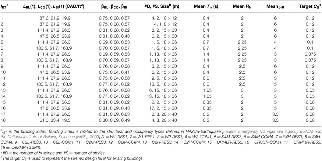
Table 2. Damage cost information (Goda and Hong, 2008b) and considered portfolio of buildings for downtown Vancouver.
Figure 2 shows the comparison between response spectra based on 100 simulation cycles of the simulation in this study with that estimated by Atkinson and Macias (2009) for (49.25°N, 123.13°W). The median spectrum for the 100 simulation cycles and the spectra corresponding to 84th and 16th percentile are also included in Figure 2 to illustrate the dispersion due to simulation. The comparison indicates an adequate match that justifies the simulation method at a single site.
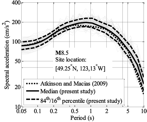
Figure 2. Comparison of the average response spectrum given by Atkinson and Macias (2009) and finite-fault simulations using parameters shown in Tables 1 and 2.
Non-Linear Inelastic 2DOF Systems As Proxy to Buildings and Damage Index
If a building is approximated by a non-linear inelastic SDOF system with Bouc–Wen hysteretic model under unidirectional excitations as was done in Liu and Hong (2015a), the governing equation is expressed in the following using the normalized displacement:
where , μ and μz are the displacement and hysteretic displacement normalized by the yield displacement capacity of the inelastic SDOF system, ΔY (i.e., μ = u/ΔY and μz = z/ΔY, in which u and z are the displacement and hysteretic displacement of the SDOF system, respectively); ωn = (k/m)0.5 is the natural vibration frequency, in which k and m are the stiffness and mass of the system; üg(t) is the ground acceleration time history; εn is the normalized dissipated energy through hysteresis; α, β, γ, and n are shape parameters in which β + γ = 1, α controls the post-yield stiffness, and n controls the smoothness of the transition from linear elastic to non-linear inelastic responses; δη and δv are stiffness and strength degradation parameters, respectively. The defined symbols with additional subscript x are used to denote that they represent the quantities associated with X-axis; and an overdot on a variable denotes its temporal derivative.
The yield displacement ΔY of the non-linear inelastic model could be approximately related to the seismic design requirements (NRCC, 2005), where the minimum required design base shear force Vd is given by Vd = Cs W, W is the total weight of the structure and Cs is the design base shear coefficient given in Table 2 for different building types. It can be shown that ΔY is
where RN is the coefficient taking into account that the actual yield strength of a designed structure is greater than Vd. μR and RN are considered to be lognormally distributed with mean values shown in Table 2 and coefficient of variation (cov) of 0.3 and 0.15 (Ellingwood et al., 1980; Ibarra, 2003), respectively. μR and RN are assumed to be independent for each building.
As mentioned in the Section “Introduction,” the use of the non-linear inelastic 2DOF system to represent a building is more realistic than the use of SDOF system, especially if bidirectional horizontal ground motions are considered. In such a case, the governing equation in terms of normalized displacements can be represented by Park et al. (1986), Yeh and Wen (1990), Lee and Hong (2010):
where , , and the symbols defined previously but with an additional subscript y instead of x represents the quantities associated with the Y -axis. The solution of Eq. 8 can be used to evaluate the “normalized” displacement at time t,
At the incipient yield, max(μD(t)) equals to 1.0; max(μD (t)) represents the peak ductility demand if it is greater than 1.0. By considering that the ductility capacity equals μcap, collapse occurs if max(μD (t)) is greater than μcap. Based on these consideration, for simplicity and being similar to the case of nonlinear inelastic SDOF system (Goda and Hong, 2008b), a damage factor is defined by using,
where . If δDF equals 0, it implies the responses is within elastic range (or at most at incipient yield). Collapse is observed if δDF = 1.0, and partial damage occurs for δDF within (0, 1).
Aggregate Seismic Loss for a Portfolio of Buildings
One of the most difficult and important task in estimating seismic loss is to establish the damage cost function in terms of the damage level (e.g., in terms of damage factor defined in the previous section). This can be carried out if sufficient damage survey data from historical earthquakes are available. However, as the data are always scarce, the damage cost function is often established based on structural component testing results and expert opinion or judgment. A significant set of cost functions is available in HAZUS [Federal Emergency Management Agency (FEMA) and the National Institute of Building Sciences (NIBS), 2003]. These functions for several structural types and in terms of Canadian dollars are given in Goda and Hong (2008b). More specifically, it is considered that seismic losses associated with a building are categorized into three types: building-related loss LBL (δ), contents-related loss LCO(δ), and business-interruption related loss LBI(δ), where δ = δDF. These damage-loss functions can be expressed as,
where the values of losses for the complete damage LBL(1), LCO(1), and LBI(1), as well as the model parameters βBL, βCO, and βBI are shown in Table 2 for each building type. By using the damage-loss functions, the aggregate seismic loss L for nR buildings subjected to the scenario earthquake is calculated using:
where δj denotes the damage factor δDF for the j-th building. The maximum possible aggregate loss, Lmax, equals that calculated from Eq. 12 for δj = 1.
Numerical Example Application in Seismic Loss Estimation
In this section, an example application of the framework shown in the previous section is presented for a scenario seismic event and a portfolio of buildings. For the numerical analysis, the scenario seismic event of moment magnitude M8.5 elaborated previously is considered. The selection of hypothetical portfolio of 100 buildings as well as the analysis results are discussed in the following. Comparison of the aggregate seismic loss of the portfolio of buildings obtained under bidirectional excitations are compared with that obtained by considering unidirectional excitation.
Considered Portfolio of 100 Buildings
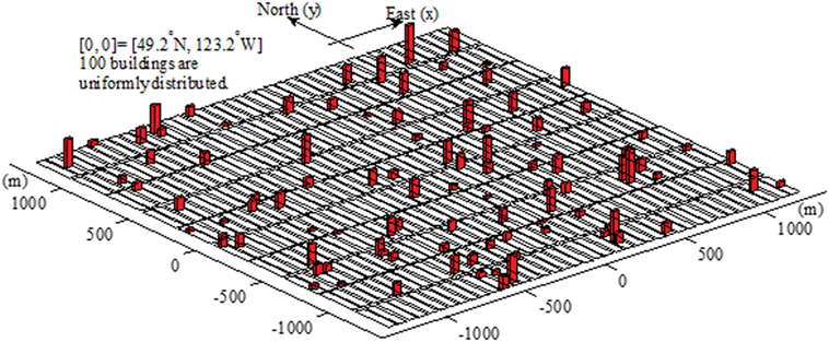
A portfolio of 100 hypothetical buildings located in downtown Vancouver is considered for the numerical example. The sites of the buildings are randomly selected over a square area of 2.5 km by 2.5 km centered at (49.2°N, 123.2°W), which contains 4,000 property lots, each with an area of 25 m × 50 m. The selected locations are illustrated in Figure 3. Similar to Liu and Hong (2015a), the set of 100 buildings consists of 18 building types shown in Table 2. The buildings are of different structural types and occupancies (40 residential buildings and 60 commercial buildings). They are sampled based on the statistical information describing the existing building stocks in downtown Vancouver (Munich Reinsurance Company of Canada, 1992; Onur, 2001). As explained previously, the ductility capacity μcap is considered to be lognormally distributed with cov of 0.3. The mean of the ductility capacity for different building types are shown in Table 2. However, unlike the case in Liu and Hong (2015a), in this study, the capacities of a building in two orthogonal horizontal orientations (i.e., along X-axis and Y -axis) rather than in a single orientation are considered. The yield displacements ΔYx and ΔYx of each building are defined according to Eq. 7, which can be written as with Tn denote the natural vibration period. For each structure, Tn in two orthogonal directions are considered to be independent identically uniformly distributed with mean shown in Table 2 and lower and upper bounds equal to minus and plus 10% of the mean value. This is to represent the fact that the Tn along two horizontal orthogonal direction may differ. RN is considered to be independently lognormally distributed with mean shown in Table 2, and cov equal to 0.15 as discussed previously. Only a single set of structural characteristics of the buildings are sampled and considered in the following numerical analysis.
Illustration of Simulated Ground Motion Components, Calculated Structural Responses, and Damage Cost
For the 100 building sites marked on Figure 3, samples of simulated time histories for two building sites obtained by applying the procedure outlined in the previous section are presented in Figure 4. Note that since the adequacy of the adopted simulation procedure for ground motion records to match the target spatial correlation and coherency and FAS are already discussed extensively elsewhere (Hong and Liu, 2014; Liu and Hong, 2015a), they are not repeated in here. By applying these time histories to the buildings modeled as nonlinear inelastic 2DOF systems, the responses from the time history analysis is shown in Figure 5 in terms of the normalized displacements μx, μy, and μD. The peak values for the normalized displacement and their corresponding time are also shown in the figure. The figure illustrates that the occurrence of peak demand along different component could differ. The total displacement demand μD is greater than a single component.
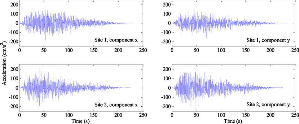
Figure 4. Illustration of simulated spatially correlated and coherent records for two selected sites.
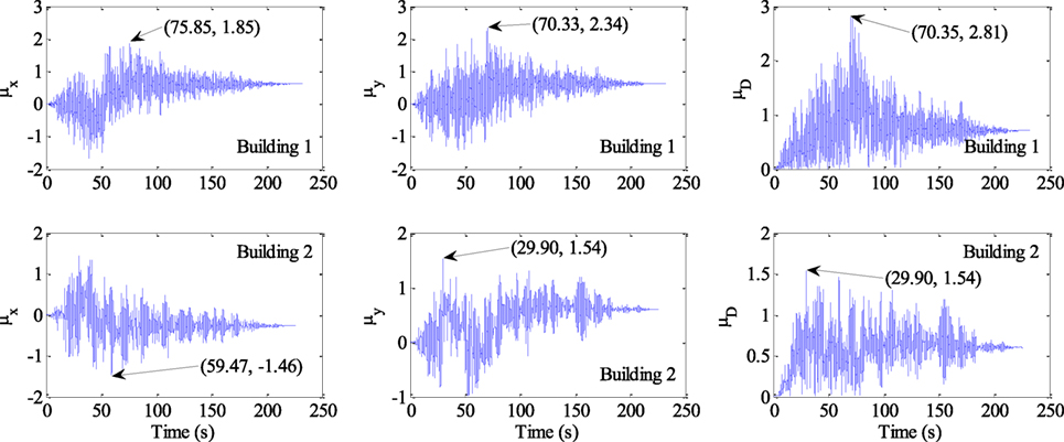
Figure 5. Nonlinear inelastic response of the buildings modeled as 2-degree-of-freedom systems, in terms of normalized displacement response μx, μy, and μD, under the bidirectional ground motions shown in Figure 4. The peak normalized displacement and its corresponding time is also shown.
Based on the non-linear inelastic response, the damage factor of the 2DOF system can be evaluated using Eq. 10. For the two examples given in Figure 5, Building 1 is a 2-story wood frame residential building (Tnx = 0.366 s; Tny = 0.432 s); Building 2 is a 15-story reinforced concrete commercial building (Tnx = 1.664 s; Tny = 1.552 s). The calculated damage factor, δDF = 0.0475 for Building 1 and δDF = 0.554 for Building 2.
Estimation of the Aggregate Loss
The numerical calculation carried out in the previous section is repeated for all 100 considered building. Using the calculated damage cost for each of the 100 buildings, LBL(δ), LCO(δ), and LBI(δ), and summing them up according to Eq. 10, the value of the aggregate loss of the portfolio of buildings L is obtained. This obtained value represents a sample of the aggregate loss for the considered scenario seismic event because of the uncertainty in the ground motions even for the same scenario event. By repeating the above analysis 100 times for the same set of buildings, samples of L are obtained and shown in Figure 6.
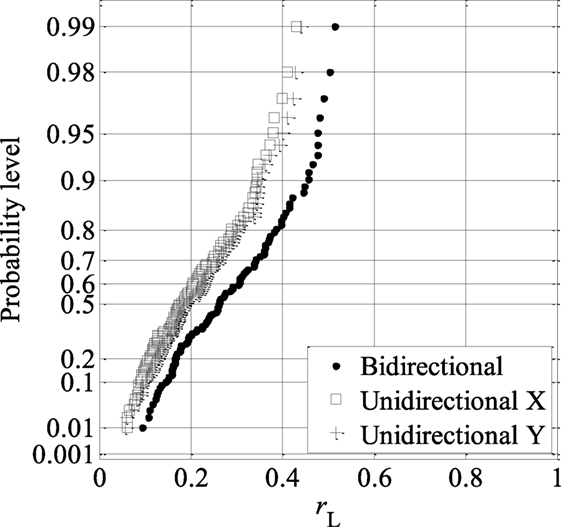
Figure 6. Aggregated seismic loss for the 100 buildings under the scenario earthquake plotted on Gumbel probability paper.
The figure shows that the aggregated seismic loss for the 2DOF system is generally following a straight line on the Gumbel probability paper, with median equal to 0.26.
Effect of Approximating Building As SDOF Systems versus 2DOF Systems
Now, reconsider the ground motions and the structures shown in Figure 3 but only considering the excitations along the X-axis and the buildings modeled as SDOF with the structural properties along the X-axis as well. The calculated responses, the damage factors, and the damage cost for the two buildings are shown in Figure 7. Comparison of the results with those shown in Figure 5 indicate that the profile of the response time history of a SDOF system is generally similar with that of a 2DOF system along the same direction. However, the maximum response could differ significantly because of the consideration of interactions between the two orthogonal directions.
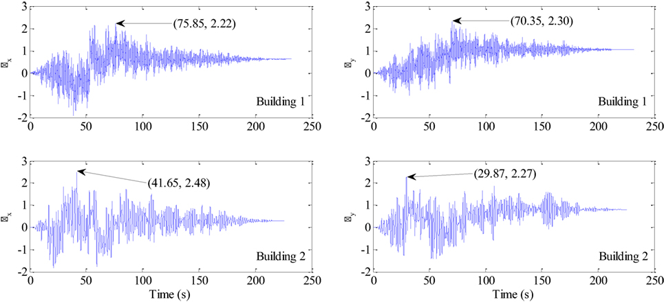
Figure 7. Non-linear inelastic response of the buildings modeled as single-degree-of-freedom systems, in terms of normalized displacement response μx and μy, under the unidirectional ground motions shown in Figure 4. The peak normalized displacement and its corresponding time is also shown.
By repeating the analysis for the building modeled as SDOF systems and subjected to the same set of excitations along the X-axis used in 2DOF system case, samples of L are obtained and also presented in Figure 6. The results follow Gumbel distribution well with a median value of 0.18. Similar analysis is also carried out for Y -axis; the results are also plotted in Figure 6.
Comparison of the results for SDOF systems under unidirectional excitations versus 2DOF systems subjected to bidirectional excitations indicate that the simplification of using unidirectional excitations and SDOF models can underestimate the aggregated seismic loss in a scenario earthquake event. Such underestimation is somewhat more significant at upper tail where the probability of exceedance is small. This observation emphasizes that the importance of using properly simulated bidirectional ground motion excitations and realistic 2DOF structural models in the seismic risk assessment of structures that are sensitive to the orientation of the excitations.
Conclusion
In this study, we first simulate bidirectional spatially (partially) correlated and (partially) coherent ground motion records for a scenario Cascadia earthquake using a simulation procedure based on stochastic finite-fault model. The seismic loss of a portfolio of hypothetical buildings in downtown Vancouver under the simulated bidirectional horizontal ground motions is then estimated. Each building is modeled as a 2DOF system with different dynamic characteristics in two orthogonal horizontal directions. The hysteretic behaviors of the 2DOF systems are described by bidirectional Bouc–Wen model. The results indicate that if unidirectional ground motions and SDOF structural models are considered, the aggregated seismic loss could be underestimated, emphasizing the importance of using realistic bidirectional ground motions that includes spatial coherency and correlation structure and modeling buildings as 2DOF systems with different characteristics in two horizontal directions. If the computation power is not limited, the framework presented in this study can be expanded to investigate the effect of tri-directional ground motions and more complicated structural models.
Author Contributions
TL carried out the analysis and wrote the manuscript. HH oversaw the project and revised the manuscript.
Conflict of Interest Statement
The authors declare that the research was conducted in the absence of any commercial or financial relationships that could be construed as a potential conflict of interest.
Funding
The financial support received from the Natural Sciences and Engineering Research Council of Canada and the University of Western Ontario is gratefully acknowledged.
References
Abrahamson, N. A., Schneider, J. F., and Stepp, J. C. (1991). Spatial coherency of shear waves from the Lotung, Taiwan large-scale seismic test. Struct. Saf. 10, 145–162. doi: 10.1016/0167-4730(91)90011-W
Atkinson, G. M., Assatourians, K., Boore, D. M., Campbell, K., and Motazedian, D. (2009). A guide to differences between stochastic point-source and stochastic finite-fault simulations. Bull. Seism. Soc. Am. 99, 3192–3201. doi:10.1785/0120090058
Atkinson, G. M., and Macias, M. (2009). Predicted ground motions for great interface earthquakes in the Cascadia subduction zone. Bull. Seism. Soc. Am. 99, 1552–1578. doi:10.1785/0120080147
Bazzurro, P., and Cornell, C. A. (1999). Disaggregation of seismic hazard. Bull. Seism. Soc. Am. 89, 501–520.
Boore, D. M. (2009). Comparing stochastic point-source and finite-source ground-motion simulations: SMSIM and EXSIM. Bull. Seism. Soc. Am. 99, 3202–3216. doi:10.1785/0120090056
Cassidy, J. F., and Rogers, G. C. (2004). “Variation in ground shaking on the Fraser River delta (Greater Vancouver, Canada) from analysis of moderate earthquakes,” in Proceedings, 13th World Conference on Earthquake Engineering (Vancouver, Canada). Paper No. 1010.
Clough, R. W., and Penzien, J. (2003). Dynamics of Structures. Berkeley, CA: Computers & Structures, Inc.
Der Kiureghian, A. (1996). A coherency model for spatially varying ground motions. Earthq. Eng. Struct. Dynam. 25, 99–111. doi:10.1002/(SICI)1096-9845(199601)25:1<99::AID-EQE540>3.0.CO;2-C
Ellingwood, B. R., Galambos, T. V., MacGregor, J. G., and Cornell, C. A. (1980). Development of a Probability Based Load Criterion for American National Standard A58. Washington, DC: National Bureau of Standards. National Bureau of Standards Special Publication No. 577.
Federal Emergency Management Agency (FEMA) and the National Institute of Building Sciences (NIBS). (2003). HAZUS-Earthquake: Technical Manual. Washington, DC: FEMA and NIBS.
Goda, K., and Hong, H. P. (2008a). Spatial correlation of peak ground motions and response spectra. Bull. Seism. Soc. Am. 98, 354–365. doi:10.1785/0120070078
Goda, K., and Hong, H. P. (2008b). Estimation of seismic loss for spatially distributed buildings. Earthq. Spectra 24, 889–910. doi:10.1193/1.2983654
Harichandran, R. S., and VanMarcke, E. H. (1986). Stochastic variation of earthquake ground motion in space and time. J. Eng. Mech. 112, 154–174. doi:10.1061/(ASCE)0733-9399(1986)112:2(154)
Hong, H. P., Garcia-Soto, A. D., and Gomez, R. (2010). Impact of different earthquake types on the statistics of ductility demand. J. Struct. Eng. 136, 770–780. doi:10.1061/(ASCE)ST.1943-541X.0000177
Hong, H. P., and Goda, K. (2006). A comparison of seismic hazard and risk deaggregation. Bull. Seism. Soc. Am. 96, 2021–2039. doi:10.1785/0120050238
Hong, H. P., and Hong, P. (2007). Assessment of ductility demand and reliability of bilinear single-degree-of-freedom systems under earthquake loading. Can. J. Civil Eng. 34, 1606–1615. doi:10.1139/L07-077
Hong, H. P., and Liu, T. J. (2014). Assessment of coherency for bi-directional horizontal ground motions and its application for simulating multiple-station bidirectional ground motions. Bull. Seism. Soc. Am. 104, 2491–2502. doi:10.1785/0120130241
Ibarra, L. F. (2003). Global Collapses of Frame Structures under Seismic Excitations. Ph.D. thesis, Stanford University, Stanford, CA.
Jayaram, N., and Baker, J. W. (2009). Correlation model for spatially distributed ground-motion intensities. Earthq. Eng. Struct. Dynam. 38, 1687–1708. doi:10.1002/eqe.922
Lee, C. S., and Hong, H. P. (2010). Statistics of inelastic responses of hysteretic systems under bidirectional seismic excitations. Eng. Struct. 32, 2074–2086. doi:10.1016/j.engstruct.2010.03.008
Liu, T. J., Atkinson, G. M., Hong, H. P., and Assatourians, K. (2012). Intraevent spatial correlation characteristics of stochastic finite – fault simulations. Bull. Seism. Soc. Am. 102, 1740–1747. doi:10.1785/0120110266
Liu, T. J., and Hong, H. P. (2013). Simulation of multiple-station ground motions using stochastic point-source method with spatial coherency and correlation characteristics. Bull. Seism. Soc. Am. 103, 1912–1921. doi:10.1785/0120120203
Liu, T. J., and Hong, H. P. (2015a). Application of spatially correlated and coherent records of scenario event to estimate seismic loss of a portfolio of buildings. Earthq. Spectra 31, 2047–2068. doi:10.1193/060513EQS143M
Liu, T. J., and Hong, H. P. (2015b). Simulation of horizontal ground motions with spatial coherency in two orthogonal horizontal directions. J. Earthq. Eng. 19, 752–769. doi:10.1080/13632469.2014.999175
Motazedian, D., and Atkinson, G. M. (2005). Stochastic finite-fault modeling based on a dynamic corner frequency. Bull. Seism. Soc. Am. 95, 995–1010. doi:10.1785/0120030207
Munich Reinsurance Company of Canada. (1992). A Study of the Economic Impact of a Severe Earthquake in the Lower Mainland of British Columbia. Vancouver, Canada: Munich Reinsurance Company of Canada.
Onur, T. (2001). Seismic Risk Assessment in Southwestern British Columbia. Ph.D. thesis, University of British Columbia, Vancouver, Canada.
Park, Y. J., Wen, Y. K., and Ang, A. (1986). Random vibration of hysteretic systems under bi-directional ground motions. Earthq. Eng. Struct. Dyn. 14, 543–557. doi:10.1002/eqe.4290140405
Shinozuka, M., and Jan, C. M. (1972). Digital simulation of random processes and its applications. J. Sound. Vib. 25, 111–128. doi:10.1016/0022-460X(72)90600-1
Shinozuka, M., Yun, C. B., and Seya, H. (1990). Stochastic methods in wind engineering. J. Wind Eng. Indus. Aerodyn. 36, 829–843. doi:10.1016/0167-6105(90)90080-V
Wen, Y. K. (1976). Method for random vibration of hysteretic systems. J. Eng. Mech. Div. 102, 249–263.
Whitman, R. V., Anagnos, T., Kircher, C. A., Lagorio, H. J., Lawson, R. S., and Schneider, P. (1997). Development of a national earthquake loss estimation methodology. Earthq. Spectra 13, 643–661. doi:10.1193/1.1585973
Yeh, C. H., and Wen, Y. K. (1990). Modeling of nonstationary ground motion and analysis of inelastic structural response. Struct. Saf. 8, 281–298. doi:10.1016/0167-4730(90)90046-R
Keywords: seismic risk, ground motion simulation, bidirectional excitation, 2-degree-of-freedom hysteretic model, Cascadia earthquake
Citation: Liu T and Hong H (2017) Estimation of Seismic Loss for a Portfolio of Buildings under Bidirectional Horizontal Ground Motions due to a Scenario Cascadia Event. Front. Built Environ. 3:61. doi: 10.3389/fbuil.2017.00061
Received: 07 June 2017; Accepted: 02 October 2017;
Published: 24 October 2017
Edited by:
Katsuichiro Goda, University of Bristol, United KingdomReviewed by:
Shinichi Matsushima, Kyoto University, JapanAlkis Daskaloudis, Mott MacDonald, United Kingdom
Copyright: © 2017 Liu and Hong. This is an open-access article distributed under the terms of the Creative Commons Attribution License (CC BY). The use, distribution or reproduction in other forums is permitted, provided the original author(s) or licensor are credited and that the original publication in this journal is cited, in accordance with accepted academic practice. No use, distribution or reproduction is permitted which does not comply with these terms.
*Correspondence: Taojun Liu, bGl1dGFvanVuQGhvdG1haWwuY29t
 Taojun Liu
 Hanping Hong3
