Assessing the Capability of Analytical Carbonation Models to Propagate Uncertainties and Spatial Variability of Reinforced Concrete Structures

Most of the approaches for diagnosis or prognosis of deteriorated reinforced concrete (RC) structures are based on two stages: acquiring data (concrete properties, quantitative degradation information) and then predicting the evolution of degradation by using appropriate models. Spatial variability of both properties and degradation processes cannot be neglected in the lifecycle assessment and implies that (i) data should be acquired for a representative part of the concrete surface and (ii) models should be capable of dealing with this variability. However, the assessment and modeling of spatial variability is not a straightforward task particularly when uncertainties affect the measurements or when the number of measurements is limited. The present paper aims at studying the capability of analytical carbonation models to deal with the spatial variability of model inputs in terms of spatial correlation of model outputs. Analytical models are considered herein because they provide practical and usual tools in engineering. This paper focuses on the case of a RC wall exposed to atmospheric carbonation where concrete properties and carbonation depths were measured by destructive techniques at several points over a linear portion of a wall within the framework of the French ANR EVADEOS project. Uncertainties due to experimental devices and procedures are estimated and propagated throughout random field models to account for spatial variability of spatial observations. Correspondence indexes are proposed to rank carbonation models with respect to their ability of reflecting the observed correlation profiles of carbonation depth. It was found that, for the available database, the proposed correspondence index that incorporates uncertainties was useful to assess the capabilities of models to deal with the spatial variability.

Introduction

Reinforced concrete (RC) is a material widely used in the construction of infrastructure and buildings because of its relative low cost and large durability. However, there are some environmental conditions where physical, chemical, and biological deterioration processes reduce significantly its durability and safety (Bastidas-Arteaga et al., 2009; de Larrard et al., 2014; Marquez-Peñaranda et al., 2016). Among these deterioration processes, atmospheric carbonation of RC structures is one of the major causes of depassivation and then corrosion of steel reinforcing rebars (Ann et al., 2010). Carbonation-induced corrosion damage could certainly increase in the future years by the rise of environmental CO₂ concentration inducing additional maintenance costs (IPCC, 2013; de Larrard et al., 2014; Peng and Stewart, 2016; Stewart et al., 2014).

Maintenance strategies of corroding RC structures aim at predicting corrosion and planning repair operations (coating, replacement of concrete cover, cathodic protection, etc.) in order to maintain acceptable serviceability and safety levels. For new or non-corroded structures, inspection, and data collection are crucial to characterize parameters of carbonation models. The inherent spatial variability of concrete properties and cover depth is of prime importance and must be properly characterized and modeled (Li, 2004; Stewart and Mullard, 2007; Peng and Stewart, 2014); it implies that models must be selected, on the one hand, for representing the carbonation process and predicting corrosion initiation. On the other hand, models must be capable of integrating the spatial variability of input and propagating it onto the output. A convenient way to characterize the spatial variability of stationary random fields is to assess the spatial correlation of data (Schoefs et al., 2009, 2016; O’Connor and Kenshel, 2013; Pasqualini et al., 2013). Knowing the spatial correlation before inspection helps to define an optimal inspection by reducing inspection cost and increasing the predictions accuracy (Bastidas-Arteaga and Schoefs, 2012; O’Connor et al., 2013; Gomez-Cardenas et al., 2015). Inspection or repair decision-making can be efficiently conducted in a probabilistic context especially when statistical and spatial variability of data have been characterized (Stewart, 2004, 2006; Papakonstantinou and Shinozuka, 2013). Data collected from real structures can be perturbed by: spatial variability, measurement error, inaccuracy of experimental devices, complexity of experimental process, etc. Therefore, a dedicated treatment is often applied to data in order to discard gross outliers. In addition, it is not possible to generalize outcomes regarding spatial variability between structures even for the same material property. For instance, concrete mix, execution, and environmental conditions have an important impact on the concrete porosity, and then, the spatial variability of porosity between two components supposedly casted with the same concrete is not necessarily the same. This issue was addressed within the framework of the ANR-EVADEOS project (funded by the French National Research Agency) where a wide experimental investigation was undertaken on several RC structures. Destructive and non-destructive evaluations (NDE) were performed to estimate durability properties of concrete as well as carbonation depth. Only results of destructive tests are considered in this paper. Measurements were taken over a representative part of a concrete wall.

The main objective of the present study is to the estimate the ability of analytical carbonation models to propagate the spatial variability of measured inputs (porosity and saturation degree). The method relies on a comparison between simulated and measured outputs (carbonation depth). A peculiar attention is paid to the quality of data. The effect of gross outliers on the correlation profile of concrete properties is hence studied as well as the influence of unintended deviations in experimental measurements. Moreover, a statistical approach is proposed to study the capability of analytical models to deal with the spatial variability. Section “Investigated Structure” presents the studied structure and the data collected in one experimental investigation of the ANR-EVADEOS Project. Section “Simulation of Random Fields” introduces the computational tools used to assess the correlation profiles and to simulate stationary random fields. We evaluate in Section “Uncertainties from Data and Computation” the uncertainties related to experimental measures. Finally, we propose in Section “Metrics for Estimating the Quality of the Spatial Variability Predictions” various metrics used to evaluate and compare the capability of analytical models to deal with spatial variability.

Investigated Structure

The structure investigated is a concrete wall (Figure 1) built in 1979 enclosing a yard where inert wastes are stored. From carbonation point of view, the exposed surface of the wall represents perfectly a vertical surface of a bridge girder or a column and can be investigated with a lower cost. However, the wall is not cyclically loaded. If the structure was subjected to external mechanical loading, two cases may occur: (i) the loading causes significant mechanical degradation (excessive cracking on given zones for instance): the concrete is hence subjected to substantial supplementary heterogeneity and, therefore, the methodology could not be applied due to the non-stationarity of random fields; (ii) the loading causes negligible or uniform degradation: the results presented in the following would not be affected. The wall is 2.3 m high, several tens of meters long, and 20 cm width. The portion of wall considered is East–West oriented and 3.5 m length. Non-destructive and destructive measurements were carried out on the North face while only destructive measurements were carried out on the South face. The 21 successive measurements along a single horizontal line situated at 1.5 m above the ground were located at center of the reinforcement meshes with a constant distance of 16 cm between measurements. These are common operational conditions: limited number of semi-destructive tests or small distance between tests to ensure the condition of similar exposure zone. It was shown that second order statistical properties of the random filed could be characterized from a single sample function (or trajectory) when using NDEs on similar exposure zones (Schoefs et al., 2016). Concrete saturation degree and porosity were estimated by both destructive and non-destructive techniques. For the destructive tests, cores were extracted according to EN-13791 (2007), porosity and density were determined following the procedure described by NF 18-459 (2010). The distance of the measurement line to the ground (1.5 m) and to the top (0.8 m) was selected to avoid edge effects both from environmental conditions and material variability due to concreting. Compressive strength was estimated by non-destructive techniques (rebound hammer). After inspection, carbonation depth was estimated from extracted cores immediately placed into sealed plastic bags and measurements were conducted in lab.

FIGURE 1

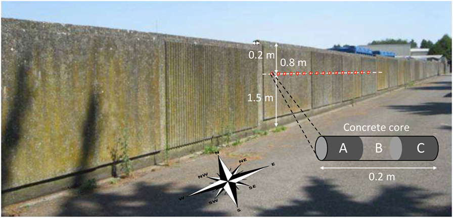
Figure 1. Investigated reinforced concrete wall built in 1979.

Non-destructive evaluation of the same parameters results from a procedure combining different non-destructive technics (ultrasonic waves, radar, impact echo, surface waves, and capacitive sound) by data fusion. This technique was adapted because any of these NDEs can provide a direct measurement of the quantities of interest. Data fusion is based on possibility and fuzzy set theories (Dubois and Prade, 2001). Nevertheless, the assessment of uncertainties affecting the output of the NDEs cannot be easily and directly determined from the observations (frequency, wave velocity, etc.), and European standards do not address this topic yet. Since we want to analyze the capacity of models to propagate uncertainties and spatial variability, NDEs are, therefore, not considered in this paper.

Exposure conditions after 35 years of each wall face are rather different and, consequently, their effect on measured quantities (carbonation depth or saturation degree) is not negligible: on the South side, the drying is faster and the carbonation is supposed to be accelerated. The results indicate (Tables 1 and 2) that the mean value of carbonation depth is 1.96 cm for North side (Side A) and 2.42 cm for South side (Side C). It was, therefore, decided to analyze separately the measurements obtained on each face.

TABLE 1

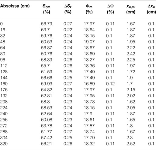
Table 1. Mean values of the measurements and related uncertainties of the saturation degree S_r, porosity Φ, and carbonation depth x_c for the side A.

TABLE 2

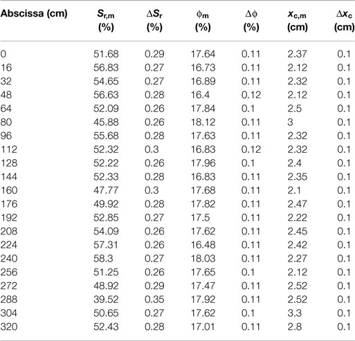
Table 2. Mean values of the measurements and related uncertainties of the saturation degree S_r, porosity Φ, and carbonation depth x_c for the side C.

Simulation of Random Fields

This paper will focus on modeling spatial variability of three properties: concrete saturation degree, porosity and carbonation depth. Given that many studies have been devoted to numerical simulation of random fields—e.g., Kenshel (2009) and Schoefs et al. (2009), this work employs well-known numerical methods toward this aim.

A random field X(x, ω) is a set of random variables X(ω) (where ω denotes hazard) indexed by a parameter x (continuous or discrete) whose values belong to R_n. In this case, x represents the space in the horizontal direction. For a given realization ω₀, X(x, ω₀) represents a sample function (or trajectory) of the random field. This study assumes that the field is ergodic (stationary) to be able to estimate all properties of X(x, ω) (mean, variance, correlation length, statistical moments) from a unique sample function X(x, ω_i). We thus consider only one sample function for each field in the following and ω is not mentioned anymore. For each x₀, X(x₀) is a random variable whose probability density function is $f_{X\left(x_0\right)}\left(h\right)$. The n-order spatial moment $m_D^n$ and the global statistical moment $m_{x_0}^n$ are respectively defined as:

$m_D^n=\begin{array}{c}\lim \\ \left|D\right|\to \infty \\ \end{array}\frac{1}{\left|D\right|}\underset{D}{\int }{X}^n\left(x_0\right)\text{dx}$ (1)

$m_{x_0}^n=E\left[X^n\left(x_0\right)\right]=\underset{\mathfrak{R}}{\int }{X}^n\left(x_0\right)f_{X\left(x_0\right)}\left(h\right)\text{dh}$ (2)

where D describes the geometry of the field and $\mathfrak{R}$ is the space of real numbers. In the case where $m_{X_0}^n$ and $f_{X\left(x_0\right)}\left(h\right)$ do not depend on x₀, the random field is stationary (Property P1). On the other hand, when $m_D^n$ and $m_{X_0}^n$ are equal, the random field is ergodic (Property P2): an ergodic field is thus stationary. Moreover, if the spatial variance $m_D^2$ is also equal to the global statistical variance $m_{X_0}^2$, the random field is second order stationary (Property P3). In this case, the autocorrelation function ρ(x − x′) [correlation between random variables X(x, ω) and X(x′, ω)] depends only on the lag distance Δx = x − x′between two positions x and x′.

Due to the fact that only one realization of each random field is available and for the sake of simplicity, we assume that the random fields are ergodic (P2) and Gaussian. However, additional experimental observations are required to confirm this assumption. Moreover considering more complex type of random fields (non-stationarity or piecewise stationarity) (Schoefs et al., 2009) is beyond the scope of this study and would complicate the comparison between models. That is the case for excessive cracking on given zones. For many practical cases in civil engineering, the amount of data is insufficient to justify or use P1 and we assume P3 (second-order stationarity).

The autocorrelation function of a stationary random field describes the decay of the correlation with respect to the distance between points. Many autocorrelation functions were proposed in the literature [see, for instance, Sudret and Der Kiureghian (2000) and Kenshel (2009) for an overview]. These functions are characterized by the scale fluctuation θ.

Two main procedures are reported in the literature for the estimation of θ. The Maximum Likelihood Estimate method consists in searching for the value of θ that maximizes the joint probability density of the data, supposed to be the realizations of the same distribution function (Li, 2004). Initially correlated according to the ongoing value of θ, these realizations must be transformed into uncorrelated variables so as to compute the joint probability density as a simple product of independent standardized Gaussian variables. The fitting method aims at assessing θ that best fits the correlation profile ρ_D(Δx) obtained from the measured data (Vanmarcke, 1983). For a one dimensional and stationary random field, the correlation profile along the domain is determined as the successive values of the correlation coefficient with respect to the distance Δx between points:

${\mathrm{\rho }}_D\left(\mathrm{\Delta }x\right)={\displaystyle \sum _{i=1}^m}\left[\left(X\left(x_i\right)-m_X\right)\left(X\left(x_i+\mathrm{\Delta }x\right)-m_X\right)\right]$ (3)

where m_X and s_X are, respectively, the mean and SD of X estimated from independent values of data and m is the number of points at a distance Δx from each other.

Among other possible techniques (Lévy, 1965; Vanmarcke, 1983), the Karhunen–Loève expansion (Karhunen, 1947; Lévy, 1965) was used in this study to simulate a Gaussian stationary random field:

$X\left(x,\mathrm{\theta }\right)=m_X+s_X{\displaystyle \sum _{i=1}^n}\sqrt{{\mathrm{\lambda }}_i}{\mathrm{\xi }}_i{f}_i\left(x\right)$ (4)

where n is number of terms in the truncated expansion, ξ_i is a standardized Gaussian random variable, λ_i and f_i are, respectively, the eigenvalues and eigen-functions of the autocorrelation function ρ_D(Δx).

Only few papers in the literature recommend the use of a given autocorrelation function. We propose, herein, to use an exponential autocorrelation function, generally used for representing the autocorrelation of concrete property or durability indicators (Kenshel, 2009; Schoefs et al., 2016). Figure 2B shows that it is well adapted in the present case also. In the case of an exponential autocorrelation function ρ(Δx) = exp(−|Δx|/b) that depends on the correlation parameter b, the eigenvalues λ_i, and eigen-functions f_i are expressed under the assumption that the field is second-order stationarity (Sudret and Der Kiureghian, 2000):

${\mathrm{\lambda }}_i=\frac{2}{b\left(\frac{1}{b^2}+{\mathrm{\omega }}_i^2\right)}$ (5)

$f_i\left(x\right)=\left\{\begin{array}{cc}\frac{\cos \left({\mathrm{\omega }}_{i}x\right)}{\sqrt{a_0+\frac{\sin \left(2{\mathrm{\omega }}_i{a}_0\right)}{2{\mathrm{\omega }}_i}}}& \begin{array}{ccc}\text{for}& i& \text{odd}\end{array}\\ \frac{\sin \left({\mathrm{\omega }}_{i}x\right)}{\sqrt{a_0-\frac{\sin \left(2{\mathrm{\omega }}_i{a}_0\right)}{2{\mathrm{\omega }}_i}}}& \begin{array}{ccc}\text{for}& i& \text{even}\end{array}\end{array}\right.$ (6)

where a₀ is half the length of the domain and ω_i is the solution of the following transcendental equations:

$\left\{\begin{array}{c}\begin{array}{ccc}\hfill \frac{1}{b}-\mathrm{\omega }\tan \left(\mathrm{\omega }{a}_0\right)=0\hfill & \hfill \text{for}\hfill & \hfill \begin{array}{cc}\hfill i\hfill & \hfill \text{odd}\hfill \end{array}\hfill \end{array}\hfill \\ \begin{array}{ccc}\hfill \mathrm{\omega }-\frac{1}{b}\tan \left(\mathrm{\omega }{a}_0\right)=0\hfill & \hfill \text{for}\hfill & \hfill \begin{array}{cc}\hfill i\hfill & \hfill \text{even}\hfill \end{array}\hfill \end{array}\hfill \end{array}\right.$ (7)

FIGURE 2

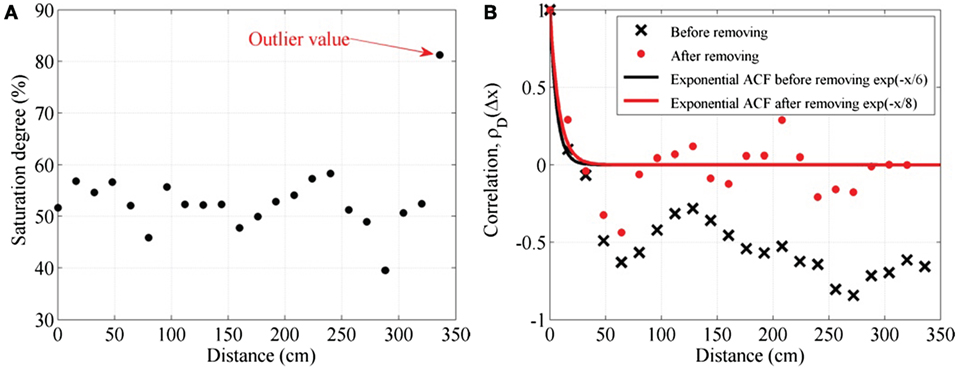
Figure 2. Sample function (A) and spatial correlation profiles (B) of measured saturation degree on the South face of the wall.

Uncertainties from Data and Computation

Uncertainties from Measurements

Four types of uncertainties are described in European standard (AFNOR X07-040-3, 2014):

(i) type A: for a large number of repeated measurements, a statistical treatment allows to express the uncertainty as a function of the SD;

(ii) type B: when only few measurements are available (even only one); other ways can be alternatively employed for assessing the uncertainty in relationship with previous similar measurements, specificity of the device used, error determination of the device, etc.

(iii) combined: a possible combination of the two previous types of uncertainty; and

(iv) expanded standard uncertainties: a combined uncertainty weighted by a coefficient.

Within this study, the experimental parameters affected by uncertainties are those measured once at different locations of the wall from extracted cores: porosity, saturation degree, and carbonation depth. Porosity and saturation degree are estimated as a function f (m_k) of n_m different mass measurements m_k of the core: as such, after complete drying and after complete saturation (mass measured in air or in water). The electronic balance has a known determination error ±Δm and consecutively uncertainty on the mass measurement is $u_m=\mathrm{\Delta }m∕\sqrt{3}$. The uncertainty on the saturation degree or the porosity, u_f, is then expressed as:

$u_f=u_m\sqrt{{\displaystyle \sum _{k=1}^{n_m}}{\left(\frac{\mathrm{\partial f}}{\partial m_k}\right)}^2}$ (8)

The carbonation depth was measured visually with a determination error ±Δx_c depending from the operator. The uncertainty affecting the carbonation depth is then $u_{x_c}=\mathrm{\Delta }{x}_c∕\sqrt{3}$.

Gross Outliers

A primary treatment for the collected data was carried out in order to discard the gross outliers related to particular measurement conditions: the value exceeds the quality requirement [for instance, the discrepancy with other values is greater than three times the SD (Boéro et al., 2009; Pasqualini et al., 2013)], or the value appears to have no physical meaning (for instance, the magnitude of corrosion rate is negative). In case of spatial variability, the spatial evolution of measured values is not chaotic and consecutive values should stay in a given range.

Figure 2A depicts the sample function of measurements of saturation degree from destructive tests on the South face of the wall. It is noted that the value at the abscissa 336 cm is a gross outlier with respect to the values measured in other locations. Accounting for this value in the calculation of the correlation profile leads to significant and meaningless negative values of the correlation coefficient as it can be seen in Figure 2B. Once this value has been removed, the correlation profile seems more relevant although some oscillation remains with still negative values. These negative correlation coefficient values have been also reported when the evaluation is performed with limited data (Pasqualini et al., 2013).

Uncertainty of Assessment for Correlation Coefficient

The correlation profile of data is estimated according to Eq. 3 and its accuracy depends on the number m of couples of measurements available for a distance Δx between points. A larger number of couples reduces the statistical uncertainty. Since repeated values of measurements are used in this work to assess the correlation coefficient of each distance between points, it can be deemed that uncertainty on spatial correlation belongs to type A of uncertainties as described in European Standard. Nevertheless, a direct statistical treatment of spatial correlation is not possible from only one sample function of data. A numerical investigation is hence carried out in order to compute the mean and SD of the correlation coefficient when a large number of sample functions is available and in terms of m.

Using Karhunen–Loeve expansion for an exponential autocorrelation function, n_t = 500 sample functions are simulated for each experimental parameter. Also, n = 100 points of measurements per sample function are generated (the number of points of measurement for each sample function is n = 21 for the experimental data). For each sample function, it is possible to compute a spatial correlation at each distance Δx and therefore to estimate n_t correlation coefficients b with a SD computed as:

${\mathrm{\sigma }}_t\left(\mathrm{\Delta }x\right)=\sqrt{\frac{1}{n_t}{\displaystyle \sum _{i=1}^{n_t}}\left({\mathrm{\rho }}_{D,i}\left(\mathrm{\Delta }x\right)-{\mathrm{\mu }}_t\left(\mathrm{\Delta }x\right)\right)}$ (9)

$\text{with:}{\mathrm{\mu }}_t\left(\mathrm{\Delta }x\right)=\frac{1}{n_t}{\displaystyle \sum _{i=1}^{n_t}}{\mathrm{\rho }}_{D,i}\left(\mathrm{\Delta }x\right)$ (10)

The following procedure was applied to assess how the number m, or indirectly the number of n points in the sample function, impacts the SD σ_t(Δx). For each sample function, the correlation profile is computed considering that a set of n_r points among n is removed from the sample function. All possible sets of n_r points are accounted for, and an average correlation profile is determined for the same sample function. Equations 9 and 10 are then used to compute the mean and SD of ρ_D(Δx) with n–n_r points for all the sample functions. Experimental data are sample functions of 21 points; therefore, the corresponding SDs of ρ_D(Δx) were supplied by removing 79 points from an initial sample function of 100 points. The combined uncertainty on ρ_D(Δx) is then simply $u_{{\mathrm{\rho }}_D\left(\mathrm{\Delta }x\right)}={\mathrm{\sigma }}_t\left(\mathrm{\Delta }x\right)∕\sqrt{m}$.

Metrics for Estimating the Quality of the Spatial Variability Predictions

This section proposes quality indicators to analyze the ability of predictive models to represent the spatial correlation of degradation indicators (carbonation depth). The idea is to quantify how well the spatial correlation of the degradation estimated by the propagation of uncertain measured data through models fits the spatial correlation of the measured degradation. In the aforementioned on-site investigation, each extracted core was divided into three zones, namely, A, B, and C (Figure 1). Sides A and C comprised the edges of the concrete wall exposed to the atmosphere while B was the inner part of the wall. As the carbonation depth is the matter of interest and was not detected on the portion B, only the destructive measurements on sides A and C are considered in this study. The mean values and their related uncertainties are reported in Tables 1 and 2.

Perfect Measurements

Under the assumption of perfect measurements (Schoefs et al., 2009), mean values of measurements reported in Tables 1 and 2 were used as input parameters of the four considered carbonation models: Hyvert (Hyvert et al., 2010); Miragliotta (Miragliotta, 2000); Ying-Yu (Ying-Yu and Qui-Dong, 1987); and Papadakis (Papadakis et al., 1991). Only one sample function of the carbonation depth and subsequent correlation profile were hence computed from each carbonation model (at exposure time t_exp = 35 years) and compared to the correlation profile of the experimental data. Taking into account the lag ε_ρ(Δx_i) between points of the two correlation profiles at the same distance Δx_i (see Figure 3 for the Hyvert model), a normalized scalar metric is proposed as:

$\begin{array}{cc}\hfill I_{\mathit{CM}}=1-\frac{1}{4n}{\displaystyle \sum _{i=1}^n}{\left[{\mathrm{\epsilon }}_{\mathrm{\rho }}\left(\mathrm{\Delta }{x}_i\right)\right]}^2\hfill & \hfill 0\le {\mathrm{\epsilon }}_{\mathrm{\rho }}\left(\mathrm{\Delta }{x}_i\right)\le 2\hfill \\ \hfill \hfill \end{array}$ (11)

FIGURE 3

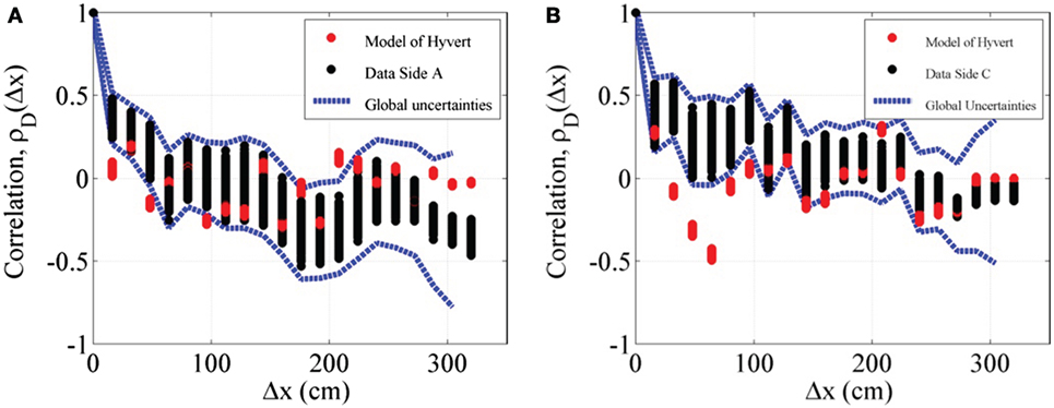
Figure 3. Experimental correlation profiles and profiles obtained by the Hyvert model. (A) Side A. (B) Side C.

Since ρ takes values between −1 and 1, ε_ρ (Δx_i) can vary from 0 (best situation) to 2 (worst situation), the so-called “correspondence index” varies from 0 to 1.

Table 3 provides the ranking of models using this metric. A slight difference appears between the ranking for the sides A and C for Hyvert and Papadakis models. Nevertheless, these results indicate that this metric does not discriminate efficiently the models because all values are close to 0.99.

TABLE 3

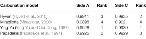
Table 3. Correspondence index for perfect measurement.

Uncertain Measurements

Measurements uncertainty was represented by uniform distributions centered at the measured (mean) values for each investigated point along the wall for the saturation degree and porosity: $S_r\in \lfloor S_{r,m}\pm \mathrm{\Delta }{S}_r\rfloor$ and $\mathrm{\varphi }\in \left[{\mathrm{\varphi }}_m\pm \mathrm{\Delta \varphi }\right]$. Karhunen–Loève expansion was used to simulate 1,000 sample functions of these input parameters that were then used to compute sample functions of carbonation depth at t_exp = 35 years. Similarly, 1,000 sample functions of experimental carbonation depth were directly sampled according to a uniform distribution of x_c, $x_c\in \lfloor x_{c,m}\pm \mathrm{\Delta }{x}_c\rfloor$ centered on experimental data.

Simulated correlation profiles of x_c, ρ_D(Δx), were estimated from these sample functions according to Eq. 3. Figures 3 and 4 illustrate these correlation values for two carbonation models. Uncertainty due to the numerical inaccuracy in the computation of the experimental correlation profiles (see Uncertainty of Assessment for Correlation Coefficient) is also added to the global uncertainties represented by up and down doted lines. It is noted that values corresponding to experimental correlation profiles are more sprayed, for the same lag distance Δx, than those computed from model output. This is due to the fact that the coefficient of variation of the carbonation depth is lower when computed from the rather narrow range of variation of input parameters, than when calculated from experimental carbonation depth. When comparing Figures 3 and 4, it can be seen that this variation depends also on the considered model; for the considered models, the propagation of the same uncertainties of input parameters leads to a wider dispersion for the Papadakis model.

FIGURE 4

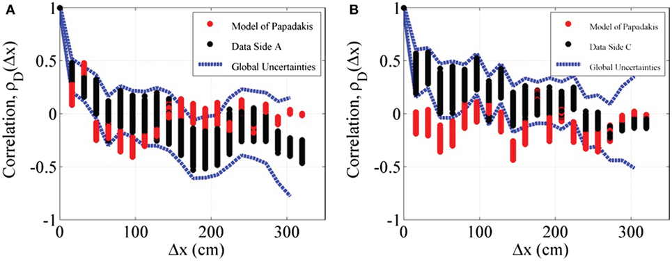
Figure 4. Experimental correlation profiles and profiles obtained by the Papadakis model. (A) Side A. (B) Side C.

From Figures 3 and 4, two correspondence indices can be defined based now on the overlapping of the correlation profiles obtained, respectively, by models and direct assessment. While the first one (I_CM,mes) considers only measurement uncertainty, the second one (I_CM,global) adds global uncertainties. Both indices are estimated according to the following procedure:

1. for each distance Δx_i, let n_mes,i and n_global,i be the number of values of spatial correlations which satisfy to:

$\begin{array}{l}\min \left({\mathrm{\rho }}_{\text{mes,}i}\right)\le {\mathrm{\rho }}_{\text{mod,}i}\le \max \left({\mathrm{\rho }}_{\text{mes,}i}\right)\text{for measurement uncertainty}\\ \min \left({\mathrm{\rho }}_{\text{global,}i}\right)\le {\mathrm{\rho }}_{\text{mod,}i}\le \max \left({\mathrm{\rho }}_{\text{global,}i}\right)\text{for global uncertainty}\end{array}$ (12)

2. if N is the total number of spatial correlation profiles, two correspondence marks could be defined for each distance Δx_i:

$\begin{array}{ll}\hfill \begin{array}{rl}{T}_{\text{mes,}i}& =\frac{n_{\text{mes,}i}}{N}\text{for measurement uncertainty}\\ T_{\text{global,}i}& =\frac{n_{\text{global,}i}}{N}\text{for global uncertainty}\end{array}& \end{array}$ (13)

3. the correspondence indices can be expressed as follows, where n is the number of evaluation points:

$\begin{array}{ll}\hfill \begin{array}{rl}{I}_{\text{CM,mes}}& =\frac{1}{n}{\displaystyle \sum _i^n}{T}_{\text{mes,}i}\text{for measurement uncertainty}\\ I_{\text{CM,global}}& =\frac{1}{n}{\displaystyle \sum _i^n}{T}_{\text{global,}i}\text{for global uncertainty}\end{array}& \end{array}$ (14)

Table 4 summarizes the ranking of the models according to I_CM,mes and I_CM,global. Not surprisingly, the values of I_CM,global, encompassing the effect of numerical inaccuracy in the computation of the correlation coefficients, are larger than those of I_CM,mes. Both indices provide the same ranking for the models for side A. Nevertheless, for the side C, most part of correlation profiles obtained by models are negative whereas those deduced from carbonation depth measurement remain largely positive (Figures 3 and 4). Excepting Ying-Yu (Ying-Yu and Qui-Dong, 1987) model, all the values of I_CM,mes and I_CM,global were significantly reduced meaning that the models are less useful to represent the spatial variability of side C. In comparison with the I_CM metric established without accounting for uncertainties (Eq. 11), it is forth noting that I_CM,mes and I_CM,global are more efficient metrics to discriminate models once uncertainties are accounted for.

TABLE 4

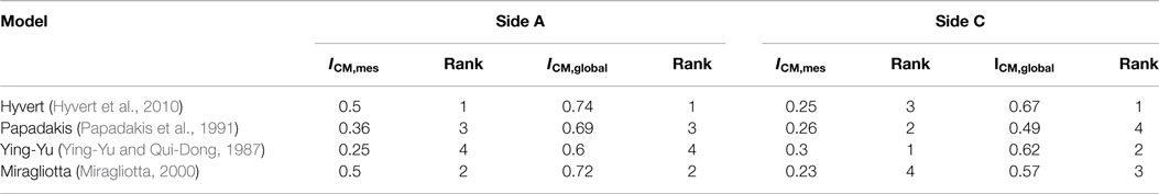
Table 4. Rank of the models according to I_CM,mes and I_CM,global.

According to Table 4, Hyvert model seems to be more appropriate to represent spatial variability, excepting for the side C when numerical inaccuracy for the computation is not considered. Miragliotta model appears also relevant in its capability to transfer the spatial variability for the side A, but it should be discarded for the side C. Due to their exposure to rain, sun, and wind, sides A and C of the wall experienced different behavior regarding carbonation, despite the fact that concrete properties should be the same (concrete pouring was naturally simultaneous for both sides). It seems that exposure effect, combined to the initial spatial variability of concrete properties, considerably modified spatial variability of deterioration processes. It can be deemed in addition that concrete aging is also altered by exposure conditions impacting the initial spatial variability. These considerations could partly explain the discrepancy of the model performance as function of the side considered.

Conclusion

The spatial variability of degradation processes (chlorination, carbonation, depassivation of steel reinforcing bars, etc.) has to be considered for structural inspection, diagnosis, and maintenance. Indeed, when the maintenance strategy is risk-based, which is a global trend nowadays, assessing the probability of depassivation over a global surface of a concrete wall or structure can help to define a portion of that surface presenting a substantial risk and then prescribe appropriate maintenance measures. The probabilistic assessment must be based on a more or less refined knowledge of the spatial correlation existing in concrete cover depth, concrete properties (for instance porosity), and state indicators (for instance saturation degree). Theoretical considerations were developed from decades to represent this spatial variability within the rational framework of the stochastic finite element method. The probabilistic assessment combines these stochastic methods with deterioration (carbonation) models to estimate failure risks. Carbonation models could take more or less complex analytical or numerical forms.

This paper estimated the capability of one-dimension analytical carbonation models to deal with spatial variability based on in-field data. The database contains some input and output model parameters determined from destructive testing on cores extracted from an enclosure wall. The correlation profiles of the carbonation depth either obtained from the measurements or computed thanks to the experimental input used in the models were established. Two normalized so-called correspondence indices were proposed based on (i) the “distance” between profiles for perfect measurements or (ii) the “overlapping” of simulated and experimental data for uncertain measurements. The correspondence index determined without accounting for uncertainties is not relevant in practice because it does not allow the models to be properly discriminated. Contrarily, the correspondence index incorporating uncertainties reveals clearly the various capabilities of models to transfer the spatial variability from input to output, compared to the experimental one. It was found that some models are more or less appropriate to propagate spatial variability depending on the exposure conditions. However, it was not possible to establish a unique ranking from the existing database because carbonation processes were influenced by environmental conditions that differ for each side of the wall. It can be, therefore, concluded that the proposed methodology allows determining the capability of carbonation models to deal with uncertainties and spatial variability as a function of the exposure zone. More experimental data are required for generalization purposes.

Author Contributions

FS: probabilistic modeling of spatial variability, FD: carbonation models, NR: NDT and destructive techniques, TL: numerical simulations, EB-A: propagation of uncertainties through models of degradation.

Conflict of Interest Statement

The authors declare that the research was conducted in the absence of any commercial or financial relationships that could be construed as a potential conflict of interest.

Acknowledgments

Partners of the ANR EVADEOS project are warmly thanked for the data that have been acquired and shared out (CEA Saclay, IFSTTAR Nantes, LMA Univ. Aix-en-Provence, I2M Univ. Bordeaux, EDF Chatou, LMDC Univ. Toulouse, GeM Univ. Nantes).

References

AFNOR X07-040-3. (2014). Uncertainly of Measurement – Part 3: Guide to the Expression of Uncertainly in Measurement (GUM : 1995). Standard. Paris: AFNOR.

Google Scholar

Ann, K. Y., Pack, S.-W., Hwang, J.-P., Song, H.-W., and Kim, S.-H. (2010). Service life prediction of a concrete bridge structure subjected to carbonation. Constr. Build. Mater. 24, 1494–1501. doi: 10.1016/j.conbuildmat.2010.01.023

CrossRef Full Text | Google Scholar

Bastidas-Arteaga, E., Bressolette, P., Chateauneuf, A., and Sánchez-Silva, M. (2009). Probabilistic lifetime assessment of RC structures under coupled corrosion-fatigue processes. Struct. Saf. 31, 84–96. doi:10.1016/j.strusafe.2008.04.001

CrossRef Full Text | Google Scholar

Bastidas-Arteaga, E., and Schoefs, F. (2012). Stochastic improvement of inspection and maintenance of corroding reinforced concrete structures placed in unsaturated environments. Eng. Struct. 41, 50–62. doi:10.1016/j.engstruct.2012.03.011

CrossRef Full Text | Google Scholar

Boéro, J., Schoefs, F., Melchers, R., and Capra, B. (2009). “Statistical analysis of corrosion process along French coast,” in ICOSSAR’09, eds H. Furuta, D. M. Frangopol and M. Shinozuka (Osaka: Taylor & Francis Group), 2226–2233.

Google Scholar

de Larrard, T., Bastidas-Arteaga, E., Duprat, F., and Schoefs, F. (2014). Effects of climate variations and global warming on the durability of RC structures subjected to carbonation. Civil Eng. Environ. Syst. 31, 153–164. doi:10.1080/10286608.2014.913033

CrossRef Full Text | Google Scholar

Dubois, D., and Prade, H. (2001). Possibility theory, probability theory and multiple-valued logics: a clarification. Ann. Math. Artif. Intell. 32, 35–66. doi:10.1023/A:1016740830286

CrossRef Full Text | Google Scholar

EN-13791. (2007). Assessment of In-Situ Compressive Strength in Structures and Pre-Cast Concrete Components. Paris: AFNOR.

Google Scholar

Gomez-Cardenas, C., Sbartaï, Z. M., Balayssac, J. P., Garnier, V., and Breysse, D. (2015). New optimization algorithm for optimal spatial sampling during non-destructive testing of concrete structures. Eng. Struct. 88, 92–99. doi:10.1016/j.engstruct.2015.01.014

CrossRef Full Text | Google Scholar

Hyvert, N., Sellier, A., Duprat, F., Rougeau, P., and Francisco, P. (2010). Dependency of C–S–H carbonation rate on CO2 pressure to explain transition from accelerated tests to natural carbonation. Cem. Concr. Res. 40, 1582–1589. doi:10.1016/j.cemconres.2010.06.010

CrossRef Full Text | Google Scholar

IPCC. (2013). “Climate change 2013: the physical science basis,” in Contribution of Working Group I to the Fifth Assessment Report of the Intergovernmental Panel on Climate Change, eds T. F. Stocker, D. Qin, G.-K. Plattner, M. Tignor, S. K. Allen, J. Boschung, A. Nauels, Y. Xia, V. Bex, and P. M. Midgley (Cambridge, UK; New York, NY, USA: Cambridge University Press), 465–544.

Google Scholar

Karhunen, K. (1947). Uber lineare methoden in der wahrscheinlichkeitsrechnung. Amer. Acad. Sci. 73, 73–79.

Google Scholar

Kenshel, O. (2009). Influence of Spatial Variability on Whole Life Management of Reinforced Concrete Bridges. Dublin, Ireland: University of Dublin, Trinity College.

Google Scholar

Lévy, P. (1965). Processus stochastic et mouvement brownien. Paris: Jacques Gabay.

Google Scholar

Li, Y. (2004). Effect of Spatial Variability on Maintenance and Repair Decisions for Concrete Structures. Delft, Netherlands: Delft University.

Google Scholar

Marquez-Peñaranda, J. F., Sanchez-Silva, M., Husserl, J., and Bastidas-Arteaga, E. (2016). Effects of biodeterioration on the mechanical properties of concrete. Mater. Struct. 49, 4085–4099. doi:10.1617/s11527-015-0774-4

CrossRef Full Text | Google Scholar

Miragliotta, R. (2000). Modélisation des processus physico-chimiques de la carbonatation des bétons préfabriqués : prise en compte des effets de paroi. La Rochelle.

Google Scholar

NF 18-459. (2010). Essai pour béton durci – Essai de porosité et de masse volumique (Tests for Determining Porosity and Density for Hard Concrete).

Google Scholar

O’Connor, A., and Kenshel, O. (2013). Experimental evaluation of the scale of fluctuation for spatial variability modeling of chloride-induced reinforced concrete corrosion. J.Bridge Eng. 18, 3–14. doi:10.1061/(ASCE)BE.1943-5592.0000370

CrossRef Full Text | Google Scholar

O’Connor, A. J., Sheils, E., Breysse, D., and Schoefs, F. (2013). Markovian bridge maintenance planning incorporating corrosion initiation and nonlinear deterioration. J. Bridge Eng. 18, 189–199. doi:10.1061/(ASCE)BE.1943-5592.0000342

CrossRef Full Text | Google Scholar

Papadakis, V. G., Vayenas, C. G., and Fardis, M. N. (1991). Fundamental modeling and experimental investigation of concrete carbonation. Mater. J. 88, 363–373.

Google Scholar

Papakonstantinou, K. G., and Shinozuka, M. (2013). Probabilistic model for steel corrosion in reinforced concrete structures of large dimensions considering crack effects. Eng. Struct. 57, 306–326. doi:10.1016/j.engstruct.2013.06.038

CrossRef Full Text | Google Scholar

Pasqualini, O., Schoefs, F., Chevreuil, M., and Cazuguel, M. (2013). Measurements and statistical analysis of fillet weld geometrical parameters for probabilistic modelling of the fatigue capacity. Mar. Struct. 34, 226–248. doi:10.1016/j.marstruc.2013.10.002

CrossRef Full Text | Google Scholar

Peng, L., and Stewart, M. G. (2014). Spatial time-dependent reliability analysis of corrosion damage to RC structures with climate change. Mag. Concrete Res. 66, 1154–1169. doi:10.1680/macr.14.00098

CrossRef Full Text | Google Scholar

Peng, L., and Stewart, M. G. (2016). Climate change and corrosion damage risks for reinforced concrete infrastructure in China. Struct. Infrastruct. Eng. 12, 499–516. doi:10.1080/15732479.2013.858270

CrossRef Full Text | Google Scholar

Schoefs, F., Bastidas-Arteaga, E., Tran, T. V., Villain, G., and Derobert, X. (2016). Characterization of random fields from NDT measurements: a two stages procedure. Eng. Struct. 111, 312–322. doi:10.1016/j.engstruct.2015.11.041

CrossRef Full Text | Google Scholar

Schoefs, F., Clement, A., and Nouy, A. (2009). Assessment of spatially dependent ROC curves for inspection of random fields of defects. Struct. Saf. 31, 409–419. doi:10.1016/j.strusafe.2009.01.004

CrossRef Full Text | Google Scholar

Stewart, M. G. (2004). Spatial variability of pitting corrosion and its influence on structural fragility and reliability of RC beams in flexure. Struct. Saf. 26, 453–470. doi:10.1016/j.strusafe.2004.03.002

CrossRef Full Text | Google Scholar

Stewart, M. G. (2006). Spatial variability of damage and expected maintenance costs for deteriorating RC structures. Struct. Infrastruct. Eng. 2, 79–96. doi:10.1080/15732470500253230

CrossRef Full Text | Google Scholar

Stewart, M. G., and Mullard, J. A. (2007). Spatial time-dependent reliability analysis of corrosion damage and the timing of first repair for RC structures. Eng. Struct. 29, 1457–1464. doi:10.1016/j.engstruct.2006.09.004

CrossRef Full Text | Google Scholar

Stewart, M. G., Val, D. V., Bastidas-Arteaga, E., O’Connor, A., and Wang, X. (2014). “Climate adaptation engineering and risk-based design and management of infrastructure,” in Maintenance and Safety of Aging Infrastructure, eds D. Frangopol and Y. Tsompanakis (CRC Press), 641–684.

Google Scholar

Sudret, B., and Der Kiureghian, A. (2000). Stochastic Finite Elements and Reliability: A State-of-the-Art Report. Report No: UCB/SEMM-2000/08. Berkeley: Department of Civil & Environmental Engineering – University of California.

Google Scholar

Vanmarcke, E. (1983). Random Fields: Analysis and Synthesis. Cambridge, MA; London: MIT Press.

Google Scholar

Ying-Yu, L., and Qui-Dong, W. (1987). “The mechanism of carbonation of mortars and the dependence of carbonation on pore structure,” in Concrete Durability – Katherine and Bryan Mather International Conference (Detroit: American Concrete Institute), 1915–1943.

Google Scholar