Probabilistic Earthquake–Tsunami Multi-Hazard Analysis: Application to the Tohoku Region, Japan

This study develops a novel simulation-based procedure for the estimation of the likelihood that seismic intensity (in terms of spectral acceleration) and tsunami inundation (in terms of wave height), at a particular location, will exceed given hazard levels. The procedure accounts for a common physical rupture process for shaking and tsunami. Numerous realizations of stochastic slip distributions of earthquakes having different magnitudes are generated using scaling relationships of source parameters for subduction zones and then using a stochastic synthesis method of earthquake slip distribution. Probabilistic characterization of earthquake and tsunami intensity parameters is carried out by evaluating spatially correlated strong motion intensity through the adoption of ground motion prediction equations as a function of magnitude and shortest distance from the rupture plane and by solving non-linear shallow water equations for tsunami wave propagation and inundation. The minimum number of simulations required to obtain stable estimates of seismic and tsunami intensity measures is investigated through a statistical bootstrap analysis. The main output of the proposed procedure is the earthquake–tsunami hazard curves representing, for each mean annual rate of occurrence, the corresponding seismic and inundation tsunami intensity measures. This simulation-based procedure facilitates the earthquake–tsunami hazard deaggregation with respect to magnitude and distance. Results are particularly useful for multi-hazard mapping purposes, and the developed framework can be further extended to probabilistic earthquake–tsunami risk assessment.

Introduction

Earthquake and tsunami can be concurrent threats in many coastal regions around the world. In the last 2500 years, more than 2500 major tsunami events occurred globally (NGDC, 2016), and more than a half of those were triggered by seismic events. Other events were generated by volcanic eruptions (Latter, 1981), submarine landslides (Satake, 2001; Ward, 2001; Watts, 2004), or potentially by asteroid/meteorite impacts (Ward and Asphaug, 2000). Figure 1 shows the distribution of tsunami events triggered by seismic events at a global scale (NGDC, 2016). Tsunamis are particularly likely in active subduction zones surrounding the Pacific and Indian Oceans and are less expected in crustal seismogenic regions surrounding the Mediterranean Sea. Nonetheless, devastating tsunami disasters can occur in the Mediterranean areas, as exemplified by two historical disasters, i.e., the 1303 Crete Island tsunami (Guidoboni and Comastri, 1997) and the 1908 Messina event (Billi et al., 2008). It is therefore evident that simultaneous earthquake–tsunami hazard represents an urgent global issue and may cause catastrophic loss, affecting communities along coastal regions from economic and social viewpoints (Løvholt et al., 2014).

FIGURE 1

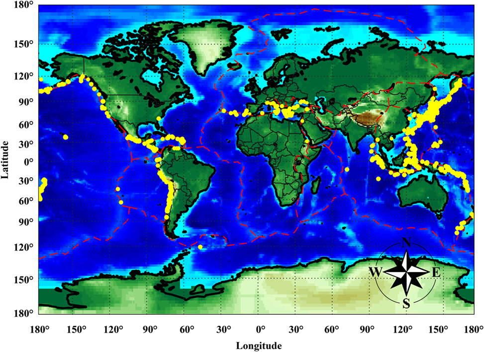
Figure 1. Locations of tsunamis triggered by seismic events. The red lines represent the global plate margins.

Seismic sources close to the shoreline can trigger tsunamis that cause devastating damage, especially due to the lack of sufficient reaction time (Monastersky, 2012). Thus, tsunamis triggered by near-field seismic sources can be regarded as the main contributors of the tsunami risk impact, and they should be studied in detail. Moreover, in comparison to local tsunamis, a simpler parameterization is usually sufficient for far-field tsunamis because seismic moment, source mechanism, and radiation pattern are more influential in comparison with slip distribution within a rupture plane (Geist and Parsons, 2006). For the above reasons, this work will focus on near-field scenarios by considering detailed features of the earthquake rupture.

Probabilistic hazard analysis is the fundamental prerequisite for assessing disaster risk accurately and for deciding effective risk mitigation strategies. Both probabilistic earthquake and tsunami analyses involve various uncertain parameters that are related to geophysical processes and geological characteristics [e.g., slip rate, slip distribution, dip, and strike (Goda et al., 2014)], propagating media, local site conditions (e.g., soil type, roughness, and topography), and sea conditions [e.g., tidal level (Mofjeld et al., 2007)]. Conventional probabilistic seismic hazard analysis [PSHA (Cornell, 1968; McGuire, 2008)] can incorporate all major uncertain parameters in a comprehensive manner, with a potentially high computational effort. The computation becomes prohibitive when a logic tree with numerous branches (to capture full extent of epistemic uncertainty) is adopted for the assessment. In order to reduce this effort, a simulation-based probabilistic procedure can be implemented (Atkinson and Goda, 2013; Akkar and Cheng, 2015).

In the current probabilistic tsunami hazard analysis (PTHA), a comprehensive treatment of these uncertainties is rarely considered due to the lack of high-resolution/accuracy data and to the great computational effort involved in tsunami simulations. There are mainly three methodologies for tsunami hazard assessment in the literature (González et al., 2009): (a) probabilistic hazard analysis; (b) worst-case scenario approach, typically a deterministic method used for the development of practical emergency management products, such as evacuation maps and coastal infrastructure design (Cheung et al., 2011); and (c) sensitivity analysis, where the most influential model parameters are identified (Geist, 2002; Goda et al., 2014). The existing PTHA methods can be grouped in three broad categories. In the first category, PTHA is conducted by using tsunami catalogs (Burroughs and Tebbens, 2005; Tinti et al., 2005; Orfanogiannaki and Papadopoulos, 2007); in the second category, different scenario-based PTHA methods are suggested (Geist and Dmowska, 1999; Downes and Stirling, 2001; Farreras et al., 2007; Liu et al., 2007; Power et al., 2007; Yanagisawa et al., 2007; Burbidge et al., 2008; González et al., 2009; Løvholt et al., 2012). In the third category, a combination of the two previous categories is considered (Geist, 2005; Geist and Parsons, 2006; Annaka et al., 2007; Thio et al., 2007; Burbidge et al., 2008; Parsons and Geist, 2008; Grezio et al., 2010, 2012; Horspool et al., 2014; Fukutani et al., 2016). Specifically, for near-source subduction zones, Fukutani et al. (2016) extended the methodology of Annaka et al. (2007) for a Tohoku-type (M9) earthquake with fixed rupture geometry. They considered several cases for earthquake magnitude, slip pattern, and occurrence probability. However, the numbers of magnitudes and slip patterns are limited and thus not sufficient to capture a wide range of possible tsunami scenarios for this type of mega-thrust subduction earthquakes (Goda et al., 2014).

Building on the previous research, a new probabilistic earthquake and tsunami hazard assessment methodology for near-field seismic sources is presented. The novelty of the proposed methodology is the adoption of a single physical process for concurrent earthquake and tsunami threats; thus, dependency between ground-shaking and tsunami hazard parameters can be investigated probabilistically. On the one hand, the proposed methodology overcomes some of the previous limitations, such as inappropriate scaling relationships, simplistic slip distributions, subjective weights of the logic tree’s branches, and simplified inundation models. On the other hand, some simplification, such as the adoption of discrete values of magnitude, and the fixed geometry and predefined meshing of the main subduction region, are maintained. This methodology can be extended to consider all possible sources in a region and can be applied to other subduction zones.

The first step is to define a suitable occurrence model; classical occurrence models in literature are the memory-less Poisson model, generally used for long-term hazard assessments, and the renewal model [e.g., Brownian passage time model (Matthews et al., 2002)] applied for short-term forecasting based on the seismic activity observed in the recent past. In this study, a classical Poisson model is adopted. Assuming a Poissonian inter-arrival time process, the probability of occurrence of an earthquake–tsunami event with specific characteristics in a given time window depends on the mean annual occurrence rate alone. A magnitude–frequency distribution of major seismic events that may potentially trigger tsunamis is then defined. For each value of earthquake magnitude, geometry of the rupture areas and other key source parameters (mean slip and spatial correlation parameters of slip distribution) are determined using new global scaling relationships for tsunamigenic earthquakes (Goda et al., 2016). In this step, both aleatory and epistemic uncertainties of the model parameters (i.e., position and geometry) are incorporated based on probabilistic information available in literature. Therefore, for each value of magnitude, multiple realizations of potential earthquake slip distribution are generated from a theoretical wavenumber spectrum model (Mai and Beroza, 2002). The incorporation of stochastic slip models in probabilistic earthquake–tsunami hazard analysis is another important novelty of this work with respect to the previous studies; conventionally, the slip distributions within a fault plane are considered as uniform or randomly distributed (without realistic spatial distribution of the slip).

Subsequently, simulations of the two hazard processes, i.e., ground shaking and tsunami, are carried out simultaneously. Specifically, for each slip distribution: (a) spatially correlated strong motion intensity measures are evaluated using ground motion prediction equations (GMPEs) for interface subduction events (Morikawa and Fujiwara, 2013; Abrahamson et al., 2016); and (b) the seafloor vertical displacement is calculated using analytical formulae (Okada, 1985; Tanioka and Satake, 1996), and tsunami simulation is performed by solving non-linear shallow water equations (Goto et al., 1997). By repeating the joint assessment of earthquake–tsunami hazards a sufficient number of times for each magnitude, a sample of spectral accelerations at multiple locations can be obtained by simulating a seismic intensity random field, while maximum tsunami wave heights/velocities can be obtained from tsunami hazard analysis. For each magnitude, the results obtained from the simulations are used to build the complementary cumulative distribution functions (CCDFs) for individual hazards, representing the conditional probability of reaching or exceeding a given intensity value. The CCDFs are provided with a confidence interval around the central estimates.

The site-specific earthquake–tsunami hazard curves can be derived by integrating the earthquake–tsunami simulation results and the magnitude–frequency distribution for the discrete values of magnitude, and by multiplying the result by the occurrence rate of earthquakes from the subduction zone. The result will be a triplet of CCDFs (central estimate and confidence interval curves), representing the mean annual rate of exceedance of specific values of seismic intensity or tsunami hazard parameters. The developed methodology is applied to the Tohoku region of Japan, where the subduction fault plane is well defined and information on regional seismicity is available. Finally, the hazards for a site in Sendai City, Miyagi Prefecture, are calculated.

Methodology

Formulation

The formulation presented herein is aimed at developing the earthquake–tsunami hazard curves for a specific location. Let IM represent the intensity measures of interest, such as spectral acceleration (S_a), inundation height (h), flow velocity (v), flux momentum, and tsunami force. Assuming a Poissonian arrival time process, the probability to observe an earthquake–tsunami sequence having intensity measure values IM equal to or greater than the specific values im in t years is

$P\left(\mathbf{\text{IM}}\ge \mathbf{\text{im}}|t\right)=1-\exp \left[-\lambda \left(\mathbf{\text{IM}}\ge \mathbf{\text{im}}\right)\cdot t\right]$ (1)

where λ(IM ≥ im) is the mean annual rate at which the intensity measures IM will exceed specific values im at a given location. The rate λ(IM ≥ im) can be expressed as a filtered Poisson process [e.g., Parsons and Geist (2008)]:

$\begin{array}{l}\hfill \lambda \left(\mathbf{\text{IM}}\ge \mathbf{\text{im}}\right)=\lambda \left(M\ge M_{\min }\right)\cdot \mathit{\int }P\left(\mathbf{\text{IM}}\ge \mathbf{\text{im}}|\theta \right)\cdot S\left(\mathrm{\theta }|M\right)\cdot f\left(M\right)\cdot \mathit{\text{dM}}\end{array}$ (2)

λ(M ≥ M_min) is the mean annual rate of occurrence of the seismic events with magnitudes greater than the minimum magnitude considered in the magnitude–frequency distribution. P(IM ≥ im|θ) is the probability that the joint intensity measures IM will exceed prescribed values im at a given coastal location for a given set of source parameters θ. S(θ|M) represents the scaling relationships (or prediction models) of the uncertain earthquake source parameters conditioned on the magnitude. f (M) is the magnitude–frequency distribution.

Five phases are defined: Phase 1 – fault model and earthquake occurrence, Phase 2 – source parameter characterization and stochastic slip synthesis, Phase 3 – earthquake simulation, Phase 4 – tsunami simulation, and Phase 5 – development of earthquake–tsunami hazard curves. Detailed descriptions for each of these phases are presented in the following. Figure 2 shows the computational framework of the methodology.

FIGURE 2

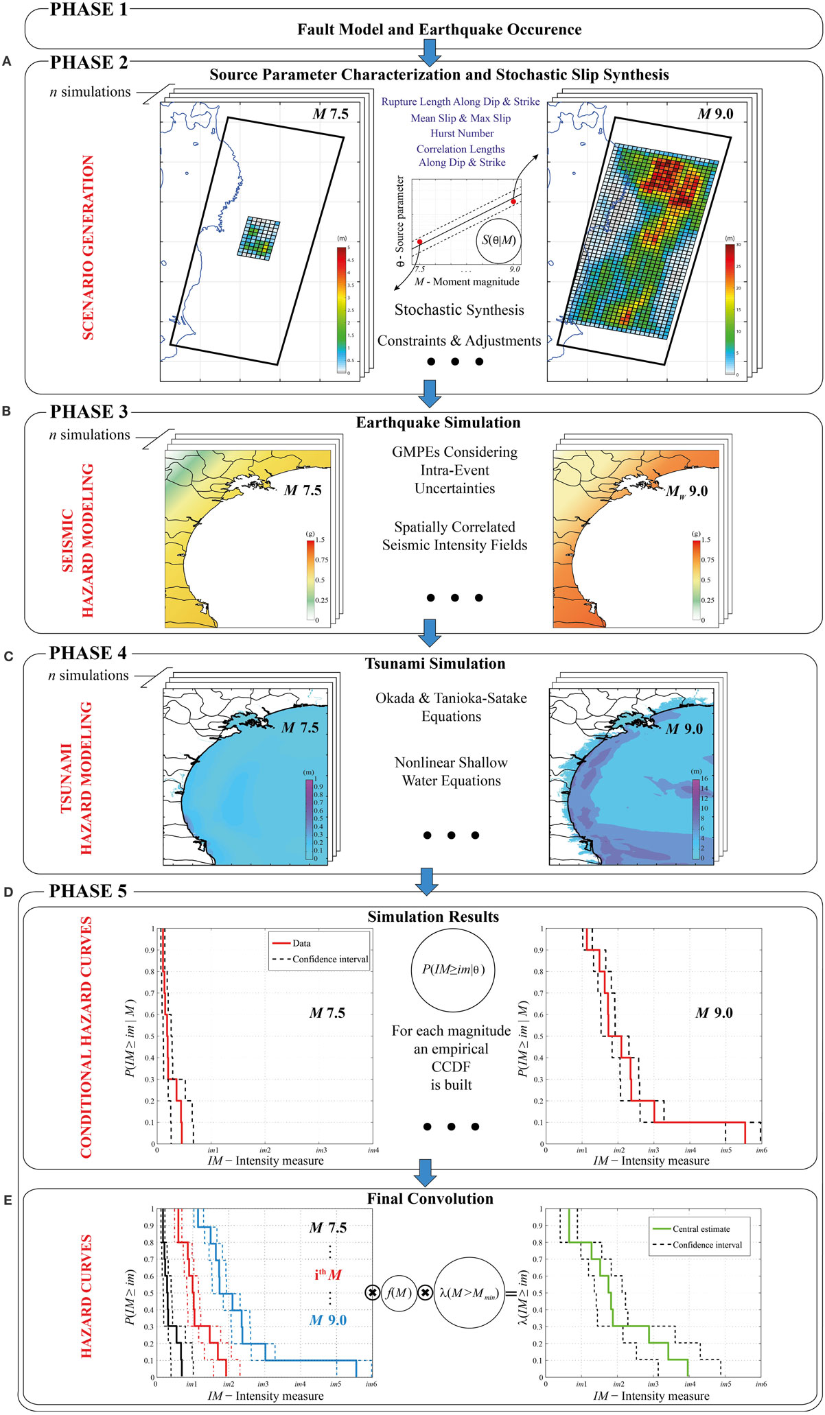
Figure 2. Computational framework for probabilistic earthquake–tsunami hazard analysis. (A) Scenario generation. (B) Seismic hazard modeling. (C) Tsunami hazard modeling. (D) Conditional hazard curves. (E) Hazard curves.

Fault Model and Earthquake Occurrence

The first step is the identification of all seismic sources capable of producing damaging ground motions and tsunami inundation at a site. In this study, a curved surface is considered. Specifically, a 2011 Tohoku-type fault is analyzed with a source zone of 650 km along the strike and 250 km along the dip (Figure 3A); such geometry is capable of accommodating a M9 earthquake that is consistent with the maximum magnitude adopted for the magnitude–frequency distribution. The fault plane geometry is the extended version of the source model by Satake et al. (2013). Note that extremely large earthquakes that span across multiple seismotectonic segments are not considered (e.g., simultaneous rupture of the off-the-Tohoku subduction region and the off-the-Hokkaido subduction zone). To implement the stochastic synthesis method of earthquake slip distribution, the fault plane is discretized into many sub-faults; a 10-km mesh with variable dip based on Satake et al. (2013) is generated. Such a discretization allows simulating accurately the slip distribution corresponding to a seismic event with M7.5 (i.e., the smallest central magnitude value considered for the magnitude–frequency distribution, as shown later), involving at least 5-by-5 sub-faults.

FIGURE 3

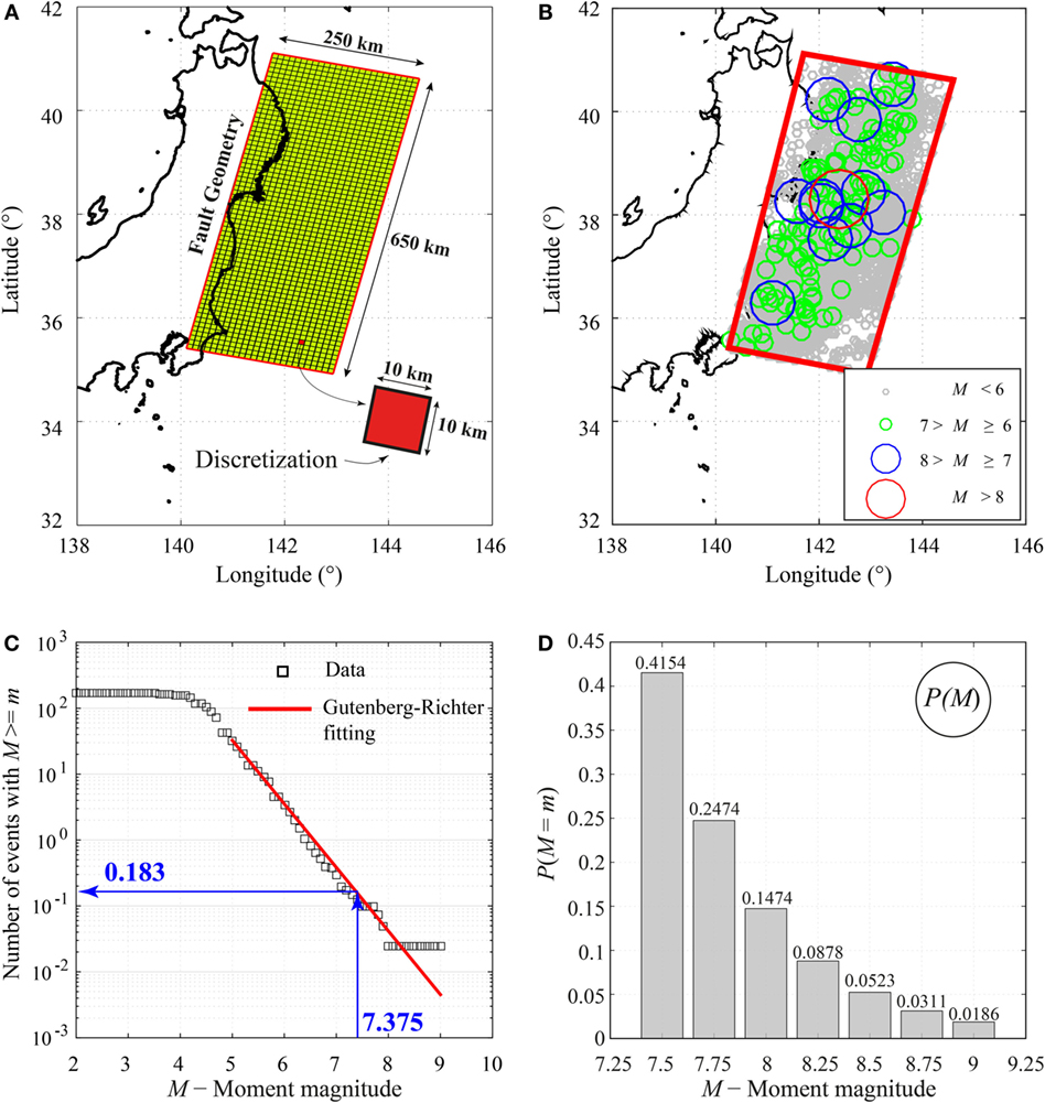
Figure 3. (A) Fault plane model and discretization. (B) Spatial distribution of earthquakes in the source region using the NEIC catalog. (C) Gutenberg–Richter relationship. (D) Discrete probability mass based on the fitted Gutenberg–Richter relationship.

To describe the earthquake sizes in the target region, i.e., the term f (M) in Eq. 2, a truncated Gutenberg–Richter relationship (Gutenberg and Richter, 1956) is adopted, and its CCDF is given by

$G\left(M\right)=\frac{1-{10}^{-b\left(M-M_{\text{min}}\right)}}{1-{10}^{-b\left(M_{\text{max}}-M_{\text{min}}\right)}}{M}_{\text{min}}<M<M_{\text{max}}$ (3)

where M_min and M_max are the minimum and maximum moment magnitudes, respectively. For the simulation, it is convenient to convert the continuous distribution of magnitudes into a discrete set of values (M_min, …, M_i, …, M_max), assuming that they are the only possible magnitudes; such probabilities are computed as follows:

$P\left(M_i\right)=G\left(M_i+0.5\cdot \mathrm{\Delta }M\right)-G\left(M_i-0.5\cdot \mathrm{\Delta }M\right)$ (4)

where ΔM is the discretization interval. The discrete term presented in Eq. 4 is used in Eq. 2 instead of f (M).

For the analyses, M_min and M_max are set to 7.375 and 9.125, and a discretization interval of 0.25 is adopted. This means that seven central magnitude values, i.e., 7.5, 7.75, 8.0, 8.25, 8.5, 8.75, and 9.0, are considered to calculate the corresponding conditional probabilities as in Eq. 4. The minimum magnitude value is chosen, since small-to-moderate earthquakes rarely generate significant tsunamis, and their contributions to the tsunami hazard are negligible (Annaka et al., 2007). For the Tohoku case study, a b-value equal to 0.9 is adopted (Headquarters for Earthquake Research Promotion, 2013).

Once the magnitude interval is selected and the major source area containing all possible rupture scenarios is defined, the mean annual rate of occurrence of earthquakes with magnitudes greater than or equal to 7.375 falling in that area, i.e., the term λ(M ≥ M_min) in Eq. 2, can be calculated. In order to perform such a calculation, the NEIC earthquake catalog (http://earthquake.usgs.gov/earthquakes/search/) is used. Figure 3B shows the events reported in the database that fall in the considered rupture area, recorded in the period between 1976 and 2012, having a depth varying between 0 km and 60 km, and considering a magnitude range between 5 and 9. According to the data analysis (Figure 3C), the estimated rate λ(M ≥ 7.375) is equal to 0.183. Figure 3D shows the occurrence probabilities for the discrete set of magnitude values (i.e., 7.5, 7.75, 8.0, 8.25, 8.5, 8.75, and 9.0). Note that the probability mass function shown in Figure 3D is normalized (conditional) with respect to the occurrence rate for the minimum magnitude event.

Source Parameter Characterization and Stochastic Slip Synthesis

To take into account uncertainties related to the rupture process, multiple random slip fields are simulated (Figure 2A). The simulation procedure is based on a spectral synthesis method (Goda et al., 2014; Fukutani et al., 2016), where the earthquake slip distribution is characterized by wavenumber spectra (Mai and Beroza, 2002; Lavallée et al., 2006). Scaling relationships that evaluate the source parameters as a function of moment magnitude are needed for stochastic tsunami simulation (e.g., rupture size and spectral characteristics of the rupture). In this study, new global scaling relationships for tsunamigenic earthquakes are employed. These relationships are obtained on the basis of 226 inverted source models in the SRCMOD database (Mai and Thingbaijam, 2014). The details of the adopted scaling laws can be found in Goda et al. (2016).

The following relationships are employed to obtain the rupture width (W) and length (L):

${\log }_{10}W=-0.4877+0.3125M+0.1464\times {\mathrm{\epsilon }}_W$ (5)

${\log }_{10}L=-1.5021+0.4669M+0.1717\times {\mathrm{\epsilon }}_L$ (6)

where the numbers multiplying by the ε terms are the SDs of the regression errors. The two geometrical dimensions are used to create the rupture area, which is randomly located inside the predefined subduction fault plane. Subsequently, a slip distribution realization with desired properties is obtained using a stochastic synthesis method (Goda et al., 2014). First, a random field, having quasi-normal distribution with a desired spatial correlation structure, is generated using a Fourier integral method (Pardo-Iguzquiza and Chica-Olmo, 1993). The amplitude spectrum of the target slip distribution is specified by a theoretical power spectrum, while the phase spectrum is represented by a random phase matrix. For the amplitude spectrum, the von Kármán model is considered (Mai and Beroza, 2002):

$P\left(k\right)\propto \frac{\text{C}{\text{L}}_z\text{C}{\text{L}}_x}{{\left(1+k^2\right)}^{\text{HN}+1}}$ (7)

where k is the wavenumber (i.e., reciprocal of the wavelength). The correlation lengths (CL_z along the dip and CL_x along the strike) are important source parameters that define the spatial heterogeneity of small wavenumber components in the spectrum and are determined from the following scaling relationships:

${\log }_{10}\text{C}{\text{L}}_z=-1.0644+0.3093M+0.1592\times {\mathrm{\epsilon }}_{\text{C}{\text{L}}_z}$ (8)

${\log }_{10}\text{C}{\text{L}}_x=-1.9844+0.4520M+0.2204\times {\mathrm{\epsilon }}_{\text{C}{\text{L}}_x}$ (9)

On the other hand, the Hurst number NH determines the spectral decay in the large wavenumber range and can be modeled as a bimodal random variable that takes a value of 0.99 with probability of 0.43 or a value sampled from the normal distribution with mean equal to 0.714 and SD equal to 0.172 with probability of 0.57 (Goda et al., 2016). The obtained complex Fourier coefficients are transformed into the spatial domain via 2-D inverse fast Fourier transform. The synthesized slip distribution is then scaled non-linearly to achieve suitable right-tail characteristics, in agreement with those observed in the finite-fault models, using the Box–Cox parameter λ (Box and Cox, 1964). It can be modeled as a normal random variable with mean equal to 0.312 and SD equal to 0.278.

Finally, the generated slip distribution is further adjusted in order to have a mean slip (D_a) and maximum slip (D_m), according to the values calculated from the scaling relationships for the given magnitude:

${\log }_{10}{D}_{\text{a}}=-5.7933+0.7420M+0.2502\times {\mathrm{\epsilon }}_{D_{\text{a}}}$ (10)

${\log }_{10}{D}_{\text{m}}=-4.5761+0.6681M+0.2249\times {\mathrm{\epsilon }}_{D_{\text{m}}}$ (11)

It is important to note that the error terms of the source parameters W, L, CL_z, CL_x, D_a, and D_m mentioned above are distributed according to a multivariate normal distribution (Goda et al., 2016). The linear correlation matrix of the regression errors ε is given by

$\begin{array}{c}{\text{ε}}_W{\text{ε}}_L{\text{ε}}_{{\text{CL}}_z}{\text{ε}}_{{\text{CL}}_x}{\text{ε}}_{D_{\text{a}}}{\text{ε}}_{D_{\text{m}}}\\ {\text{ρ}}_{\text{ε}}=\begin{array}{c}\hfill {\text{ε}}_W\hfill \\ \hfill {\text{ε}}_L\hfill \\ \hfill {\text{ε}}_{{\text{CL}}_z}\hfill \\ \hfill {\text{ε}}_{C{L}_x}\hfill \\ \hfill {\text{ε}}_{D_{\text{a}}}\hfill \\ \hfill {\text{ε}}_{D_{\text{m}}}\hfill \end{array}\left[\begin{array}{rrrrrr}\hfill 1.000& \hfill 0.139& \hfill 0.826& \hfill 0.035& \hfill -0.680& \hfill -0.545\\ \hfill & \hfill 1.000& \hfill 0.249& \hfill 0.734& \hfill -0.595& \hfill -0.516\\ \hfill & \hfill & \hfill 1.000& \hfill 0.288& \hfill -0.620& \hfill -0.564\\ \hfill & \hfill & \hfill & \hfill 1.000& \hfill -0.374& \hfill -0.337\\ \hfill & \hfill & \hfill & \hfill & \hfill 1.000& \hfill 0.835\\ \hfill & \hfill & \hfill & \hfill & \hfill & \hfill 1.000\end{array}\right]\end{array}$ (12)

Therefore, values of W, L, CL_z, CL_x, D_a, and D_m can be simulated jointly in the stochastic source simulation. The central estimates and the confidence interval (16th and 84th percentiles) of the scaling relationships are shown in Figure 4. The same figure also shows simulated data (green dots) and associated statistics (colored circles), which are obtained from the stochastic source modeling. Magnitude values for simulated data are not perfectly aligned at the seven discrete values; in fact, the simulation algorithm allows a tolerance band of ±0.05 around each magnitude value.

FIGURE 4

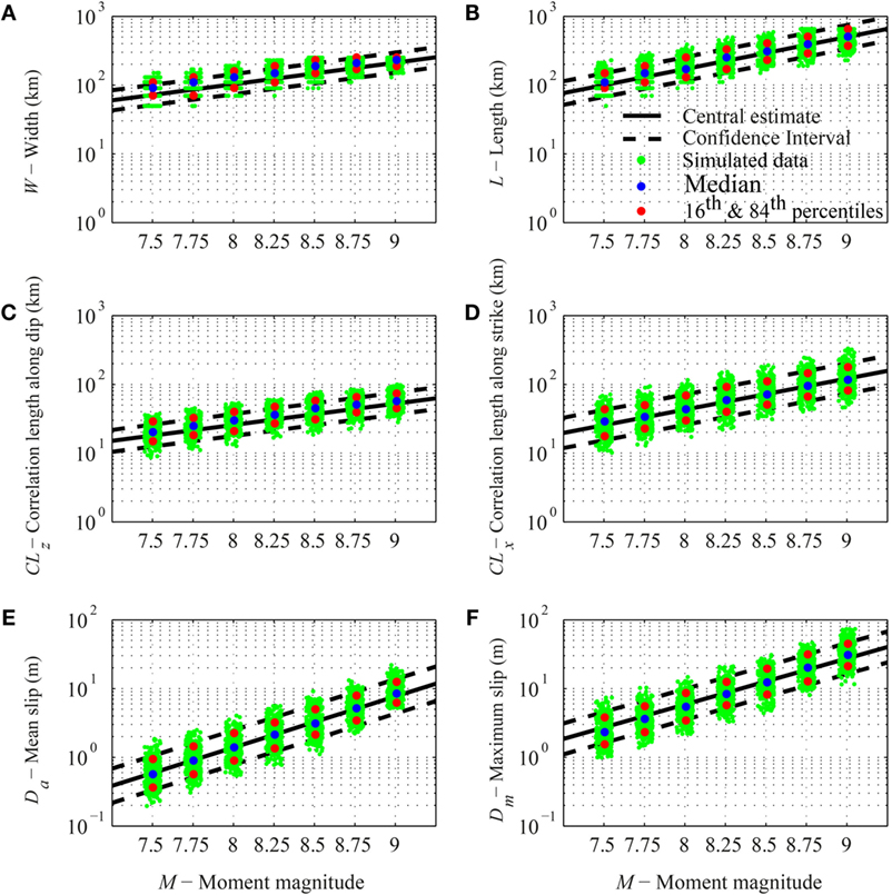
Figure 4. Scaling relationships for tsunamigenic earthquakes. (A) Rupture width versus moment magnitude. (B) Rupture length versus moment magnitude. (C) Correlation length along dip versus moment magnitude. (D) Correlation length along strike versus moment magnitude. (E) Mean slip versus moment magnitude. (F) Maximum slip versus moment magnitude. The simulated values (green dots) and the corresponding percentiles (colored circles) are also shown.

The preceding procedure of earthquake source characterization is innovative with respect to the literature. In particular, a common physical process for concurrent earthquake and tsunami threats is considered, i.e., the common fault rupture scenario that is modeled through the generic stochastic slip scenario on the subduction fault plane. The adoption of a common physical process facilitates the probabilistic investigation of the dependency between shaking and tsunami hazard parameters.

Earthquake Simulation

Ground motion prediction equations are extensively used as an effective way to predict seismic intensity measures for a given earthquake scenario (Wald et al., 2006). To account for seismic intensities at multiple locations that occur simultaneously for a given event, GMPEs together with spatial correlations in the regression residuals can be treated as statistical prediction models (Goda and Atkinson, 2010; Goda, 2011). This feature is particularly important in extending the seismic hazard assessment into a risk assessment of a portfolio of buildings/infrastructures. In this study, only the intra-event SD is propagated through the simulation procedure; such a choice is consistent with the simulation scenario of a single fault plane.

Two GMPEs that are applicable to subduction zones are used for the seismic simulations (Figure 2B). The first GMPE (Abrahamson et al., 2016) was developed with a global dataset of earthquakes in subduction zones and has been modified by adding the 2010 Maule Chile and 2011 Tohoku Japan earthquakes to the initial database. The basic functional form of the model for interface subduction events is

$\begin{array}{l}\ln \left(S_{\text{a}}\right)={\mathrm{\theta }}_1+{\mathrm{\theta }}_4\cdot \mathrm{\Delta }{C}_1+\left[{\mathrm{\theta }}_2+{\mathrm{\theta }}_3\cdot \left(M-7.8\right)\right]\cdot \ln \left\{R+C_4\cdot \exp \left[{\mathrm{\theta }}_9\cdot \left(M-6\right)\right]\right\}+{\mathrm{\theta }}_6\cdot R\hfill \\ +f_{\text{MAG}}\left(M\right)+f_{\text{FABA}}\left(R\right)+f_{\text{SITE}}\left(\text{PG}{\text{A}}_{1000},V_{\text{S}30}\right)+\mathrm{\sigma }\cdot \mathrm{\epsilon }\end{array}$ (13)

where ln is the natural logarithm, R is the closest distance to the rupture area, V_S30 is the shear wave velocity in the uppermost 30 m of soil column, PGA₁₀₀₀ is the median peak ground acceleration (PGA) value corresponding to V_S30 = 1000 m/s, σ is the total SD, and ε is the Gaussian error term, represented by 0 mean and unit SD. The SD is period-dependent; it is obtained by the combination of intra-event (ϕ) and inter-event (τ) SDs. The magnitude function is

$\begin{array}{l}\hfill f_{\text{MAG}}\left(M\right)=\left\{\begin{array}{cc}{\mathrm{\theta }}_4\cdot \left[M-\left(7.8+\mathrm{\Delta }{C}_1\right)\right]+{\mathrm{\theta }}_{13}\cdot {\left(10-M\right)}^2\hfill & \text{for}M\le 7.8+\mathrm{\Delta }{C}_1\hfill \\ {\mathrm{\theta }}_5\cdot \left[M-\left(7.8+\mathrm{\Delta }{C}_1\right)\right]+{\mathrm{\theta }}_{13}\cdot {\left(10-M\right)}^2\hfill & \text{for}M>7.8+\mathrm{\Delta }{C}_1\hfill \end{array}\right.\end{array}$ (14)

where ΔC₁ is the term representing the epistemic uncertainty in the break of the magnitude scaling and allows adjusting the GMPE for large interface events that were not originally considered in the earthquake database. f_FABA(R) represents the forearc/backarc scaling term; it is equal to 0 for forearc or unknown site, and this is applicable to the case of this study. Finally, the model for site response scaling is given by

$\begin{array}{ll}{f}_{\text{SITE}}=\hfill & {\mathrm{\theta }}_{12}\cdot \ln \left(\frac{\min \left(V_{S30},1000\right)}{V_{\text{lin}}}\right)-b\cdot \ln \left(\text{PG}{\text{A}}_{1000}+c\right)\hfill & \hfill \\ +b\cdot \ln \left[\text{PG}{\text{A}}_{1000}+c\cdot {\left(\frac{\min \left(V_{S30},1000\right)}{V_{\text{lin}}}\right)}^{\text{n}}\right]& V_{S30}<V_{\text{lin}}\\ f_{\text{SITE}}=\hfill \hfill & {\mathrm{\theta }}_{12}\cdot \ln \left(\frac{\min \left(V_{S30},1000\right)}{V_{\text{lin}}}\right)+b\cdot n\cdot \ln \left(\frac{\min \left(V_{S30},1000\right)}{V_{\text{lin}}}\right)\hfill & V_{S30}\ge V_{\text{lin}}\end{array}$ (15)

All the model coefficients for Eqs 13–15 can be found in Abrahamson et al. (2016).

The second GMPE by Morikawa and Fujiwara (2013) is suitable for M9 earthquakes in Japan. Two formulations are proposed: one is expressed with a quadratic magnitude term, while the other considers a linear magnitude term. In this study, the quadratic formulation is used since the correction factors (presented in the following) that are included in the quadratic formulation reduce the regression SD. The functional form for interface events is

$\begin{array}{l}\log \left(S_{\text{a}}\right)=a_1\cdot {\left(\min \left(M,8.2\right)-M\right)}^2+b_1\cdot R+c_1-\log \left(R+d_1\cdot {10}^{e_1\cdot \min \left(M,8.2\right)}\right)+\mathrm{\sigma }\cdot \mathrm{\epsilon }\hfill \end{array}$ (16)

where log is the base-10 logarithm, a₁, b₁, c₁, d₁, e₁, and σ are period-dependent regression coefficients and can be found in Morikawa and Fujiwara (2013). In Morikawa and Fujiwara (2013), no distinction is made between intra-event and inter-event SDs. The two SDs ϕ and τ can be determined by splitting the total variance into the intra-event and inter-event components based on the ratios of intra-event and inter-event variances to the total variance presented in Zhao et al. (2006). The estimate of the prediction equation is further modified using three additional correction terms: amplification due to the deep sedimentary layers (G_d), amplification due to shallow soft soils (G_s), and anomalous seismic intensity distribution due to the position of the site of interest with respect to the volcanic front (AI). In this study, only the second correction term is taken into account and is given by

$\log \left(G_{\text{s}}\right)=p_{\text{s}}\cdot \log \left[\frac{\min \left(V_{S_{\max }},V_{\text{S}30}\right)}{350}\right]$ (17)

where $V_{S_{\max }}$ is a period-dependent regression parameter that can be found in Morikawa and Fujiwara (2013).

Figures 5A–D compare the two GMPEs for three seismic intensity parameters [i.e., PGA, S_a(T = 0.3 s), and S_a(T = 3 s)], for M equal to 7.5 and 9.0 and for V_S30 equal to 300 m/s. Figure 6 shows the acceleration response spectra obtained using the two GMPEs, considering two values of closest distance (i.e., 50 and 200 km), and the same values of magnitude and V_S30 described before. Significant differences between the two GMPEs can be observed, especially for the large value of magnitude. Moreover, the Morikawa–Fuijwara GMPE tends to attenuate PGA and short-period spectral acceleration faster than the Abrahamson et al. GMPE with the distance, while the opposite trend occurs for the long-period spectral accelerations.

FIGURE 5

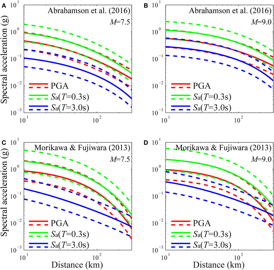
Figure 5. Comparison of GMPEs. (A) Abrahamson et al. GMPE for M = 7.5 and V_S30 = 300 m/s. (B) Abrahamson et al. GMPE for M = 9.0 and V_S30 = 300 m/s. (C) Morikawa–Fujiwara GMPE for M = 7.5 and V_S30 = 300 m/s. (D) Morikawa–Fujiwara GMPE for M = 9.0 and V_S30 = 300 m/s.

FIGURE 6

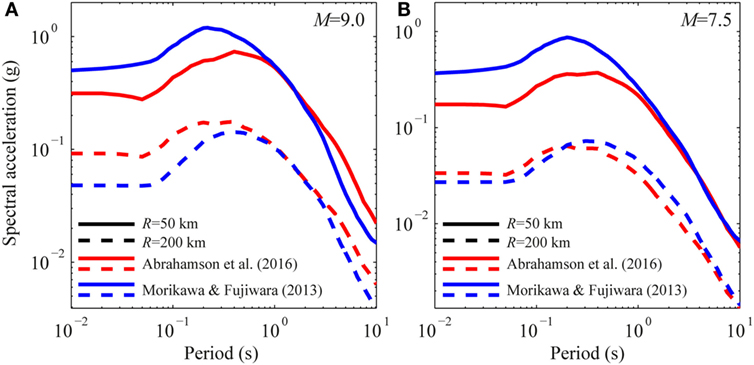
Figure 6. Response spectra obtained considering the Abrahamson et al. and Morikawa–Fujiwara GMPEs, V_S30 = 300 m/s, and two shortest distances (R = 50 and 200 km). (A) M = 7.5. (B) M = 9.0.

For seismic simulations, three main inputs are required: event magnitude, distance from the rupture, and shear wave velocity for the considered site. Regarding the distance from the rupture, the GMPEs presented above are both based on the closest distance between the location of interest and the rupture area (Figure 7A). To optimize the computation of the shortest distance, the distances between the coastline location and each discretized element of the 2011 Tohoku-type fault are precomputed and stored (Figure 7B). As an example, Figure 7C shows the distances computed for 500 stochastic scenarios, which are considered in Section “Results.” It is worth noting that the minimum distance is circa 50 km, corresponding to the depth of the fault plane under the considered location. As observed in Goda and Atkinson (2014), the source-to-site distance is affected by the location and size of the fault plane, which in turn is determined by the magnitude of the event. In Figure 7C, it can be observed that the greater magnitude value results in smaller variability of the closest distance (i.e., distribution function has a steeper slope). This is because the rupture plane can move more freely within the overall fault plane (Figure 2A) when the earthquake magnitude is small. For the shear wave velocity, the USGS global V_S30 map server is used (Wald and Allen, 2007).

FIGURE 7

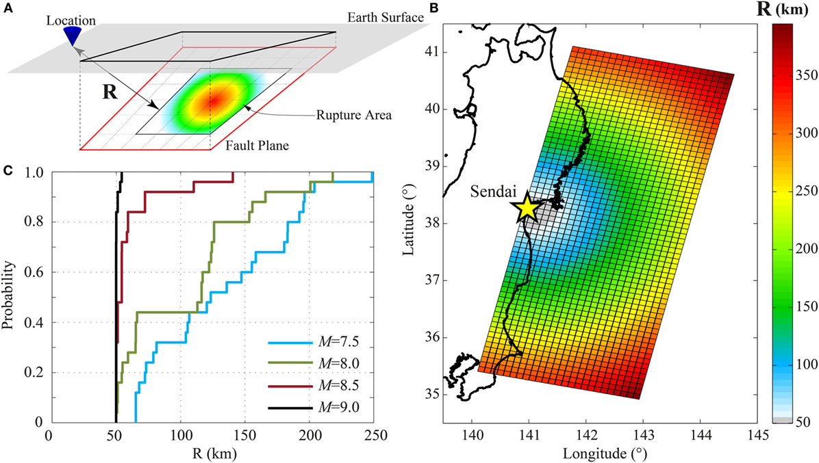
Figure 7. (A) Schematic representation of the shortest distance from the rupture. (B) Precalculated distance for each sub-fault from a site in Sendai City. (C) Distribution of the distances for 500 stochastic simulations associated with 4 values of magnitude.

Finally, to generate shake maps of intensity measures IM, the multivariate lognormal distribution can be adopted. The median values of IM at sites of interest are calculated from the GMPE, whereas their variances are based on the intra-event components. The prediction errors ε in the GMPE are spatially correlated; the correlation coefficient matrix has diagonal elements equal to 1 and off-diagonal elements equal to the correlation coefficient ρ. The correlation coefficient can be calculated using the following equation (Goda and Atkinson, 2010):

${\mathrm{\rho }}_{\text{i,j}}\left(\mathrm{\Delta }\right)=\max \left[\mathrm{\gamma }\cdot \exp \left(-\mathrm{\alpha }\cdot {\mathrm{\Delta }}^{\mathrm{\beta }}\right)-\mathrm{\gamma }+1,0\right]$ (18)

where Δ is the distance between the points i and j, while α, β, and γ are period-dependent model parameters that can be found in Goda and Atkinson (2010).

Tsunami Simulation

For each stochastic event, a tsunami simulation is carried out in order to compute the maximum inundation intensity measure (Figure 2C). To optimize the computational time, the subduction plane is discretized into sub-faults of 10 km × 10 km (Figure 3A), and for each sub-fault, the seafloor displacement corresponding to 1 m of slip is calculated using analytical equations by Okada (1985) and Tanioka and Satake (1996). Subsequently, for each simulated earthquake slip (i.e., event), the overall seafloor displacement field is estimated by scaling and summing the seafloor deformation fields of all individual sub-faults that make up the event.

Tsunami modeling is then carried out using a well-tested numerical code of Goto et al. (1997) that is capable of generating offshore tsunami propagation and inundation profiles by evaluating non-linear shallow water equations, with run-up using a leapfrog staggered-grid finite difference scheme. The run-up calculation is based on a moving boundary approach, where a dry/wet condition of a computational cell is determined based on total water depth relative to its elevation. The numerical tsunami calculation is performed for duration sufficient to model the most critical phases of tsunami waves (i.e., 2 h). The integration time step is determined by satisfying the CFL condition; it depends on the bathymetry/elevation data, and their grid sizes and is typically between 0.1 and 0.5 s. For the simulation, it is possible to obtain the maximum tsunami intensity measures of interest (i.e., tsunami height, tsunami velocity, etc.) for one or more specific locations along the coast. The results can also be used to evaluate aggregate tsunami hazard parameters, such as inundation areas above a certain depth.

A complete dataset of bathymetry/elevation, coastal/riverside structures (e.g., breakwater and levees), and surface roughness is obtained from the Miyagi prefectural government. The data are provided in the form of nested grids (1350 m–450 m–150 m– 50 m), covering the geographical regions of Tohoku. The ocean-floor topography data are based on the 1:50,000 bathymetric charts and JTOPO30 database developed by Japan Hydrographic Association and based on the nautical charts developed by Japan Coastal Guard. The tidal fluctuation is not taken into account in this study. The elevation data of the coastal/riverside structures are primarily provided by municipalities. In the tsunami simulation, the coastal/riverside structures are represented by a vertical wall at one or two sides of the computational cells. To evaluate the volume of water that overpasses these walls, Homma’s overflowing formulae are employed. In the tsunami simulation, the bottom friction is evaluated using the Manning’s formula. The Manning’s coefficients are assigned to computational cells based on national land use data in Japan: 0.02 m^−1/3s for agricultural land, 0.025 m^−1/3s for ocean/water, 0.03 m^−1/3s for forest vegetation, 0.04 m^−1/3s for low-density residential areas, 0.06 m^−1/3s for moderate-density residential areas, and 0.08 m^−1/3s for high-density residential areas.

Development of Earthquake–Tsunami Hazard Curves

For each value of magnitude, the simulations are used to evaluate the term P(IM ≥ im|M) for the location of interest. Such probability is represented by the CCDF of the IM (Figure 2D). Specifically, the CCDF of the IM (i.e., spectral acceleration or tsunami inundation) is obtained as the Kaplan–Meier estimator (Kaplan and Meier, 1958), for which the variance can be calculated through the Greenwood’s formula (Greenwood, 1926), and therefore, a confidence interval around the central estimate can be obtained. In this study, the 95% confidence interval is considered.

The curves obtained in the previous step for each magnitude are then multiplied by the probabilities corresponding to the related magnitude and eventually are summed up (Figure 2E). Also in this case, three curves are obtained, one corresponding to the central value and two for the confidence interval. The final hazard curves, representing the mean annual rate of occurrence of specific values of earthquake–tsunami intensity measures, are obtained by multiplying the previous three conditional curves (for each hazard) by the occurrence rate of events with magnitudes greater than the minimum magnitude considered in the magnitude–frequency distribution.

Results

The developed methodology is applied to calculate the earthquake and tsunami hazard curves for a site along the coast line of Sendai City, Miyagi Prefecture (the yellow star in Figure 7B), for which V_S30 = 240 m/s is obtained based on the USGS data. It is interesting to note that during the 2011 Tohoku earthquake, PGA of 0.8 g (Wald et al., 2006; USGS ShakeMap Archive, 2016) and tsunami wave height of 7 m [Ministry of Land, Infrastructure, and Transportation (MLIT), 2014] were observed in the vicinity of this site. The main results that are discussed in this section focus on (a) sensitivity of seismic and tsunami hazard estimates to the number of stochastic simulations, and (b) development of earthquake–tsunami multi-hazard curves for the target site and the deaggregation of the seismic and tsunami hazards. The former provides useful information regarding the stability of the simulation-based hazard assessments.

Sensitivity of Seismic and Tsunami Hazard Parameters to the Number of Simulations

Short or incomplete records lead to biased estimation of the hazard parameters, especially when conventional statistical methods are used (Lamarre et al., 1992). To investigate the effect of the number of simulations on the final hazard estimation, a bootstrap procedure is carried out by randomly sampling m values from the original sample containing n elements (with m ≤ n). This provides a pool of different samples of independent and identically distributed random variables, whose distribution function is the same as that of the original sample. For each generated sample, statistics of the parameter of interest (e.g., mean, median, and different percentiles) are then computed. The ensemble of such estimates can be used to quantify the uncertainty in the parameter value.

Figures 8 and 9 show five percentiles (i.e., 5th, 25th, 50th, 75th, and 95th) of the spectral acceleration and wave height, respectively; such intensity measures are calculated for the site in Sendai by considering different magnitude values (i.e., 7.5, 8.0, 8.5, and 9.0) as a function of the number of simulations. Moreover, Figure 8 shows bootstrap results for the seismic case considering two different GMPEs. The analysis is carried out for the maximum sample size of n = 500 simulations. The bootstrap procedure is then applied considering the number of simulations m varying between 1 and 500. For each trial number of simulations m, 1000 Monte Carlo samples are generated, and then the percentile curves are obtained as the mean value of such simulations. Based on Figure 8, it can be concluded that for the considered seismic case, 200 simulations is sufficient to observe stable percentiles for all magnitude values and for both GMPEs considered. Also in this case, for increasing values of magnitude, there is a decreasing trend of variability of the simulated values due to the reduction in variability of the closest distance (Figure 7C).

FIGURE 8

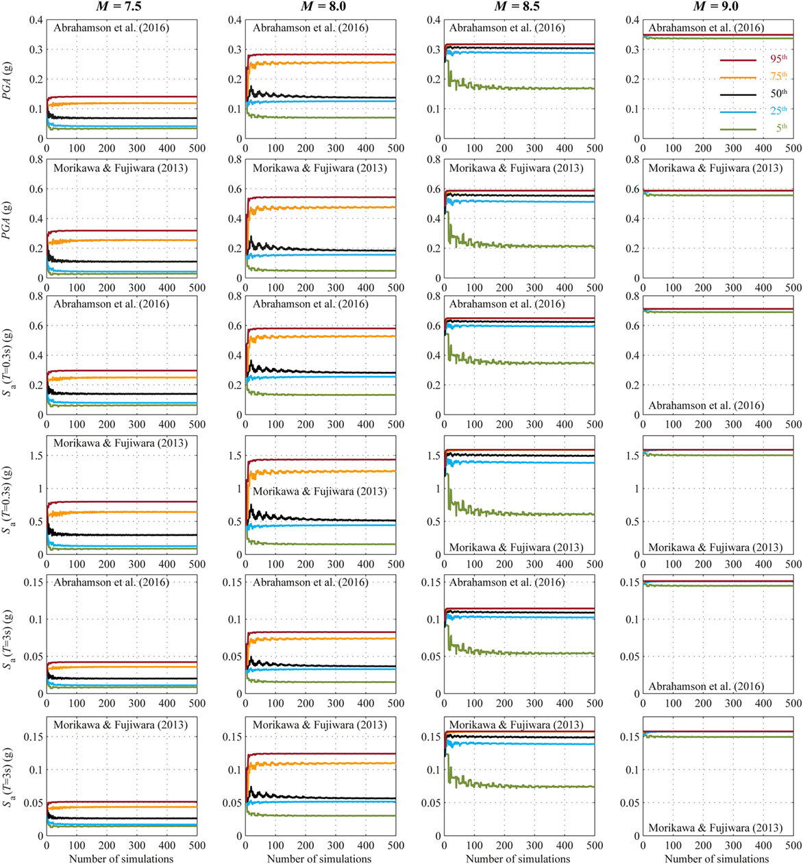
Figure 8. Convergence of estimated seismic intensity measures [i.e., PGA, S_a(T = 0.3 s) and S_a(T = 3 s)] as a function of the number of simulations by considering the Abrahamson et al. and Morikawa–Fujiwara GMPEs and four moment magnitudes (M = 7.5, 8.0, 8.5, and 9.0). Different colors represent different percentiles.

FIGURE 9

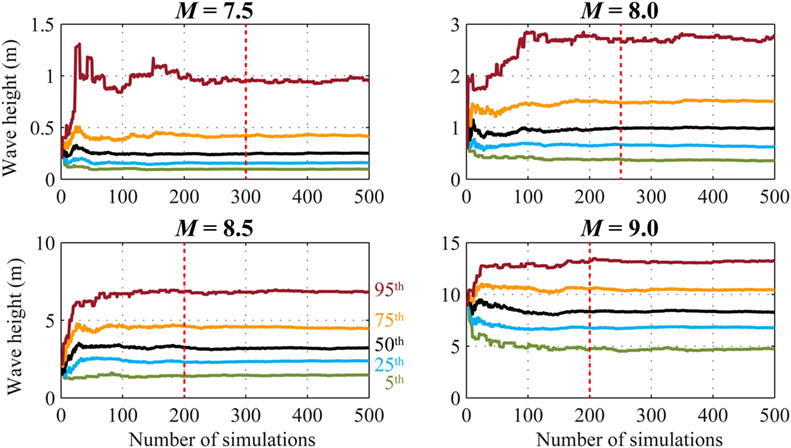
Figure 9. Convergence of estimated tsunami intensity measures (wave height) as a function of the number of simulations by considering four moment magnitudes (M = 7.5, 8.0, 8.5, and 9.0).

Tsunami simulation results show that the 50th percentile curves are stable after 100 simulations for all the considered magnitude values. To obtain stable estimates of the high percentiles, a larger number of simulations are needed (the red dotted line in Figure 9). In particular, 300 simulations are necessary for M7.5, 250 simulations for M8.0, and 200 simulations for M8.5 and M9.0. Such a decreasing trend with the magnitude is consistent with what was observed for the rupture distance (Figure 7C), i.e., when the magnitude is relatively small, the variability of the inundation intensity measures are increased because the rupture area can move more freely within the fault plane. In turn, when the magnitude is large, the fluctuation of the rupture area is more constrained.

Considering the results shown in Figures 8 and 9, 300 stochastic simulations are carried out for the final coupled multi-hazard simulation process in the following. The calculation can be completed in less than 1 week using a conventional workstation with parallel processing.

Earthquake–Tsunami Hazard Curves

For each value of 7 magnitudes (i.e., 7.5, 7.75, 8.0, 8.25, 8.5, 8.75, and 9.0), 300 sets of the source parameters θ are generated using the scaling relationships by Goda et al. (2016). Figure 4 shows the simulated source parameters (the green dots). Simulated data are in agreement with the source parameter distributions (i.e., green dots are well clustered within the confidence interval of the scaling relationships). Then, 300 simulations are carried out for the earthquake hazard and tsunami hazard analysis, starting from the same stochastic source models.

The CCDFs (Figure 2D) in terms of PGA, S_a(T = 0.3 s), and S_a(T = 3 s) are shown in Figures 10A,C,E, respectively, for all the magnitude values analyzed. The analogous CCDFs for the tsunami wave height are presented in Figure 11A. Figures 10B,D,F and 11B show the CCDFs, weighted by the probability values obtained from the discretized Gutenberg–Richter relationship (Figure 3D).

FIGURE 10

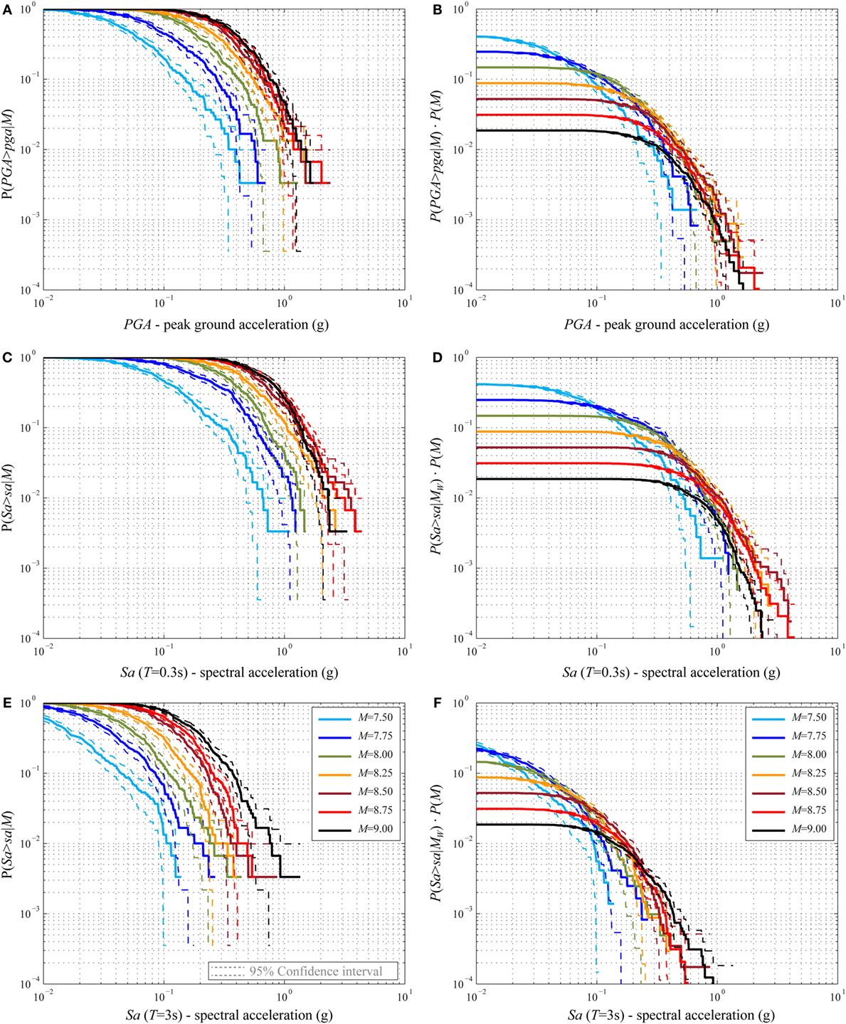
Figure 10. (A) Conditional hazard curve for PGA. (B) Weighted conditional hazard curves for PGA. (C) Conditional hazard curve for S_a(T = 0.3 s). (D) Weighted conditional hazard curves for S_a(T = 0.3 s). (E) Conditional hazard curve for S_a(T = 3 s). (F) Weighted conditional hazard curves for S_a(T = 3 s).

FIGURE 11

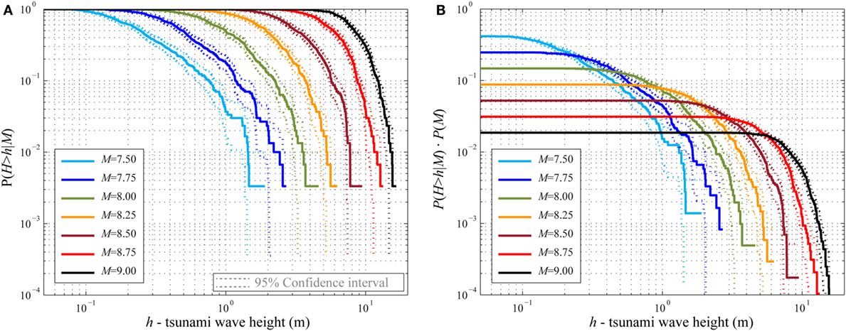
Figure 11. (A) Conditional hazard curve for tsunami wave height. (B) Weighted conditional hazard curves for tsunami wave height.

As shown in Figure 2E, for each IM [i.e., PGA, S_a(T), h, etc.], the summation of the curves presented in Figures 10B,D,F and 11B, multiplied by λ(M ≥ 7.375) = 0.183, leads to the final hazard curves. Figures 12A–C shows the final hazard curves, and the 95% confidence interval, for PGA, S_a(T = 0.3 s), and S_a(T = 3 s) obtained using the two GMPEs, i.e., Abrahamson et al. (2016), represented with blue lines, and Morikawa and Fujiwara (2013), represented with red lines. In the same figures, the mean seismic hazard curves are represented with black lines. Similarly, Figure 12D shows the final tsunami hazard curve and its 95% confidence interval that is very tight around the central estimate curve. It is noteworthy that the steep slope of the final tsunami hazard curve for wave heights greater than 10 m is because the tsunami height cannot be so high in the Sendai plain areas unlike ria-type coastal areas (e.g., Onagawa and Kesennuma), where the wave amplification due to topographical effects is significant.

FIGURE 12

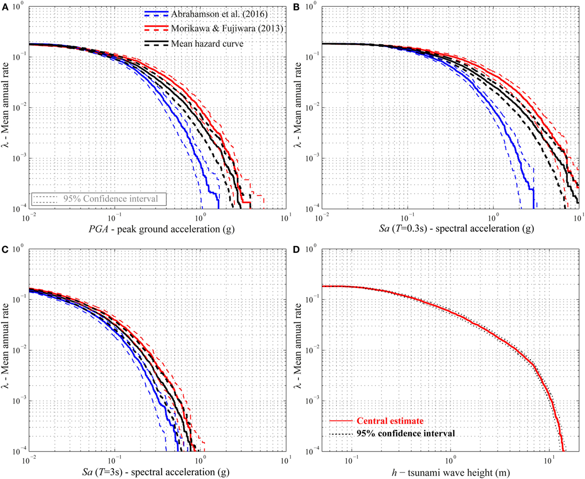
Figure 12. (A) Final seismic hazard curves for PGA. (B) Final seismic hazard curves for S_a(T = 0.3 s). (C) Final seismic hazard curves for S_a(T = 3 s). (D) Final tsunami hazard curves.

Seismic Uniform Hazard Spectra and Earthquake–Tsunami Deaggregation

The proposed procedure also facilitates the construction of uniform hazard spectra (UHS) for seismic hazard. By repeating the seismic simulations for several spectral accelerations (Figure 13A) and considering specific values of the mean annual rate (e.g., 2, 5, and 10% in 50 years), it is possible to obtain the UHS, as shown in Figure 13B. The hazard curves and spectra are jagged because of the limited number of simulations (i.e., 300). Since the seismic simulations are less time consuming with respect to the tsunami simulations, it is possible to increase the number of simulations; in particular, for each scenario, several thousands of simulations can be conducted with a low additional computational effort. Figure 13C shows the seismic hazard curves obtained by performing 300 × 5000 simulations (i.e., 5000 simulations for each stochastic simulation). By increasing the number of simulations, the UHS become smooth (Figure 13D), and the confidence intervals around the central estimate hazard curves become narrow.

FIGURE 13

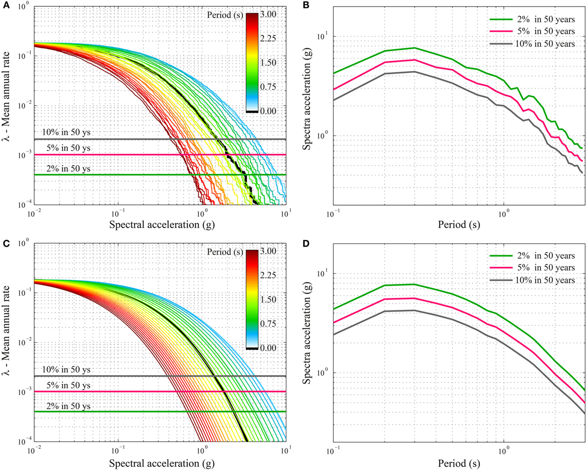
Figure 13. (A) Final seismic hazard curves for intensity parameters from PGA (the black line) to S_a(T = 3 s) based on 300 simulations. (B) Uniform hazard spectra based on 300 simulations. (C) Final seismic hazard curves for intensity parameters from PGA (the black line) to S_a(T = 3 s) based on 300 × 5000 simulations. (D) Uniform hazard spectra based on 300 × 5000 simulations.

As a byproduct of the procedure, the earthquake–tsunami hazard deaggregation is obtained. Deaggregation shows the relative contributions of dominant seismic scenarios to the specified hazard levels and can be represented in terms of distance and magnitude. The deaggregation of the two hazards for the same mean annual rate of occurrence is demonstrated. Figure 14 shows the deaggregation results for Sendai by considering PGA (Figures 14A,C) and tsunami inundation height (Figures 14B,D) corresponding to two values of mean annual rate of occurrence (i.e., 63 and 10% in 50 years). The 10% in 50-year hazard level (corresponding to an event with 475-year return period) is commonly used to describe the life safety limit state, whereas the 63% in 50-year hazard level (corresponding to an event with 50-year return period) corresponds to the damage control limit state (CEN, 2004). It is worth noting that only large magnitude events contribute to higher values of IMs. Moreover, as observed before, the larger the magnitude is, the less the distance is influential. Finally, it is interesting to observe that the combinations of magnitude and distance that affect the seismic hazard and tsunami hazard differ significantly.

FIGURE 14

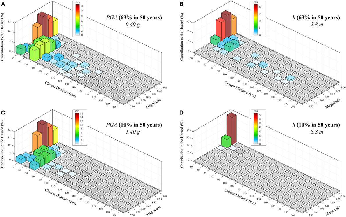
Figure 14. (A) Seismic hazard deaggregation for PGA corresponding to the hazard level of 63% in 50 years. (B) Tsunami hazard deaggregation for wave height corresponding to the hazard level of 63% in 50 years. (C) Seismic hazard deaggregation for PGA corresponding to the hazard level of 10% in 50 years. (D) Tsunami hazard deaggregation for wave height corresponding to the hazard level of 10% in 50 years.

Conclusion

A new simulation-based procedure to probabilistically calculate the earthquake–tsunami multi-hazard for specific locations was presented. The simulation framework allows implementing all potential sources of uncertainties, both epistemic and aleatory. The slip distribution on the fault plane was characterized in detail since it represents the major source of uncertainty. To generate a wide range of earthquake scenarios, new global scaling relationships of earthquake source parameters for tsunamigenic events were used. For each discrete magnitude value, multiple realizations of possible earthquake slip distributions were generated. The procedure was applied to the Tohoku region (Japan), and a single point located on the coastline in Sendai City was considered for assessing the concurrent earthquake–tsunami hazard. Three hundred simulations were performed for both seismic and tsunami intensity estimations at each discrete magnitude value. Data obtained from simulations were used to calculate the CCDFs of the considered intensity measures (i.e., spectral acceleration and tsunami inundation height) and their confidence intervals. Finally, such curves were combined with the magnitude–frequency distribution and were summed up in order to obtain the final triplets of earthquake–tsunami hazard curves: one representative of the central estimate and the others corresponding to the 95% confidence interval.

Based on the analysis results, the following conclusions can be drawn:

(a) For the considered case study, 300 simulations were sufficient to obtain a reliable and stable representation of both earthquake and tsunami hazard parameters at a single location, both in terms of central estimates and high percentiles.

(b) Given the same number of simulations and passing from small magnitude to large magnitude, a decrease in the dispersion of the simulation results was observed. This is due to the decreased variability of the earthquake location on the fault, and it also implies a reduction of the confidence interval.

(c) The procedure facilitates the calculation of UHS for seismic hazard and the deaggregation of both seismic and tsunami hazards.

The presented work can be considered a first step toward an earthquake–tsunami multi-hazard performance-based framework; in fact, a multi-risk assessment can be carried out by convoluting the obtained multi-hazard curves with seismic and tsunami fragility curves. The work can be extended using a Bayesian robust methodology (Cheung and Beck, 2010) to make more reliable estimations of earthquake–tsunami hazards. The proposed method can be further integrated into an operational tool for real-time earthquake–tsunami forecast (Tsushima et al., 2011) using data from offshore buoy and ocean-bottom pressure gauges. Furthermore, the methodology can be expanded to obtain the conditional tsunami or seismic hazard curve, given that a specific value of the counterpart hazard has been selected.

Author Contributions

The two co-authors contributed equally to this work.

Conflict of Interest Statement

The authors declare that the research was conducted in the absence of any commercial or financial relationships that could be construed as a potential conflict of interest.

Acknowledgments

This work is funded by the Engineering and Physical Sciences Research Council (EP/M001067/1).

References

Abrahamson, N., Gregor, N., and Addo, K. (2016). BC hydro ground motion prediction equations for subduction earthquakes. Earthquake Spectra 32, 23–44. doi: 10.1193/051712EQS188MR

CrossRef Full Text | Google Scholar

Akkar, S., and Cheng, Y. (2015). Application of a Monte-Carlo simulation approach for the probabilistic assessment of seismic hazard for geographically distributed portfolio. Earthquake Eng. Struct. Dyn. 45, 525–541. doi:10.1002/eqe.2667

CrossRef Full Text | Google Scholar

Annaka, T., Satake, K., Sakakiyama, T., Yanagisawa, K., and Shuto, N. (2007). Logic-tree approach for probabilistic tsunami hazard analysis and its applications to the Japanese coasts. Pure Appl. Geophys. 164, 577–592. doi:10.1007/s00024-006-0174-3

CrossRef Full Text | Google Scholar

Atkinson, G. M., and Goda, K. (2013). “Probabilistic seismic hazard analysis of civil infrastructure: chapter 1, 3–28,” in Handbook of Seismic Risk Analysis and Management of Civil Infrastructure Systems, eds S. Tesfamariam and K. Goda (Cambridge: Woodhead Publishing), 912.

Google Scholar

Billi, A., Funiciello, R., Minelli, L., Faccenna, C., Neri, G., Orecchio, B., et al. (2008). On the cause of the 1908 Messina tsunami, southern Italy. Geophys. Res. Lett. 35, L06301. doi:10.1029/2008GL033251

CrossRef Full Text | Google Scholar

Box, G. E. P., and Cox, D. R. (1964). An analysis of transformations. J. R. Stat. Soc. Ser. B 26, 211–252.

Google Scholar

Burbidge, D., Cummins, P. R., Mleczko, R., and Thio, H. K. (2008). A probabilistic tsunami hazard assessment for Western Australia. Pure Appl. Geophys. 165, 2059–2088. doi:10.1007/s00024-008-0421-x

CrossRef Full Text | Google Scholar

Burroughs, S. M., and Tebbens, S. F. (2005). Power-law scaling and probabilistic forecasting of tsunami runup heights. Pure Appl. Geophys. 162, 331–342. doi:10.1007/s00024-004-2603-5

CrossRef Full Text | Google Scholar

CEN. (2004). Eurocode 8: Design of Structures for Earthquake Resistance – Part 1: General Rules, Seismic Actions and Rules for Buildings. Brussels: Comite International de Normalization.

Google Scholar

Cheung, K. F., Wei, Y., Yamazaki, Y., and Yim, S. C. (2011). Modeling of 500-year tsunamis for probabilistic design of coastal infrastructure in the Pacific Northwest. Coast. Eng. J. 58, 970–985. doi:10.1016/j.coastaleng.2011.05.003

CrossRef Full Text | Google Scholar

Cheung, S. H., and Beck, J. L. (2010). Calculation of posterior probabilities for Bayesian model class assessment and averaging from posterior samples based on dynamic system data. Comput. Aided Civil Infrastruct. Eng. 25, 304–321. doi:10.1111/j.1467-8667.2009.00642.x

CrossRef Full Text | Google Scholar

Cornell, C. A. (1968). Engineering seismic risk analysis. Bull. Seismol. Soc. Am. 58, 1583–1606.

Google Scholar

Downes, G. L., and Stirling, M. W. (2001). “Groundwork for development of a probabilistic tsunami hazard model for New Zealand,” in Proceedings of International Tsunami Symposium, Session 1 (Seattle, USA: National Oceanic and Atmospheric Administration), 293–301.

Google Scholar

Farreras, S., Ortiz, M., and Gonzalez, J. I. (2007). Steps towards the implementation of a tsunami detection, warning, mitigation and preparedness program for southwestern coastal areas of Mexico. Pure Appl. Geophys. 164, 605–616. doi:10.1007/s00024-006-0175-2

CrossRef Full Text | Google Scholar

Fukutani, Y., Suppasri, A., and Imamura, F. (2016). Stochastic analysis and uncertainty assessment of tsunami wave height using a random source parameter model that targets a Tohoku-type earthquake fault. Stoch. Environ. Res. Risk Assess. 29, 1763–1779. doi:10.1007/s00477-014-0966-4

CrossRef Full Text | Google Scholar

Geist, E. L. (2002). Complex earthquake rupture and local tsunamis. J. Geophys. Res. Solid Earth 107, ESE 2-1–ESE 2-15. doi:10.1029/2000JB000139

CrossRef Full Text | Google Scholar

Geist, E. L. (2005). Local Tsunami Hazards in the Pacific Northwest from Cascadia Subduction Zone Earthquakes. Reston: U.S. Geological Survey, 17. Professional Paper 1661-B.

Google Scholar

Geist, E. L., and Dmowska, R. (1999). Local tsunamis and distributed slip at the source. Pure Appl. Geophys. 154, 485–512. doi:10.1007/s000240050241

CrossRef Full Text | Google Scholar

Geist, E. L., and Parsons, T. (2006). Probabilistic analysis of tsunami hazards. Nat. Hazards 37, 277–314. doi:10.1007/s11069-005-4646-z

CrossRef Full Text | Google Scholar

Goda, K. (2011). Interevent variability of spatial correlation of peak ground motions and response spectra. Bull. Seismol. Soc. Am. 101, 2522–2531. doi:10.1785/0120110092

CrossRef Full Text | Google Scholar

Goda, K., and Atkinson, G. M. (2010). Intraevent spatial correlation of ground-motion parameters using SK-net data. Bull. Seismol. Soc. Am. 100, 3055–3067. doi:10.1785/0120100031

CrossRef Full Text | Google Scholar

Goda, K., and Atkinson, G. M. (2014). Variation of source-to-site distance for megathrust subduction earthquakes: effects on ground motion prediction equations. Earthquake Spectra 30, 845–866. doi:10.1193/080512EQS254M

CrossRef Full Text | Google Scholar

Goda, K., Mai, P. M., Yasuda, T., and Mori, N. (2014). Sensitivity of tsunami wave profiles and inundation simulations to earthquake slip and fault geometry for the 2011 Tohoku earthquake. Earth Planets Space 66:105. doi:10.1186/1880-5981-66-105

CrossRef Full Text | Google Scholar

Goda, K., Yasuda, T., Mori, N., and Maruyama, T. (2016). New scaling relationships of earthquake source parameters for stochastic tsunami simulation. Coast. Eng. J. 58:1650010. doi:10.1142/S0578563416500108

CrossRef Full Text | Google Scholar

González, F. I., Geist, E. L., Jaffe, B., Kânoglu, U., Mofjeld, H., Synolakis, C. E., et al. (2009). Probabilistic tsunami hazard assessment at Seaside, Oregon, for near- and far-field seismic sources. J. Geophys. Res. Oceans 114, C11023. doi:10.1029/2008JC005132

CrossRef Full Text | Google Scholar

Goto, C., Ogawa, Y., Shuto, N., and Imamura, F. (1997). Numerical Method of Tsunami Simulation with the Leap-Frog Scheme (IUGG/IOC Time Project), IOC Manual. Paris, France: UNESCO.

Google Scholar

Greenwood, M. (1926). The Natural Duration of Cancer. Reports on Public Health and Medical Subjects, Vol. 33. London: Her Majesty’s Stationery Office, 1–26.

Google Scholar

Grezio, A., Gasparini, P., Marzocchi, W., Patera, A., and Tinti, S. (2012). Tsunami risk assessments in Messina, Sicily – Italy. Nat. Hazards Earth Syst. Sci. 12, 151–163. doi:10.5194/nhess-12-151-2012

CrossRef Full Text | Google Scholar

Grezio, A., Marzocchi, W., Sandri, L., and Gasparini, P. (2010). A Bayesian procedure for probabilistic tsunami hazard assessment. Nat. Hazards 53, 159–174. doi:10.1007/s11069-009-9418-8

CrossRef Full Text | Google Scholar

Guidoboni, E., and Comastri, A. (1997). The large earthquake of 8 August 1303 in Crete: seismic scenario and tsunami in the Mediterranean area. J. Seismol. 1, 55–72. doi:10.1023/A:1009737632542

CrossRef Full Text | Google Scholar

Gutenberg, B., and Richter, C. F. (1956). Magnitude and energy of earthquakes. Ann. Geophys. 9, 1–15.

Google Scholar

Headquarters for Earthquake Research Promotion. (2013). Investigations of Future Seismic Hazard Assessment. Tokyo: Japanese Govern, 217.

Google Scholar

Horspool, N., Pranantyo, I., Griffin, J., Latief, H., Natawidjaja, D. H., Kongko, W., et al. (2014). A probabilistic tsunami hazard assessment for Indonesia. Nat. Hazards Earth Syst. Sci. 14, 3105–3122. doi:10.5194/nhess-14-3105-2014

CrossRef Full Text | Google Scholar

Kaplan, E. L., and Meier, P. (1958). Nonparametric estimation from incomplete observations. J. Am. Stat. Assoc. 53, 457–481. doi:10.1080/01621459.1958.10501452

CrossRef Full Text | Google Scholar

Lamarre, M., Townshend, B., and Shah, H. C. (1992). Application of the bootstrap method to quantify uncertainty in seismic hazard estimates. Bull. Seismol. Soc. Am. 82, 104–119.

Google Scholar

Latter, J. H. (1981). Tsunamis of volcanic origin: summary of causes, with particular reference to Krakatoa, 1883. Bull. Volcanol. 44, 467–490. doi:10.1007/BF02600578

CrossRef Full Text | Google Scholar

Lavallée, D., Liu, P., and Archuleta, R. J. (2006). Stochastic model of heterogeneity in earthquake slip spatial distributions. Geophys. J. Int. 165, 622–640. doi:10.1111/j.1365-246X.2006.02943.x

CrossRef Full Text | Google Scholar

Liu, Y., Santos, A., Wang, S. M., Shi, Y., Liu, H., and Yuen, D. A. (2007). Tsunami hazards along Chinese coast from potential earthquakes in South China Sea. Phys. Earth Planet. Inter. 163, 233–244. doi:10.1016/j.pepi.2007.02.012

CrossRef Full Text | Google Scholar

Løvholt, F., Glimsdal, S., Harbitz, C. B., Horspool, N., Smebye, H., de Bono, A., et al. (2014). Global tsunami hazard and exposure due to large co-seismic slip. Int. J. Disaster Risk Reduct. 10, 406–418. doi:10.1016/j.ijdrr.2014.04.003

CrossRef Full Text | Google Scholar

Løvholt, F., Glimsdal, S., Harbitz, C. B., Zamora, N., Nadim, F., Peduzzi, P., et al. (2012). Tsunami hazard and exposure on the global scale. Earth-Sci. Rev. 110, 58–73. doi:10.1016/j.earscirev.2011.10.002

CrossRef Full Text | Google Scholar

Mai, P. M., and Beroza, G. C. (2002). A spatial random field model to characterize complexity in earthquake slip. J. Geophys. Res. Solid Earth 107, ESE 10-1–ESE 10-21. doi:10.1029/2001JB000588

CrossRef Full Text | Google Scholar

Mai, P. M., and Thingbaijam, K. K. S. (2014). SRCMOD: an online database of finite-fault rupture models. Seismol. Res. Lett. 85, 1348–1357. doi:10.1785/0220140077

CrossRef Full Text | Google Scholar

Matthews, M. V., Ellsworth, W. L., and Reasenberg, P. A. (2002). A Brownian model for recurrent earthquakes. Bull. Seismol. Soc. Am. 92, 2233–2250. doi:10.1785/0120010267

CrossRef Full Text | Google Scholar

McGuire, R. K. (2008). Probabilistic seismic hazard analysis: early history. Earthquake Eng. Struct. Dyn. 37, 329–338. doi:10.1002/eqe.765

CrossRef Full Text | Google Scholar

Ministry of Land, Infrastructure, and Transportation (MLIT). (2014). Survey of Tsunami Damage Condition. Available at: http://www.mlit.go.jp/toshi/toshi-hukkou-arkaibu.html

Google Scholar

Mofjeld, H. O., González, F. I., Titov, V. V., Venturato, A. J., and Newman, J. C. (2007). Effects of tides on maximum tsunami wave heights: probability distributions. J. Atmos. Oceanic Technol. 24, 117–123. doi:10.1175/JTECH1955.1

CrossRef Full Text | Google Scholar

Monastersky, R. (2012). The next wave. Nature 483, 144–146. doi:10.1038/483144a

CrossRef Full Text | Google Scholar

Morikawa, N., and Fujiwara, H. (2013). A new ground motion prediction equation for Japan applicable up to M9 mega-earthquake. J. Disaster Res. 8, 878–888. doi:10.20965/jdr.2013.p0878

CrossRef Full Text | Google Scholar

NGDC. (2016). National Geophysical Data Center (NGDC WDS) Global Historical Tsunami Database. Boulder, CO, USA. Available at: https://www.ngdc.noaa.gov/hazard/tsu_db.shtml

Google Scholar

Okada, Y. (1985). Surface deformation due to shear and tensile faults in a half-space. Bull. Seismol. Soc. Am. 75, 1135–1154.

Google Scholar

Orfanogiannaki, K., and Papadopoulos, G. A. (2007). Conditional probability approach of the assessment of tsunami potential: application in three tsunamigenic regions of the Pacific Ocean. Pure Appl. Geophys. 164, 593–603. doi:10.1007/s00024-006-0170-7

CrossRef Full Text | Google Scholar

Pardo-Iguzquiza, E., and Chica-Olmo, M. (1993). The Fourier integral method: an efficient spectral method for simulation of random fields. Math. Geol. 25, 177–217. doi:10.1007/BF00893272

CrossRef Full Text | Google Scholar

Parsons, T., and Geist, E. L. (2008). Tsunami probability in the Caribbean region. Pure Appl. Geophys. 165, 2089–2116. doi:10.1007/s00024-008-0416-7

CrossRef Full Text | Google Scholar

Power, W., Downes, G., and Stirling, M. (2007). Estimation of tsunami hazard in New Zealand due to South American earthquakes. Pure Appl. Geophys. 164, 547–564. doi:10.1007/s00024-006-0166-3

CrossRef Full Text | Google Scholar

Satake, K. (2001). “Tsunami modeling from submarine landslides,” in Proceedings of the International Tsunami Symposium, Session 6 (Seattle, USA: National Oceanic and Atmospheric Administration), 665–674.

Google Scholar

Satake, K., Fujii, Y., Harada, T., and Namegaya, Y. (2013). Time and space distribution of coseismic slip of the 2011 Tohoku earthquake as inferred from tsunami waveform data. Bull. Seismol. Soc. Am. 103, 1473–1492. doi:10.1785/0120120122

CrossRef Full Text | Google Scholar

Tanioka, Y., and Satake, K. (1996). Tsunami generation by horizontal displacement of ocean bottom. Geophys. Res. Lett. 23, 861–864. doi:10.1029/96GL00736

CrossRef Full Text | Google Scholar

Thio, H. K., Somerville, P., and Ichinose, G. (2007). Probabilistic analysis of strong ground motion and tsunami hazards in Southeast Asia. J. Earthquake Tsunami 1, 119–137. doi:10.1142/S1793431107000080

CrossRef Full Text | Google Scholar

Tinti, S., Armigliato, A., Tonini, R., Maramai, A., and Graziani, L. (2005). Assessing the hazard related to tsunamis of tectonic origin: a hybrid statistical-deterministic method applied to southern Italy coasts. ISET J. Earthquake Technol. 42, 189–201.

Google Scholar

Tsushima, H., Hirata, K., Hayashi, Y., Tanioka, Y., Kimura, K., Sakai, S. I., et al. (2011). Near-field tsunami forecasting using offshore tsunami data from the 2011 off the Pacific coast of Tohoku earthquake. Earth Planets Space 63, 821–826. doi:10.5047/eps.2011.06.052

CrossRef Full Text | Google Scholar

USGS ShakeMap Archive. (2016). The 2011 Tohoku Earthquake. Available at: http://earthquake.usgs.gov/earthquakes/shakemap/global/shake/c0001xgp/

Google Scholar

Wald, D. J., Worden, B. C., Quitoriano, V., and Pankow, K. L. (2006). ShakeMap Manual: Technical Manual, User’s Guide, and Software Guide. Reston: United States Geological Survey, 156.

Google Scholar

Wald, D. J., and Allen, T. I. (2007). Topographic slope as a proxy for seismic site conditions and amplification. Bull. Seismol. Soc. Am. 97, 1379–1395. doi:10.1785/0120060267

CrossRef Full Text | Google Scholar

Ward, S. N. (2001). Landslide tsunami. J. Geophys. Res. Solid Earth 106, 11201–11215. doi:10.1029/2000JB900450

CrossRef Full Text | Google Scholar

Ward, S. N., and Asphaug, E. (2000). Asteroid impact tsunami: a probabilistic hazard assessment. Icarus 145, 64–78. doi:10.1006/icar.1999.6336

CrossRef Full Text | Google Scholar

Watts, P. (2004). Probabilistic predictions of landslide tsunamis off Southern California. Mar. Geol. 203, 281–301. doi:10.1016/S0025-3227(03)00311-6

CrossRef Full Text | Google Scholar

Yanagisawa, K., Imamura, F., Sakakiyama, T., Annaka, T., Takeda, T., and Shuto, N. (2007). Tsunami assessment for risk management at nuclear power facilities in Japan. Pure Appl. Geophys. 164, 565–576. doi:10.1007/s00024-006-0176-1

CrossRef Full Text | Google Scholar

Zhao, J. X., Zhang, J., Asano, A., Ohno, Y., Oouchi, T., Takahashi, T., et al. (2006). Attenuation relations of strong ground motion in Japan using site classification based on predominant period. Bull. Seismol. Soc. Am. 96, 898–913. doi:10.1785/0120050122

CrossRef Full Text | Google Scholar